Drift Correction of Lightweight Microbolometer Thermal Sensors On-Board Unmanned Aerial Vehicles

 , ,
, , 
 ,
,  and
and
Abstract
:
1. Introduction
2. Materials and Methods
2.1. UAV Campaigns
2.2. Thermal Image Processing
2.3. Validation
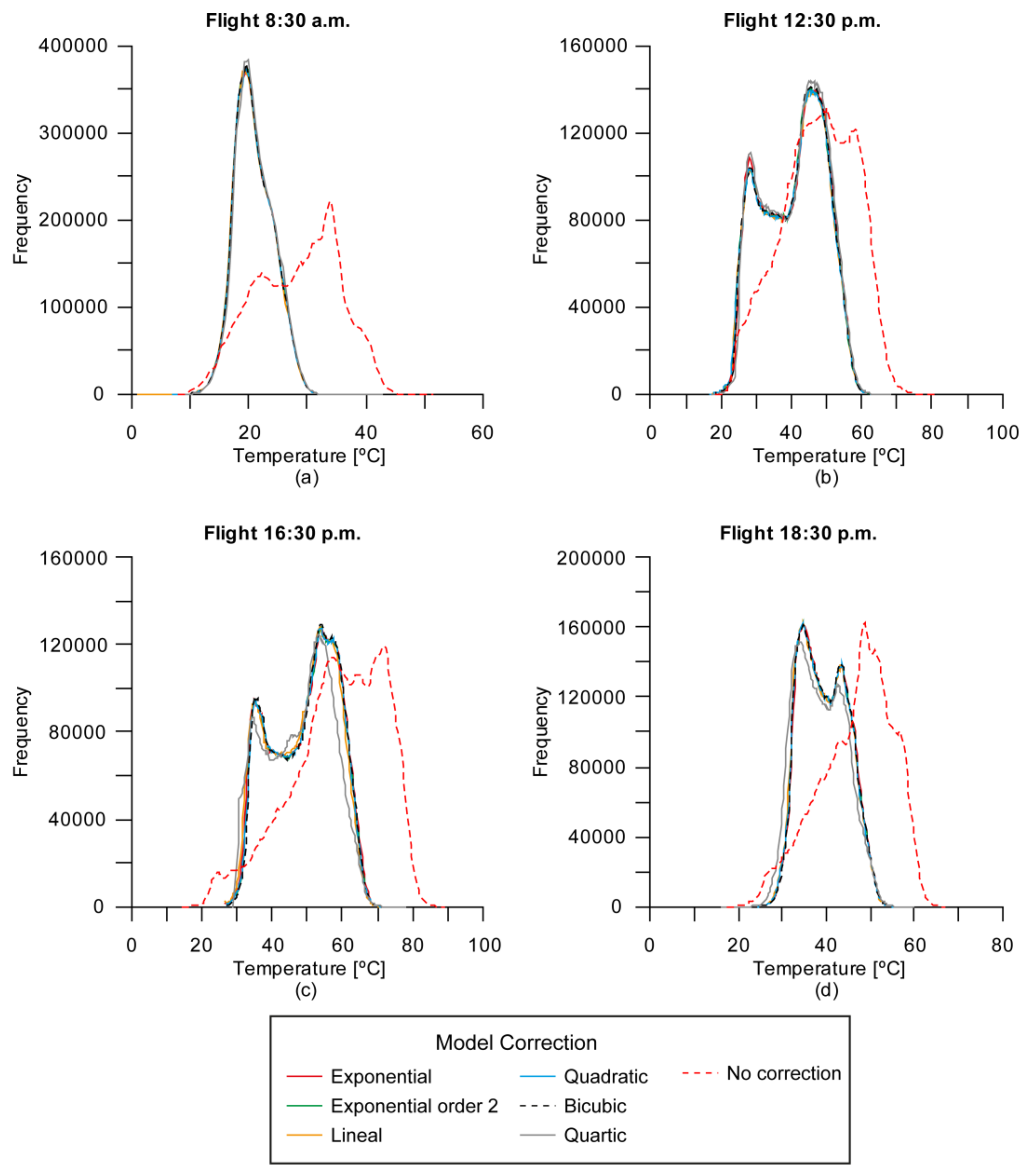
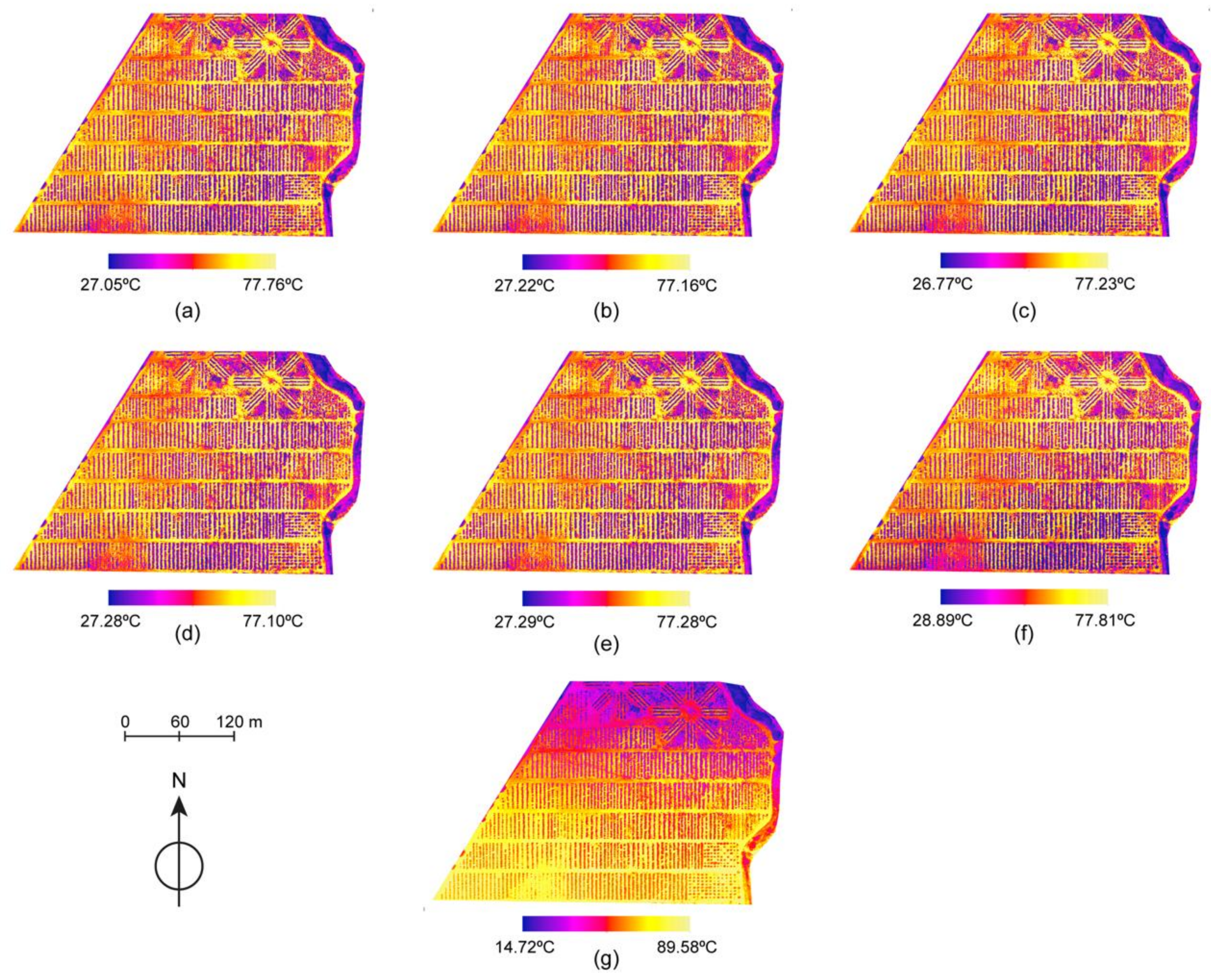
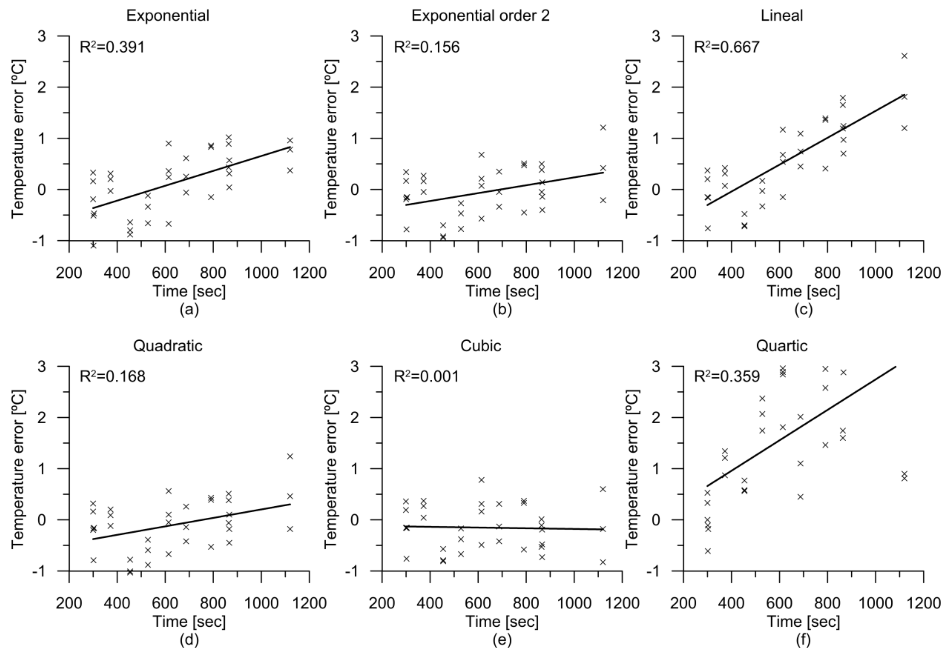
3. Results
Validation
4. Conclusions
Acknowledgments
Author Contributions
Conflicts of Interest
References
- Alexandratos, N.; Bruinsma, J. World Agriculture Towards 2030/2050: The 2012 Revision; Agriculture Development Economics Division Food and Agriculture Organization of the United Nations (FAO): Rome, Italy, 2012; Available online: http://www.fao.org/docrep/016/ap106e/ap106e.pdf (accessed on 16 April 2018).
- McCalla, A.F. Challenges to world agriculture in the 21st century. UPDATE Agric. Resour. Econ. 2001, 4. Available online: https://giannini.ucop.edu/publications/are-update/issues/2001/4/3/challenges-to-world-agric/ (accessed on 16 April 2018).
- Stafford, J.V. Implementing precision agriculture in the 21st century. J. Agric. Eng. Res. 2000, 76, 267–275. [Google Scholar] [CrossRef]
- Miao, Y.; Mulla, D.J.; Randall, G.W.; Vetsch, J.A.; Vintila, R. Combining chlorophyll meter readings and high spatial resolution remote sensing images for in-season site-specific nitrogen management of corn. Precis. Agric. 2009, 10, 45–62. [Google Scholar] [CrossRef]
- Mulla, D.J. Twenty five years of remote sensing in precision agriculture: Key advances and remaining knowledge gaps. Biosyst. Eng. 2013, 114, 358–371. [Google Scholar] [CrossRef]
- Goetz, A.F.H. Three decades of hyperspectral remote sensing of the earth: A personal view. Remote Sens. Environ. 2009, 113, S5–S16. [Google Scholar] [CrossRef]
- Anderson, K.; Gaston, K.J. Lightweight unmanned aerial vehicles will revolutionize spatial ecology. Front. Ecol. Environ. 2013, 11, 138–146. [Google Scholar] [CrossRef]
- Berni, J.A.J.; Zarco-Tejada, P.J.; Sepulcre-Cantó, G.; Fereres, E.; Villalobos, F. Mapping canopy conductance and cwsi in olive orchards using high resolution thermal remote sensing imagery. Remote Sens. Environ. 2009, 113, 2380–2388. [Google Scholar] [CrossRef]
- Colomina, I.; Molina, P. Unmanned aerial systems for photogrammetry and remote sensing: A review. ISPRS J. Photogramm. Remote Sens. 2014, 92, 79–97. [Google Scholar] [CrossRef]
- McBratney, A.; Whelan, B.; Ancev, T.; Bouma, J. Future directions of precision agriculture. Precis. Agric. 2005, 6, 7–23. [Google Scholar] [CrossRef]
- Lin, Y.; Hyyppa, J.; Jaakkola, A. Mini-uav-borne lidar for fine-scale mapping. IEEE Geosci. Remote Sens. Lett. 2011, 8, 426–430. [Google Scholar] [CrossRef]
- Wallace, L.; Lucieer, A.; Watson, C.; Turner, D. Development of a uav-lidar system with application to forest inventory. Remote Sens. 2012, 4, 1519–1543. [Google Scholar] [CrossRef]
- Torres-Sánchez, J.; Peña, J.M.; de Castro, A.I.; López-Granados, F. Multi-temporal mapping of the vegetation fraction in early-season wheat fields using images from uav. Comput. Electron. Agric. 2014, 103, 104–113. [Google Scholar] [CrossRef]
- López-Granados, F.; Torres-Sánchez, J.; Serrano-Pérez, A.; de Castro, A.I.; Mesas-Carrascosa, F.-J.; Peña, J.-M. Early season weed mapping in sunflower using uav technology: Variability of herbicide treatment maps against weed thresholds. Precis. Agric. 2016, 17, 183–199. [Google Scholar] [CrossRef]
- Mesas-Carrascosa, F.-J.; Torres-Sánchez, J.; Clavero-Rumbao, I.; García-Ferrer, A.; Peña, J.-M.; Borra-Serrano, I.; López-Granados, F. Assessing optimal flight parameters for generating accurate multispectral orthomosaicks by uav to support site-specific crop management. Remote Sens. 2015, 7, 12793–12814. [Google Scholar] [CrossRef]
- Candiago, S.; Remondino, F.; De Giglio, M.; Dubbini, M.; Gattelli, M. Evaluating multispectral images and vegetation indices for precision farming applications from uav images. Remote Sens. 2015, 7, 4026–4047. [Google Scholar] [CrossRef]
- Zarco-Tejada, P.J.; Guillén-Climent, M.L.; Hernández-Clemente, R.; Catalina, A.; González, M.R.; Martín, P. Estimating leaf carotenoid content in vineyards using high resolution hyperspectral imagery acquired from an unmanned aerial vehicle (uav). Agric. Forest Meteorol. 2013, 171–172, 281–294. [Google Scholar] [CrossRef]
- Hruska, R.; Mitchell, J.; Anderson, M.; Glenn, N.F. Radiometric and geometric analysis of hyperspectral imagery acquired from an unmanned aerial vehicle. Remote Sens. 2012, 4, 2736–2752. [Google Scholar] [CrossRef]
- Baluja, J.; Diago, M.P.; Balda, P.; Zorer, R.; Meggio, F.; Morales, F.; Tardaguila, J. Assessment of vineyard water status variability by thermal and multispectral imagery using an unmanned aerial vehicle (uav). Irrig. Sci. 2012, 30, 511–522. [Google Scholar] [CrossRef]
- Gonzalez-Dugo, V.; Zarco-Tejada, P.; Nicolás, E.; Nortes, P.A.; Alarcón, J.J.; Intrigliolo, D.S.; Fereres, E. Using high resolution uav thermal imagery to assess the variability in the water status of five fruit tree species within a commercial orchard. Precis. Agric. 2013, 14, 660–678. [Google Scholar] [CrossRef]
- Fereres, E.; Soriano, M.A. Deficit irrigation for reducing agricultural water use. J. Exp. Bot. 2007, 58, 147–159. [Google Scholar] [CrossRef] [PubMed]
- Calderón, R.; Navas-Cortés, J.A.; Lucena, C.; Zarco-Tejada, P.J. High-resolution airborne hyperspectral and thermal imagery for early detection of verticillium wilt of olive using fluorescence, temperature and narrow-band spectral indices. Remote Sens. Environ. 2013, 139, 231–245. [Google Scholar] [CrossRef]
- Zarco-Tejada, P.J.; González-Dugo, V.; Berni, J.A.J. Fluorescence, temperature and narrow-band indices acquired from a uav platform for water stress detection using a micro-hyperspectral imager and a thermal camera. Remote Sens. Environ. 2012, 117, 322–337. [Google Scholar] [CrossRef]
- Gonzalez-Dugo, V.; Hernandez, P.; Solis, I.; Zarco-Tejada, P.J. Using high-resolution hyperspectral and thermal airborne imagery to assess physiological condition in the context of wheat phenotyping. Remote Sens. 2015, 7, 13586–13605. [Google Scholar] [CrossRef]
- Chapman, S.C.; Merz, T.; Chan, A.; Jackway, P.; Hrabar, S.; Dreccer, M.F.; Holland, E.; Zheng, B.; Ling, T.J.; Jimenez-Berni, J. Pheno-copter: A low-altitude, autonomous remote-sensing robotic helicopter for high-throughput field-based phenotyping. Agronomy 2014, 4, 279–301. [Google Scholar] [CrossRef]
- Gallo, M.A.; Willits, D.S.; Lubke, R.A.; Thiede, E.C. Low-cost uncooled ir sensor for battlefield surveillance. Proceed. SPIE 1993, 2020, 351–362. [Google Scholar]
- Krupiński, M.; Bareła, J.; Firmanty, K.; Kastek, M. Test stand for non-uniformity correction of microbolometer focal plane arrays used in thermal cameras. Proc. SPIE Int. Soc. Opt. Eng. 2013, 8896. [Google Scholar] [CrossRef]
- Huawei, W.; Caiwen, M.; Jianzhong, C.; Haifeng, Z. An adaptive two-point non-uniformity correction algorithm based on shutter and its implementation. In Proceedings of the 2013 Fifth International Conference on Measuring Technology and Mechatronics Automation, Hong Kong, China, 16–17 January 2013; pp. 174–177. [Google Scholar]
- Olbrycht, R.; Więcek, B. New approach to thermal drift correction in microbolometer thermal cameras. Quant. InfraRed Thermogr. J. 2015, 12, 184–195. [Google Scholar] [CrossRef]
- Mudau, A.E.; Willers, C.J.; Griffith, D.; Roux, F.P.J.L. Non-uniformity correction and bad pixel replacement on lwir and mwir images. In Proceedings of the 2011 Saudi International Electronics, Communications and Photonics Conference (SIECPC), Riyadh, Saudi Arabia, 24–26 April 2011; pp. 1–5. [Google Scholar]
- King, S.R.; Rekow, M.N.; Carlson, P.S.; Heinke, T.; Warnke, S.H.; Brest, B. Shutterless Infrared Imager Algorithm with Drift Correction. Google Patents US8067735B2, 29 November 2011. [Google Scholar]
- Tempelhahn, A.; Budzier, H.; Krause, V.; Gerlach, G. Shutter-less calibration of uncooled infrared cameras. J. Sens. Sensor Syst. 2016, 5. [Google Scholar] [CrossRef]
- Mizrahi, U.; Fraenkel, A.; Kopolovich, Z.; Adin, A.; Bikov, L. Method and System for Measuring and Compensating for the Case Temperature Variations in a Bolometer Based System. US Patent No. US 7807968 B2, 5 October 2010. [Google Scholar]
- Harris, J.G.; Yu-Ming, C. Nonuniformity correction of infrared image sequences using the constant-statistics constraint. IEEE Trans. Image Process. 1999, 8, 1148–1151. [Google Scholar] [CrossRef] [PubMed]
- Zuo, C.; Chen, Q.; Gu, G.; Sui, X.; Ren, J. Improved interframe registration based nonuniformity correction for focal plane arrays. Infrared Phys. Technol. 2012, 55, 263–269. [Google Scholar] [CrossRef]
- Berni, J.A.J.; Zarco-Tejada, P.J.; Suarez, L.; Fereres, E. Thermal and narrowband multispectral remote sensing for vegetation monitoring from an unmanned aerial vehicle. IEEE Trans. Geosci. Remote Sens. 2009, 47, 722–738. [Google Scholar] [CrossRef] [Green Version]
- Zalameda, J.N.; Winfree, W.P. Investigation of uncooled microbolometer focal plane array infrared camera for quantitative thermography. J. Nondestruct. Eval. 2005, 24, 1–9. [Google Scholar] [CrossRef]
- Gómez-Candón, D.; Virlet, N.; Labbé, S.; Jolivot, A.; Regnard, J.-L. Field phenotyping of water stress at tree scale by uav-sensed imagery: New insights for thermal acquisition and calibration. Precis. Agric. 2016, 17, 786–800. [Google Scholar] [CrossRef]
- Jensen, A.M.; McKee, M.; Chen, Y. Procedures for processing thermal images using low-cost microbolometer cameras for small unmanned aerial systems. In Proceedings of the 2014 IEEE Geoscience and Remote Sensing Symposium, Quebec City, QC, Canada, 13–18 July 2014; pp. 2629–2632. [Google Scholar]
- Lowe, D.G. Distinctive image features from scale-invariant keypoints. Int. J. Comput. Vis. 2004, 60, 91–110. [Google Scholar] [CrossRef]
- Zarco-Tejada, P.J.; Berni, J.A.J.; Suárez, L.; Sepulcre-Cantó, G.; Morales, F.; Miller, J.R. Imaging chlorophyll fluorescence with an airborne narrow-band multispectral camera for vegetation stress detection. Remote Sens. Environ. 2009, 113, 1262–1275. [Google Scholar] [CrossRef]
- Torres-Rua, A. Vicarious calibration of suas microbolometer temperature imagery for estimation of radiometric land surface temperature. Sensors 2017, 17, 1499. [Google Scholar] [CrossRef] [PubMed]
- Honkavaara, E.; Saari, H.; Kaivosoja, J.; Pölönen, I.; Hakala, T.; Litkey, P.; Mäkynen, J.; Pesonen, L. Processing and assessment of spectrometric, stereoscopic imagery collected using a lightweight uav spectral camera for precision agriculture. Remote Sens. 2013, 5, 5006–5039. [Google Scholar] [CrossRef] [Green Version]
- Bellvert, J.; Zarco-Tejada, P.J.; Girona, J.; Fereres, E. Mapping crop water stress index in a ‘pinot-noir’ vineyard: Comparing ground measurements with thermal remote sensing imagery from an unmanned aerial vehicle. Precis. Agric. 2014, 15, 361–376. [Google Scholar] [CrossRef]
- Akaike, H. A new look at the statistical model identification. IEEE Trans. Autom. Control 1974, 19, 716–723. [Google Scholar] [CrossRef]


| UAV Flight (Local Time) | ||||
|---|---|---|---|---|
| 8:30 | 12:30 | 16:00 | 18:30 | |
| Air temperature (°C) | 21 | 30 | 36 | 37 |
| Relative humidity (%) | 48 | 26 | 18 | 17 |
| Mean wind speed (m/s) | 2 | 3 | 6 | 6 |
| Atmospheric pressure (hPa) | 1022.6 | 1021.2 | 1018.4 | 1017.4 |
| DCM Type | Time of Flight | Equation | |
|---|---|---|---|
| Exponential order 1 | 8:30 | 0.375 * | |
| 12:00 | 0.190 n.s. | ||
| 16:00 | 0.733 ** | ||
| 18:30 | 0.688 ** | ||
| Exponential order 2 | 8:30 | 0.382 * | |
| 12:00 | 0.398 * | ||
| 16:00 | 0.688 ** | ||
| 18:30 | 0.675 ** | ||
| Lineal | 8:30 | 0.370 * | |
| 12:00 | 0.210 n.s. | ||
| 16:00 | 0.688 ** | ||
| 18:30 | 0.673 ** | ||
| Quadratic | 8:30 | 0.379 * | |
| 12:00 | 0.286 n.s. | ||
| 16:00 | 0.755 ** | ||
| 18:30 | 0.676 ** | ||
| Bicubic | 8:30 | 0.380 * | |
| 12:00 | 0.482 * | ||
| 16:00 | 0.836 ** | ||
| 18:30 | 0.694 ** | ||
| Quartic | 8:30 | 0.381 * | |
| 12:00 | 0.474 * | ||
| 16:00 | 0.799 ** | ||
| 18:30 | 0.688 ** |
| Time of Flight | Exponential | Exponential Order 2 | Lineal | Quadratic | Cubic | Quartic | No DCM | |
|---|---|---|---|---|---|---|---|---|
| 8:30 a.m. | Range | 35.33 | 35.66 | 35.66 | 35.68 | 34.64 | 34.33 | 43.16 |
| Mean | 20.92 | 20.96 | 20.88 | 20.95 | 20.96 | 21.10 | 28.35 | |
| SD | 3.29 | 3.28 | 3.30 | 3.29 | 3.28 | 3.26 | 7.14 | |
| SBC | 0.38 | 0.38 | 0.38 | 0.38 | 0.38 | 0.38 | 0.47 | |
| 12:30 p.m. | Range | 50.08 | 50.03 | 50.15 | 50.31 | 49.80 | 50.72 | 62.38 |
| Mean | 40.74 | 40.50 | 40.53 | 40.48 | 40.61 | 40.98 | 47.68 | |
| SD | 8.87 | 8.89 | 8.92 | 8.91 | 8.87 | 8.80 | 10.43 | |
| SBC | 0.66 | 0.66 | 0.66 | 0.66 | 0.66 | 0.67 | 0.45 | |
| 16:00 p.m. | Range | 50.89 | 49.82 | 50.52 | 50.08 | 50.18 | 48.71 | 74.52 |
| Mean | 49.19 | 49.20 | 48.66 | 49.22 | 49.37 | 47.84 | 58.66 | |
| SD | 9.41 | 9.24 | 9.35 | 9.25 | 9.19 | 9.73 | 13.06 | |
| SBC | 0.68 | 0.68 | 0.68 | 0.68 | 0.68 | 0.65 | 0.48 | |
| 18:30 p.m. | Range | 43.78 | 39.65 | 42.83 | 41.17 | 42.46 | 43.74 | 49.57 |
| Mean | 39.57 | 39.47 | 39.37 | 39.46 | 39.55 | 38.61 | 46.69 | |
| SD | 5.24 | 5.26 | 5.28 | 5.24 | 5.23 | 5.55 | 8.32 | |
| SBC | 0.67 | 0.67 | 0.66 | 0.67 | 0.67 | 0.66 | 0.48 |
| Exponential | Exponential 2 | Lineal | Quadratic | Cubic | Quartic | No DCM | ||
|---|---|---|---|---|---|---|---|---|
| 8:30 | Mean | 1.013 | 0.898 | 0.913 | 0.901 | 0.888 | 0.895 | −2.929 |
| SD | 0.818 | 0.804 | 0.815 | 0.800 | 0.803 | 0.758 | 2.792 | |
| AIC | 3.777 | 0.832 | 3.593 | 2.574 | 0.779 | 18.472 | -- | |
| r2 | 0.027 | 0.004 | 0.001 | 0.005 | 0.049 | 0.645 ** | 0.918 ** | |
| 12:30 | Mean | 0.288 | 0.291 | 0.225 | 0.222 | 0.105 | 0.212 | −3.555 |
| SD | 0.590 | 0.560 | 0.556 | 0.569 | 0.459 | 0.584 | 3.012 | |
| AIC | 39.833 | 27.437 | 36.364 | 31.673 | 26.671 | 56.955 | -- | |
| r2 | 0.007 | 0.025 | 0.052 | 0.08 | 0.006 | 0.322 ** | 0.959 ** | |
| 16:30 | Mean | 0.112 | -0.152 | 0.518 | -0.123 | -0.065 | 1.573 | −12.158 |
| SD | 0.588 | 0.493 | 0.795 | 0.508 | 0.450 | 1.224 | 7.363 | |
| AIC | 18.219 | 7.452 | 11.329 | 7.765 | 2.314 | 31.893 | -- | |
| r2 | 0.391 ** | 0.156 * | 0.667 ** | 0.168 * | 0.001 | 0.359 ** | 0.915 ** | |
| 18:30 | Mean | 0.379 | 0.409 | 0.524 | 0.404 | 0.265 | 1.557 | −9.544 |
| SD | 0.648 | 0.622 | 0.627 | 0.626 | 0.585 | 0.857 | 5.433 | |
| AIC | 12.992 | 6.888 | 13.871 | 9.006 | 2.568 | 29.432 | -- | |
| r2 | 0.001 | 0.009 | 0.032 | 0.005 | 0.022 | 0.568 ** | 0.880 ** |
© 2018 by the authors. Licensee MDPI, Basel, Switzerland. This article is an open access article distributed under the terms and conditions of the Creative Commons Attribution (CC BY) license (http://creativecommons.org/licenses/by/4.0/).
Share and Cite
Mesas-Carrascosa, F.-J.; Pérez-Porras, F.; Meroño de Larriva, J.E.; Mena Frau, C.; Agüera-Vega, F.; Carvajal-Ramírez, F.; Martínez-Carricondo, P.; García-Ferrer, A. Drift Correction of Lightweight Microbolometer Thermal Sensors On-Board Unmanned Aerial Vehicles. Remote Sens. 2018, 10, 615. https://doi.org/10.3390/rs10040615
Mesas-Carrascosa F-J, Pérez-Porras F, Meroño de Larriva JE, Mena Frau C, Agüera-Vega F, Carvajal-Ramírez F, Martínez-Carricondo P, García-Ferrer A. Drift Correction of Lightweight Microbolometer Thermal Sensors On-Board Unmanned Aerial Vehicles. Remote Sensing. 2018; 10(4):615. https://doi.org/10.3390/rs10040615
Chicago/Turabian StyleMesas-Carrascosa, Francisco-Javier, Fernando Pérez-Porras, Jose Emilio Meroño de Larriva, Carlos Mena Frau, Francisco Agüera-Vega, Fernando Carvajal-Ramírez, Patricio Martínez-Carricondo, and Alfonso García-Ferrer. 2018. "Drift Correction of Lightweight Microbolometer Thermal Sensors On-Board Unmanned Aerial Vehicles" Remote Sensing 10, no. 4: 615. https://doi.org/10.3390/rs10040615