1. Introduction
Change detection in remote sensing is the process of detecting changes that have occurred on the Earth’s surface by remote-sensing images of the same region acquired at different times. In the past few decades, many change detection algorithms have been proposed and reviewed [
1,
2,
3,
4,
5], which can be simply divided into two categories of supervised and unsupervised.
Supervised change detection is to identify changes through the process of overlaying coincident thematic maps which are generated by classifying the images [
4]. The distinct advantage of this technique is that the change transitions are explicitly known. However, supervised change detection is limited by map production issues, and compounded by errors making it a costly and difficult method to adopt [
6].
This paper is focused on the unsupervised methods with two steps in a broad sense. The first is to produce a difference image to characterize the degree of changes. The second is to analyze the difference image to determine the final change detection result [
7,
8]. The difference image is usually produced by comparing the characteristics between two pixels by some unsupervised algorithms such as standard change vector analysis (CVA) [
9,
10], spectral angle mapper (SAM) [
11,
12], spectral correlation mapper (SCM) [
11], or spectral gradient difference (SGD) [
13]. Moreover, data transformations such as principle component analysis (PCA) [
14,
15,
16,
17], or multivariate alteration detection (MAD) [
18] can also generate the difference image by suppressing correlated information and highlighting variance. The second step, which can be seen as a binary classification or segmentation problem, labels the pixels in the difference image as the changed or unchanged class. The commonly used segmentation algorithms in the second step are the thresholding [
19,
20], the fuzzy set theory [
15], the expectation maximization algorithm (EM) [
21,
22], the Markov random fields (MRF) [
23,
24] and the conditional random field (CRF) [
25].
Producing the difference image is the key to the unsupervised change detection, and it should truly characterize the degree of the change of every pixel. Unsupervised methods usually require a priori assumption that is the basis for modeling ‘change’ [
14,
26]. Data transformations such as PCA and MAD assume that multi-temporal data is highly correlated and change information can be highlighted in the new components or MAD variates. PCA puts two dates of images into a single file; then performs principal component transformation and analyses the minor component images for change information [
2]. However, it is difficult to decide appropriate components especially for multispectral or hyperspectral remote-sensing images. MAD may become unstable when features are highly correlated [
18]. Moreover, MAD requires a large portion of the image is unchanged; otherwise the result will be inaccurate or even completely wrong.
The more widely used unsupervised change detection methods compare the characteristics of the pixels in two images directly. The CVA assumes that the degree of change is determined by the variation in spectral values which is computed by the distance between spectral vectors. Usually, the distance measure is the Euclidean distance, while the chi-square transformation method uses the Mahalanobis distance [
27]. An advantage of chi-square transformation is that it increases the importance of bands having little variation in reflectance [
11], in contrast to the standard CVA with the use of Euclidean distance. However, chi-square transformation requires a large portion of the scene is unchanged just like MAD, and the changes related to specific spectral direction may not be as readily identified [
27].
SAM, SCM and SGD model the variation in spectral shapes from different perspectives. SAM computes the cosine correlation [
11] between spectral vectors, while SCM computes the Pearson’s correlation [
28] between them. SAM can eliminate the effects of shade to a certain extent, which is important for change detection since illumination variation and shadow are unavoidable in multitemporal images. However, SAM is unable to detect negatively correlated data, and cosine correlation is sensitive to additive factors. SCM is the normalization form of SAM, and it is invariant to linear transformation of the data. That is, if two spectral curves are identical, but changed by a multiplicative factor or by an additive factor, the correlation remains 1. Therefore, SCM performs better than SAM in eliminating the effects of shadows and illumination variation.
SAM and SCM indirectly compute the difference in spectral shapes without representing the spectral shape of each spectral curve, while SGD directly represents the spectral shapes by spectral gradients [
29]. The degree of change is calculated by the difference of the spectral gradients between two spectral curves [
13]. It is not always appropriate to assume the cosine correlation or the Pearson’s correlation between spectral vectors can characterize the degree of change between them. Therefore, SGD has been proved to outperform other two methods in change detection [
13]. However, SGD is sensitive to gain factors in theory, that is, SGD cannot eliminate the effects of illumination variation and shadows. To get a better representation of the difference between spectral shapes, a new method which combines SGD and SCM is proposed.
In this paper, the method based on the variation in spectral values is referred to CDSV (change detection based on spectral values), and the method based on the variation in spectral shapes is referred to CDSS (change detection based on spectral shapes). It is difficult to identify correctly all change types using only CDSV or CDSS, because different change types have different spectral curves. For example, the change between two pixels will be easily missed by CDSV if both are dark. In other words, the credibility of CDSV is low for this change type. Besides, the change tends to be missed by CDSS if two pixels have “close-to-flat” spectral curves (which means the spectral curves are close to flat). In other words, the credibility of CDSS is low for this change type.
According to the above analysis, this paper presents a new hybrid spectral difference (HSD) method, considering the difference of both spectral values and spectral shapes. Firstly, two difference images are produced by CDSV and CDSS, respectively. Then, the credibility of two methods is calculated. Finally, two difference images are fused with the corresponding credibility to produce the result.
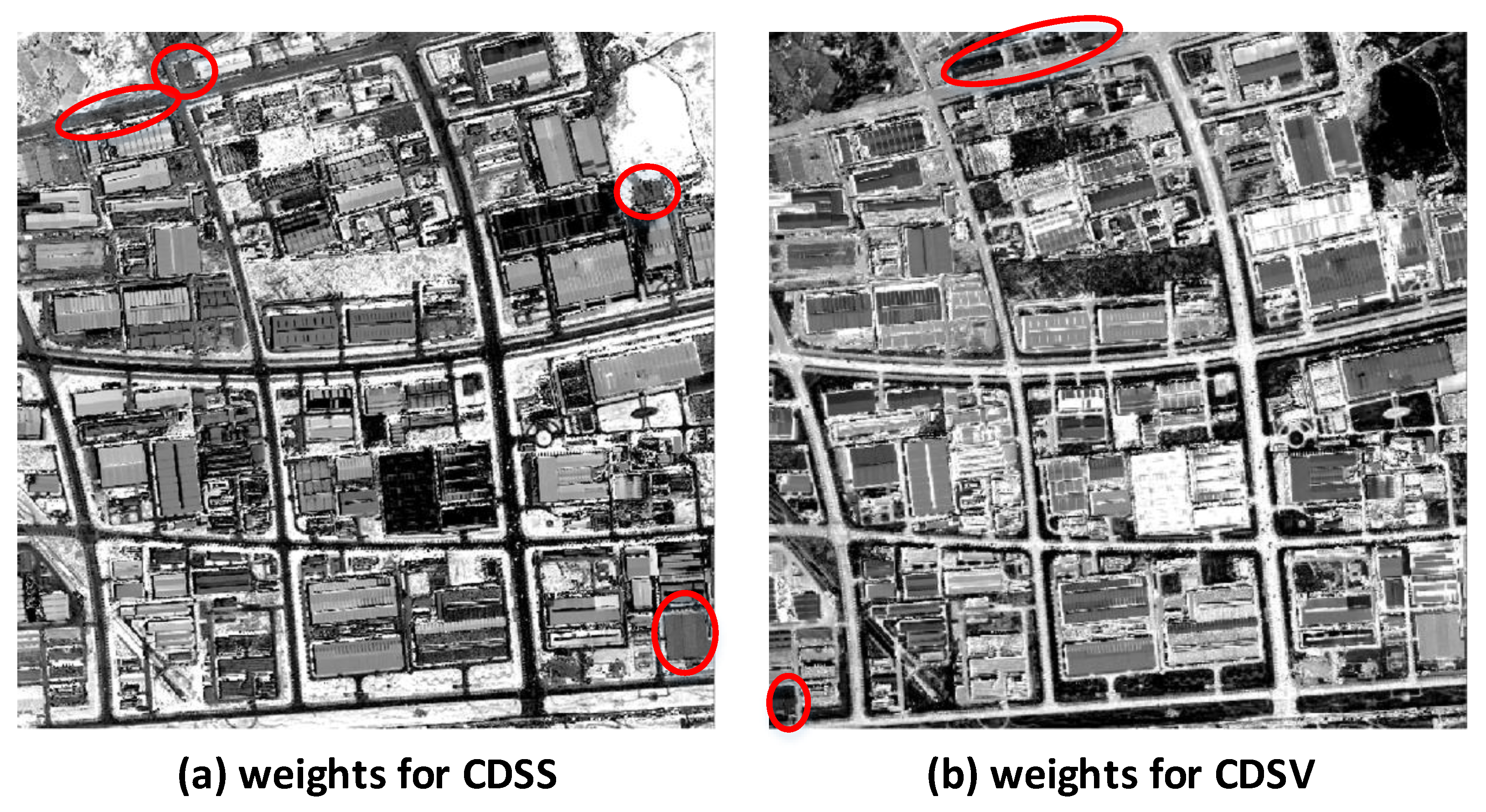
The superiority of HSD lies in the calculation of weights in the fusion of CDSS and CDSV. The weights are calculated by the credibility of two methods. For example, if CDSS has high credibility and CDSV has low credibility for a changed pixel, CDSV tend to miss the change but have the low weight in the fusion, and CDSS tend to find the change and have the high weight in the fusion. Therefore, HSD will find the change which is missed by only one method.
The rest of this paper is organized as follows. The next section presents the theory of the proposed method.
Section 3 presents the results of two experiments on different datasets.
Section 4 presents the discussion. The conclusions are presented in
Section 5.
2. Methodology
Let , represent two co-registered remote-sensing images with bands. There are three major steps for HSD to obtain the difference image: (1) generate two difference images by CDSV and CDSS; (2) calculate the credibility of the two methods; (3) fuse two difference images with the corresponding credibility.
2.1. Preprocessing
During data preprocessing, atmospheric correction [
30,
31], geometric and relative radiometric corrections would be carried out to make the two images as comparable as possible. Atmospheric correction and geometric correlation would be implemented by Envi5.3 and ERDAS IMAGINE 2014 respectively.
In the present work, relative radiometric normalization was implemented based on pseudo-invariant features (PIFs) [
32,
33] with an assumption that the invariant pixels in both images are linearly related, and PIFs are unchanged pixels only affected by radiometric variance [
34].
The selection of PIFs would be decided by CDSV, SCM and SGD together. We assume that at least
of the scene is unchanged, which is right in most applications. Three difference images are produced by three algorithms respectively. Then, the ‘unchange map’ of each algorithm is produced by thresholding the corresponding difference image and the darker
of the image is labeled as unchange. Let
,
,
represent the ‘unchange map’ of CDSV, SGD and SCM respectively, and PIFs can be selected by the following equation:
The main purpose of this framework is to compare and assess the algorithms fairly, as the relative radiometric normalization has a big influence on change detection. HSD was a fusion of CDSS and CDSV, and CDSS was a fusion of SGD and SCM. The PIFs are decided by the areas identified as unchanged by CDSV, SCM and SGD together, so the relative radiometric normalization will not influence the comparison of these algorithms.
2.2. Change Detection Based on Spectral Value (CDSV) and Change Detection Based on Spectral Shapes (CDSS) Algorithms
This section details with the CDSV and CDSS for producing two difference images by spectral values and shapes respectively.
2.2.1. CDSV Algorithm
The Euclidean distance between spectral vectors can characterize the difference between spectral values excellently. Although the Mahalanobis distance can increase the importance of bands having little variation of reflectance, image normalization already ensures that each band has the same impact on change detection. Let
represent the difference image produced by CDSV [
9,
10]:
where
and
repersents the
i-th band in
and
respectively.
2.2.2. CDSS Algorithm
SCM and SGD represent the difference in spectral shapes from different perspectives. SCM computes the difference between spectral shapes by the Pearson’s correlation of them. Let
be the difference image obtained by SCM [
11,
28]:
where
and
represent the mean of all the bands of
and
, L represents the number of bands and the superscript
means the i-th band. SCM computes the Pearson’s correlation between spectral vectors, so the value range is [−1, 1].
SGD directly represents the spectral shape by the spectral gradient. Let
represent the spectral gradient and
be the difference image produced by SGD [
13,
29]
where the superscript
and subscript
means the
i-th band in the
k-th image, L represents the number of bands.
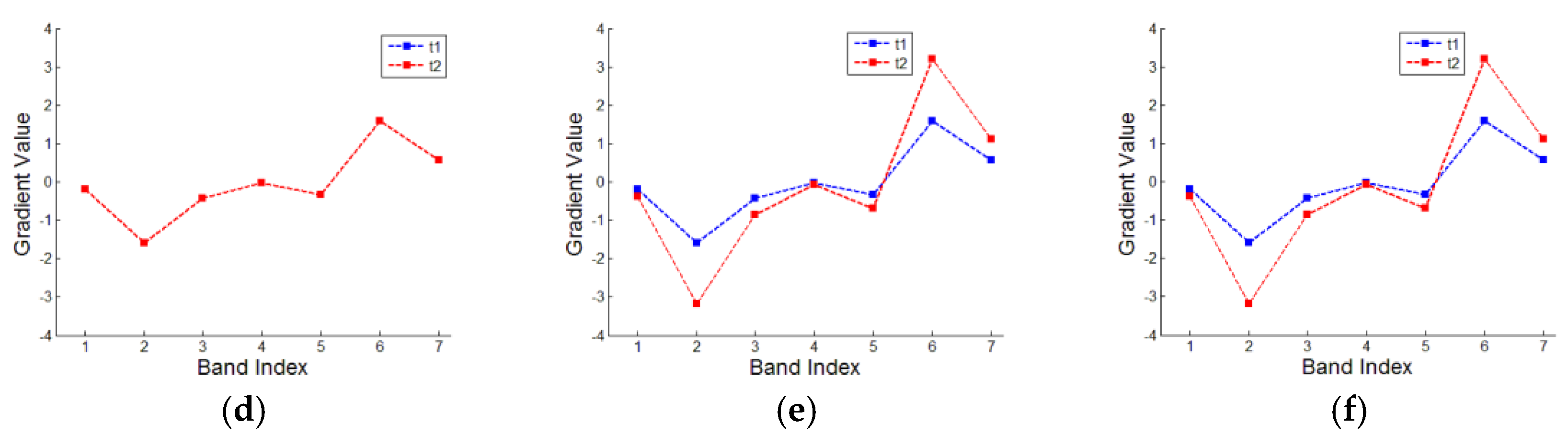
In
Figure 1, the blue curve is a spectral curve or the corresponding spectral gradients of a pixel in WordlView-2 image, and the red curve is the simulation of pseudo changes. The simulated spectra are changed by an additive factor of 1 in
Figure 1a, a multiplicative factor of 2 in
Figure 1b, and both two factors in
Figure 1c. The spectral gradient curves are just below the corresponding spectral curves. We can find that two gradient curves coincide in
Figure 1d, and the gradient curves in
Figure 1e,f are identical. Therefore, SGD is insensitive to the additive factor even if the spectra are changed by a multiplicative factor simultaneously. However, the multiplicative factor is of negative impact on SGD, because the two gradient curves in
Figure 1e are different from each other.
In practice, the spectral changes caused by multiplicative and additive factors cannot be avoided because of shading, illumination variation, clouds and sensor calibration. The Pearson’s correlations between two curves in
Figure 1a–c are all 1, because SCM is insensitive to linear transformation of the spectra. SCM has an imperfect assumption that Pearson’s correlation between spectral vectors is negatively correlated with the degree of change between them, which is not always true in practice, because the correlation between spectra of different objects is arbitrary. For example, the degree of change of negatively correlated spectral vectors cannot be regarded as higher than it of uncorrelated ones. What can be sure is that spectral vectors of changed areas are not highly positively corrected, but there is no specific mathematic relationship between Pearson’s correlation and the degree of change.
Consequently, this paper proposes a new method which combines SCM and SGD to comprehensively consider the variation in spectral shapes, and the method is referred to CDSS. Let
represents the difference image produced by CDSS:
CDSS can be seen as a weighted SGD method, and the weight is decided by Pearson’s correlation between spectral vectors. When spectral changes are caused by multiplicative factors, SGD might wrongly identify it as change, so the weight for SGD needs to be low. The weight is negatively correlated with Pearson’s correlation, so it is decided by and is normalized by being divided by 2 as the righthand part in Equation (6). When the Pearson’s correlation between two curves is close to 1, the value of will be close to 0 even if the value of is high, so CDSS is insensitive to multiplicative factors and can eliminate the pseudo changes caused by illumination variation and shadow.
2.3. The Credibility of CDSV and CDSS
Since the credibility of CDSV is low when the pixels at different times are dark, we can calculate the spectral magnitude of each pixel at both times and use the larger one to represent the credibility. Let
representthe credibility of CDSV:
where
represent the spectral magnitude of the
k-th image.
The key to describing the credibility of CDSS is to quantify how steep the spectral curves are. This paper uses spectral gradient to describe the spectral shape, and the magnitude of spectral gradient can be an indicator to describe how steep the curve is. Therefore, we can calculate the magnitude of the spectral gradients of each pixel at both times and use the larger one to represent the credibility. Let
representthe magnitude of the spectral gradient of the
k-th image, and
represent the credibility of CDSS:
2.4. The Hybrid Spectral Difference (HSD) Algorithm
The HSD algorithm fuses DISV and DISS with their corresponding credibility. Let
be the difference image produced by HSD, and we can get
as follows:
where
and
represent the weights in the fusion process. To ensure that every pixel in
and
satisfies
, the weights can be calculated by the credibility as follows:
However, it is not appropriate to calculate and by and directly, because and have different pixel value range and distributions. Usually, pixels in have much higher values than pixels in ; therefore, most pixels in would have higher values than them in . As a result, would play a predominant role in the fusion process.
To ensure that the weights can correctly describe the importance of and , and should have the same pixel value distributions, that is, their histograms should be the same. There are two ways to ensure that two images have the same pixel value distributions:
Before histogram processing, the linear stretching needs to be applied to the images to ensure that the range of pixel values is 0 to 255. It is better to adopt histogram equalization rather than histogram matching to make and have the same histograms, because histogram equalization makes pixel values distributed evenly from 0 to 255. The histogram matching may lead to a narrow range of pixel values, which may cause the most pixel values in and to be close to 0.5, so the weights lose their effectiveness.
Let
and
be the
and
after histogram equalization; then Equations (12) and (13) are changed to:
Similarly,
and
should have the same histograms before fusion by Equation (11). Just like
and
, linear stretching should be applied to
and
before histogram processing, but here the histogram matching transformation is adopted rather than histogram equalization. Normally, only a small portion of the scene is changed in most applications, so DISV and DISS are dominated by large, dark areas, resulting in histograms characterized by a large concentration of pixels having levels near 0. In this circumstance, the histograms cannot become uniform by histogram equalization transformation, and a very narrow interval of dark pixels is mapped into the upper end of the gray levels of the output images [
35]. What’s more, the histogram equalization will compress the gray levels which are occupied by very little pixels and the output image would have few intensity levels occupied, hence, some changed area may be merged into unchanged area.
Let
and
be
and
after linear stretching, and chooses
as the specified image. Let
be
after histogram matching transformation, Equation (11) is changed to:
with
and
are calculated by Equations (14) and (15). And the flowchart of the HSD is shown in
Figure 2.
2.5. Accuracy Assessment and Reference Map
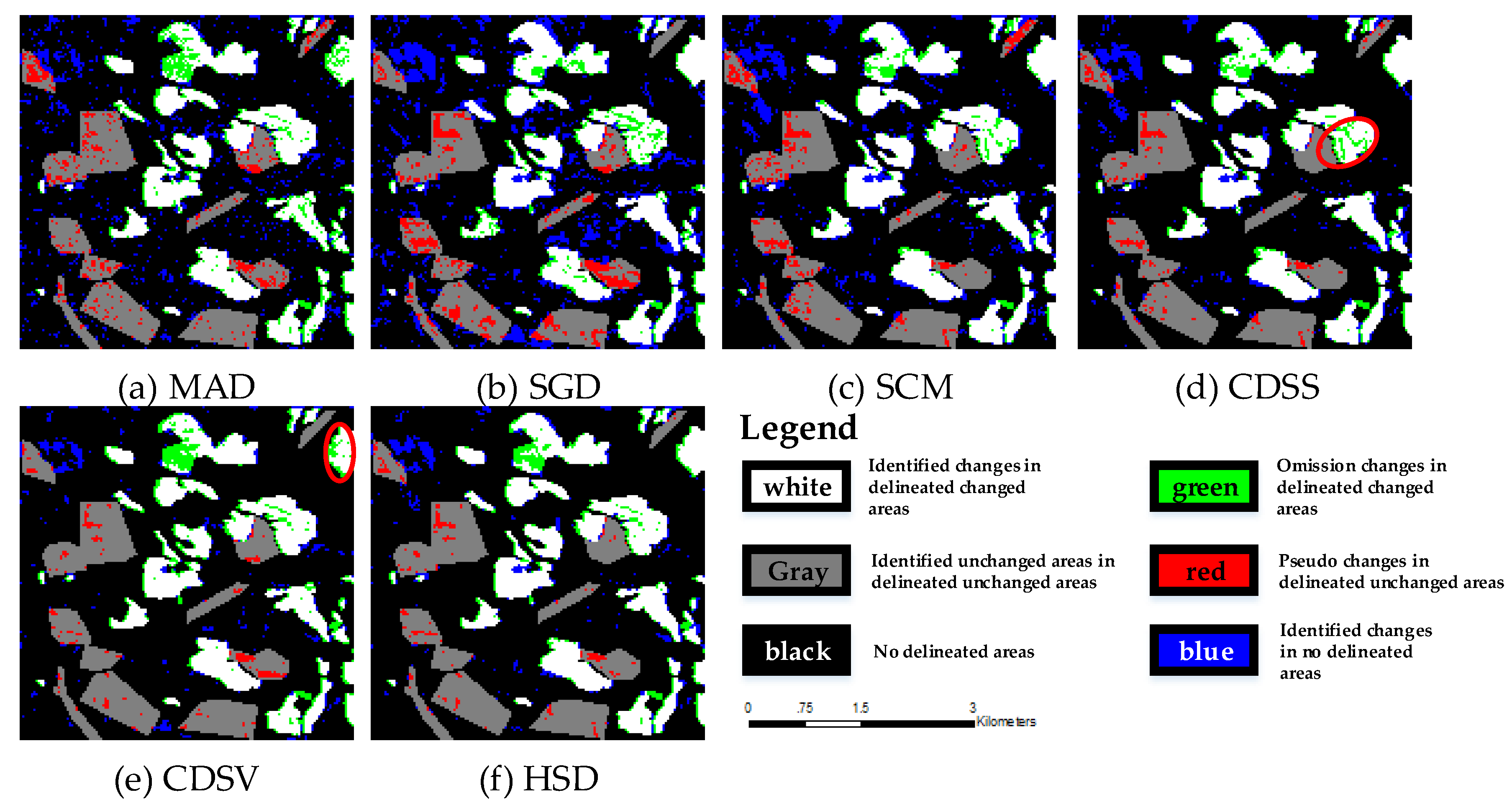
To prove the validity and effectiveness of the proposed algorithm, HSD, three algorithms which are used to generate HSD and other two algorithms were implemented for comparison. Each algorithm generated a difference image, but the result needed an appropriate threshold. The threshold directly affected the accuracy of the change detection. A series of thresholds were set by adjusting the parameters, and the calculation method was as follows:
where
and
represent the mean and standard deviation of the difference image.
was a series of adjustable parameters with equidistant intervals and the range of
varied in different experiments.
After binarizing the difference images, the results would be evaluated by the reference image using the omission rate and the commission rate which are widely used in change detection assessment [
5]. The omission rate is used to show the algorithm’s ability to find real changes while the commission rate is used to show the algorithm’s ability to avoid producing pseudo changes. Let
represent the number of changed pixels in the reference image,
represent the number of changed pixels correctly identified, and
represent the number of pixels of pseudo changes. Then, the omission rate and commission rate are calculated as follows:
The reference map made from manual interpretation was important for accuracy assessment. Normally, change maps were constructed with three areas of changed, unchanged and undefined. Foody found that the percentage of change would impact the accuracy assessment and approximately 50% of change would make both of sensitivity and specificity reach balance [
36,
37,
38]. In this paper, change maps would contain approximately equal area of changed and unchanged areas to allow algorithms to be evaluated and compared better.
Apart from the omission rate and the commission rate, the kappa coefficient [
39] is also used to assess algorithms. Some researches showed that kappa indices had flaws [
40,
41] and other advanced assessment features performed better such as quantity disagreement, allocation disagreement [
40] or Bradley–Terry model [
41]. Still, the kappa coefficient is widely used and acceptable in change detection assessment, as change detection can be seen as a simple classification problem with only two categories.
5. Conclusions
This paper proposes a novel approach to unsupervised change detection based on hybrid spectral difference (HSD). The main idea of HSD is to combine the two types of spectral differences: (a) spectral shapes; (b) spectral values. First, this paper uses a new method referred to CDSS which fuses the difference images produced by SCM and SGD to describe the variation in spectral shapes. Second, CDSV, which computes the Euclidean distance between two spectral vectors, is used to obtain a difference image based on the variation in spectral values. Then, the credibility of two types of spectral characteristics for every pixel is calculated to describe how appropriate these two spectral characteristics are for detecting the change. Finally, the difference images produced by CDSS and CDSV are fused with the corresponding credibility to generate the hybrid spectral difference image.
Two experiments were carried out to confirm the effectiveness of HSD. Both qualitative and quantitative results indicate that HSD had superior capabilities of change detection compared with CDSS, CDSV, SCM, SGD and MAD. The accuracy of CDSS is higher than CDSV in case-1 but lower in case-2, and compared to the higher one, the overall accuracy and the kappa coefficient of HSD improved by and and the omission rate dropped by in the first experiments; the overall accuracy and the kappa coefficient of HSD improved by and and the omission rate dropped by in the second experiments.
CDSS tends to miss the real changes if both spectral curves are close to flat, and CDSV tends to miss the changes if both pixels are dark. HSD used the credibility to compute the weights in the fusion, and successfully detected more changes.
The advantages of the method proposed in this paper are two-fold. First, HSD is highly automatic, and the only parameter in HSD is the threshold of the difference image. Second, HSD successfully combines the advantage of CDSS and CDSV and can detect more changes.
However, some change types are difficult to detect by only the spectral features of individual pixels. To solve this problem, texture features like grey-level co-occurrence matrix (GLCM) [
46] and histogram of oriented gradients (HOG) [
47], which use context information, can be used in our future investigations.


