An Exploration of Terrain Effects on Land Surface Phenology across the Qinghai–Tibet Plateau Using Landsat ETM+ and OLI Data

Abstract

Detecting spatial patterns of land surface phenology (LSP) with high spatial and temporal resolutions is crucial for accurately estimating phenological response and feedback to climate change and biogeochemical cycles. Numerous studies have revealed LSP across the Qinghai–Tibet Plateau (QTP) using a variety of coarse-resolution satellite data. However, detailed phenological spatial patterns along with changes of mountain topography remain poorly understood, which greatly limits efforts to predict the impacts of climate change on vegetation growth and ecosystem productivity in complex terrain regions. Combining Landsat 7 ETM+ (Enhanced Thematic Mapper Plus) and Landsat 8 OLI (Operational Land Imager) observations in overlapping zones of adjacent images, this study detected Normalized Difference Vegetation Index (NDVI)-based LSP metrics at a spatial resolution of 30 m, and explored how LSP varied with topographic factors along a 2600 km belt transect of the central QTP. The results show that the greenup onset date showed a delayed tendency with the increase of elevation at a mean rate of 1.52 days/100 m, while the dormancy onset date indicated an advanced tendency at a mean rate of −0.59 days/100 m. In general, greenup onset date was later but dormancy onset date was earlier on shaded slopes than on sunlit slopes in the meadow area. By contrast, greenup onset date did not significantly depend on aspect in the steppe area, while dormancy onset date indicated a similar response to aspect in the steppe area with that in the meadow area. With regard to the effect of slope on vegetation phenology in the meadow area, greenup onset date was significantly delayed but dormancy onset date significantly advanced with the increase of slope on both north and south slopes. In the steppe area, however, the influence pattern of slope on vegetation phenology was the opposite. Essentially, effects of topographical parameters on LSP were controlled by temperature and moisture combinations in complex terrain.

1. Introduction

Phenology is the study of recurring plant and animal life cycle stages, especially their timing and relationships with weather and climate [1]. Plant phenology focuses on the timing of annually recurring plant growth and reproductive phenomena, as well as the drivers of these events associated with endogenous and exogenous forces [2]. Plant phenological variation is highly sensitive to climate change and has strong feedbacks to the climate system [3]. Since the Qinghai–Tibet Plateau (QTP) has experienced a rapid warming that is twice as high as the global average level in recent decades [4], climate change and its impacts on alpine vegetation phenology have been the source of much concern [5,6,7,8,9]. To date, most land surface phenological studies on the QTP were based on Normalized Difference Vegetation Index (NDVI), Enhanced Vegetation Index (EVI), and Leaf Area Index (LAI) data from the Advanced Very High Resolution Radiometer (AVHRR) [5,6,10,11,12,13,14,15,16,17], Moderate-Resolution Imaging Spectroradiometer (MODIS) [6,7,8,14,18], and Satellite Pour l’Observation de la Terre (SPOT) [6,7,8,14,19,20,21]. The spatial resolutions of these data range normally from 500 m to 8 km. Thus, the extracted phenological metrics generally represent the composite of various vegetation types in a relatively large terrain unit and have been used to detect general phenological response to climate change at regional scales. By contrast, detailed spatial phenological patterns and their response to localized climatic factors remain poorly understood, which might lead to an inaccurate estimate of carbon budgets and ecosystem productivity on the QTP. To investigate spatial phenological responses to localized climatic factors, topographic features (such as slope, aspect, and elevation) at higher spatial resolution (such as 30 m) that control vegetation properties and growth conditions at local areas [22,23,24] can be used as a proxy for localized climatic factors. This is based on the fact that the spatial resolutions of gridded climate datasets currently available are normally coarser than 0.05 degrees [25], which is unable to represent the microclimate differentiation on the highly heterogeneous QTP.

Landsat sensors observe the land surface at a spatial resolution of 30 m with a repeat cycle of 16 days. However, Landsat observations with low cloud coverage are very limited within a year for most areas on the Earth [26]. Therefore, multiyear Landsat NDVI/EVI data have been combined to improve the temporal resolution for phenological detection [27,28,29]. This kind of phenological detection can capture multiyear mean vegetation dynamics at higher spatial resolution than that with satellite data from other sensors with more frequent repeat cycles. In addition, interannual variation of vegetation phenology could be derived by computing the annual anomaly in the timing (day of year) of the spring onset and autumn onset relative to the long-term average [29,30]. This approach can produce reasonable interannual phenological variation in North American temperate and boreal deciduous forests [28,29,31], and mixed and conifer-dominated forests [31]. Alternatively, the temporal resolution of Landsat data can also be improved by fusing Landsat streams with daily MODIS data for detailed analysis of vegetation phenology [32,33,34]. The basic assumption in current data fusion methods is that the vegetation growth rate is the same within a land cover type [35]. It should be noted that although these approaches may roughly retrieve multiyear mean and yearly land surface phenology from Landsat data, accurate vegetation phenology timing metrics should be derived from Landsat observations in the same year. Therefore, our research developed a new approach to estimate the grassland LSP using a single-year NDVI curve on the QTP.

The overall objectives of this study are to (1) extract vegetation phenology at each pixel along a transect across the middle of the QTP based on the Landsat observations in the same year; (2) quantify the impacts of topographic features on spatial heterogeneity of vegetation phenological metrics; and (3) explain the climatic cues of terrain effects. To achieve these goals, we combined Landsat 7 ETM+ (Enhanced Thematic Mapper Plus) and Landsat 8 OLI (Operational Land Imager) at the overlapping zones of adjacent images across the middle of the QTP from 2013 to 2015. This combination could provide as many as 92 observations within a year, which is potentially able to produce fairly accurate phenological timings [36].

2. Materials and Methods

2.1. Study Area and Vegetation Types

The Qinghai–Tibet Plateau is located in western and southwestern China, covering approximately 2.3 million km², which accounts for about a quarter of China’s land area. The elevation on the QTP increases rapidly from about 2000 m in the east to more than 8000 m in the west with an average elevation exceeding 4000 m. Influenced by both elevation and Indian monsoon, the climate shows a thermal/moisture gradient from southeast to northwest. According to the climate regionalization scheme [37], the climate of the QTP can be divided into plateau’s temperate humid region, plateau’s temperate and subalpine subhumid region, plateau’s temperate and subalpine semiarid region, and plateau’s temperate and alpine arid region. The annual mean air temperature decreases from 15.5 °C in the southeast to −5.0 °C in the northwest and the annual mean total precipitation decreases from 1764 mm in the southeast to 16 mm in the northwest for the period of 1981 to 2011 [9]. The dominant vegetation types along the thermal/moisture gradient include forest, shrub, meadow, steppe, and desert [38].

In this study, we focused on steppe and meadow (Figure 1). These two major vegetation types are distributed across the QTP except for southeastern forest/shrub areas and northwestern desert areas, and cover about 60% of the QTP. Specifically, meadow is mainly concentrated in the central, eastern, and southern areas with temperate and subalpine subhumid climate, while steppe appears mostly in the western and northern areas with temperate and subalpine semiarid and arid climate.

2.2. Satellite Data and Data Processing

A total of 4135 Landsat ETM+ (Enhanced Thematic Mapper Plus) and OLI (Operational Land Imager) images from 2013 to 2015 were obtained from the United States Geological Survey (USGS) archive (http://earthexplorer.usgs.gov/). Based on these data, 17 Landsat overlapping zones of adjacent images were selected along a transect across the middle of the QTP following the elevational gradient from east to west (Figure 1). Fewer OLI images are available in 2013 than in 2014 and 2015 because Landsat 8 launched in February 2013 (Figure A1 in Appendix A). To reduce atmospheric effects, raw digital number values from each image were converted to surface reflectance using the atmosphere correction tool in the Landsat Ecosystem Disturbance Adaptive Processing System (LEDAPS) [39,40]. Surface reflectance data from both Landsat 7 and 8 images were used to calculate the Normalized Difference Vegetation Index (NDVI). In addition, we used the Fmask product [41,42] to remove cloud, cloud shadow, snow cover, and open water.

NDVI from Landsat 7 ETM+ was calibrated to be comparable to that from Landsat 8 OLI. A uniform transformation function between OLI NDVI and ETM+ NDVI values was developed based on datasets in the United States, which was assumed to be applicable for various regions and time periods [43]. However, we found that the transformation function varied considerably on the QTP. Thus, we established a set of temporally local functions using linear regressions between spatial OLI and ETM+ NDVI data pairs in temporally adjacent time phases in each zone. The temporally local functions were applied to calibrate Landsat 7 ETM+ NDVI.

The MODIS land surface temperature (LST) product (MOD11A2) with a temporal resolution of 8 days and spatial resolution of 1000 m from 2013 to 2015 was also acquired from the USGS archive (http://earthexplorer.usgs.gov/), and was then used to determine the winter period based on a threshold of 278 K. The maximum NDVI during the winter was taken as the background value for vegetation dormancy because temporal NDVI variation below 278 K reflects snow contamination [44]. To match the spatial resolution of Landsat observations, LST data were resampled into 30 m resolution using a nearest neighbor method.

2.3. Land Surface Phenology Extraction Using Landsat Data

The Hybrid Piecewise Logistic Model (HPLM) algorithm [44], which was developed by combining a piecewise logistic model [45] with greenness under stress [29,46], has been used to detect phenological metrics from AVHRR, MODIS, and VIIRS (Visible Infrared Imaging Radiometer Suite) data [47,48]. A sensitive analysis indicated that vegetation phenology can be estimated precisely from satellite data with temporal resolutions of 6–16 days [36]. Therefore, we assumed that the HPLM algorithm is appropriate for phenology detection combining Landsat 7 and 8 “overlapping” regions where the temporal resolution could be as fine as 4 days. Land surface phenology in this study was extracted from ETM+ and OLI NDVI (Figure 2) using the HPLM algorithm. The HPLM divided a vegetation growing cycle into greenup phase and senescence phase using the slope within a moving window of five NDVI observations. In each phase, we fitted NDVI time series using HPLM:

$$NDVI\left(t\right)=\frac{c_1}{1+e^{a_1+b_{1}t}}+NDV{I}_b$$

(1)

$$NDVI\left(t\right)=\frac{c_2+dt}{1+e^{a_2+b_{2}t}}+NDV{I}_b$$

(2)

where $t$ is time in day of year (DOY); $a_1$ and $a_2$ are related to the vegetation growth time; $b_1$ and $b_2$ are associated with the rate of plant leaf development; $c_1$ and $c_2$ are the amplitude of the NDVI variation; $d$ is the vegetation stress factor; and $NDV{I}_b$ is the background NDVI value. Equation (1) represents the favorable growth condition and Equation (2) denotes vegetation growth suffering from stress. After comparing the fitting goodness of Equations (1) and (2), the better equation was chosen for extracting phenological timing metrics.

The phenological transition dates were then identified using the rate of curvature change on the NDVI curve modeled by HPLM [45]. Specifically, the timings corresponding to the extreme values in the rate of curvature change were considered as phenological dates, namely, greenup onset date (GO) and dormancy onset date (DO) (Figure 2).

2.4. Evaluation of Phenological Extraction

The confidence level of phenological extraction was measured by the proportion of good-quality observations during a vegetation growing cycle and the fitness of HPLM modeling of the NDVI time series [44]. The proportion of good-quality observations (PGQ) during the growing season was used to qualify if the phenology is appropriately detected. The PGQ can only be calculated after phenological date detections because phenological metrics could be well detected even if missing land surface observations occur during the vegetation dormancy period. In general, high PGQ corresponds to high accuracy in phenology detections. However, it does not necessarily indicate that phenology detections are always incorrect if PGQ is low. The PGQ is quantified as follows:

$$\mathrm{PGQ}=\frac{n}{T}\times 100\%$$

(3)

where $T$ is the total number of NDVI datapoints during the growing season, and $n$ is the number of NDVI datapoints with good quality. PGQ is set to 0 if there are no observations consecutively for more than one month.

The fitness of HPLM modeling was further characterized by comparing modeled values and satellite measurements with cloud-free observations at each pixel. An index of agreement (d) was defined as follows:

$$d=100\%-\frac{{{\displaystyle \sum }}_{i=1}^n{\left(y_{\left(i\right)}-o_{\left(i\right)}\right)}^2}{{{\displaystyle \sum }}_{i=1}^n\left(\left|y_{\left(i\right)}-\overline{o}\right|+\left|o_{\left(i\right)}-\overline{o}\right|\right)}\times 100\%$$

(4)

where $d$ denotes the fitness of the model (ranging from 0% to 100%), $n$ is the number of NDVI datapoints with good quality, $y_{\left(i\right)}$ is the HPLM-modeled NDVI values, $o_{\left(i\right)}$ is the observed NDVI values with good quality, and $\overline{o}$ is the mean value of $o_{\left(i\right)}$. This index is comparable across different vegetated biomes for the assessment of temporal NDVI curve fitting [44,49].

For assessing the reliability of phenological extraction, we calculated the average proportion of good-quality observations (PGQ) and the average index of agreement (d) of HPLM fitting of NDVI curves from 2013 to 2015. Generally speaking, PGQ scores in eastern zones (Zones 1, 2, and 4–8) were lower than in western zones (Zones 9–17) because cloud cover is commonly higher in eastern parts than in western parts of the QTP. The largest PGQ scores appeared in the central area of each zone, where Landsat observed with the highest frequency in a year. In addition, the d values were mostly higher than 80%, indicating that HPLM can effectively fit the NDVI curves (Figure 3).

2.5. Statistical Analysis of Terrain Effect on LSP

The terrain effects on phenological transition dates were assessed using the high-resolution digital elevation model (DEM) and LSP data. The DEM data at a spatial resolution of 30 m on the QTP were acquired from the Advanced Spaceborne Thermal Emission and Reflection Radiometer (ASTER) global digital elevation model (GDEM) at the USGS EROS Center (United States Geological Survey Earth Resources Observation and Science, http://earthexplorer.usgs.gov/). First, the elevation, slope, and aspect in the 17 Landsat zones were extracted from ASTER DEM using the spatial analysis tools in ArcGIS 10.3 (Figure A2a–c in Appendix A). Aspect was divided into eight classes according to the ArcGIS aspect classification standard in clockwise order, namely, north, northeast, east, southeast, south, southwest, west, and northwest (Figure A2b). Flat was excluded as it accounted for only a tiny portion of pixels. Three aspects were considered as “shaded”, namely, northwest, north, and northeast. These aspects were characterized by less direct sunshine, lower temperature, lower evaporation, and higher moisture [50]. In contrast, the “sunlit” aspects included southeast, south, and southwest. The slopes are larger in the eastern areas (average slope = 19.82° from Zones 1 to 7) than in the western areas (average slope = 10.90° from Zones 8 to 17) (Figure A2c).

Further, the relationship between the phenological transition metrics and aspect was investigated by removing the impacts from the vegetation type, elevation, and slope. Specifically, the pixels over the 17 zones were classified into different groups according to vegetation types (meadow and steppe), elevations (from 1000 m to 6000 m above mean sea level), and slopes (0° to 70°). Based on one-meter (elevation) and one-degree (slope) intervals, there were up to 5000 × 71 possible combinations (groups) for each vegetation type. In each group, the respective mean phenological dates were computed for all pixels of the eight aspects. The difference between the mean phenological date of a given aspect and the mean phenological date of the eight aspects in a group was defined as the relative phenological date for the given aspect and the given group. By averaging relative phenological dates for a given aspect over all groups, the relative phenological date for a given aspect across the belt transect of the QTP was obtained.

Similarly, the relationship between the phenological transition metrics and slope was analyzed by eliminating the impacts from the vegetation type, elevation, and aspect. Specifically, the pixels with the same vegetation type, elevation, and aspect were classified into one group. Considering elevations from 1000 m to 6000 m and eight classes of aspects, there were up to 5000 × 8 combinations (groups) for a specific vegetation type. In a group, the mean phenological date was computed for all pixels of each slope class, respectively. The difference between the mean phenological date of a given slope class and the mean phenological date of all slope classes in a group was defined as the relative phenological date for the given slope class and the given group. The relative phenological date for a given slope class across the belt transect of the QTP was calculated by averaging relative phenological dates in all possible groups. In order to detect combined effects of slope and aspect on the phenological transition metrics, we also analyzed phenological dates on different slopes of south and north aspects, which represent the typical sunlit and shaded aspects.

3. Results

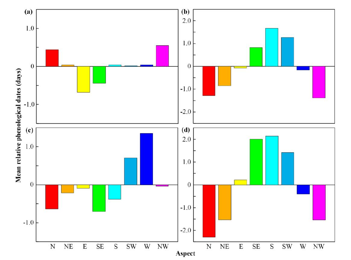
3.1. Effects of Topographical Parameters on Land Surface Phenology at Local Scales

To reveal detailed spatial patterns of Landsat LSP and its relation to topographical parameters, we extracted elevation, aspect, slope, and greenup onset and dormancy onset dates within a 12 × 12 km steppe area in the 17th Landsat zone. In this area, the elevation varies from 4300 to 6250 m (Figure 4a). The earlier greenup dates (125 to 145 DOY) and later dormancy dates (285 to 320 DOY) (i.e., the longer growing season) appeared in the valley where elevation is less than 4400 m and slope is less than 10° (Figure 4a,c,e,f). From the piedmont to the snow line near the mountaintop, the greenup onset tended to be delayed at a rate of 0.54 day/100 m (r = 0.64, p < 0.0001), and dormancy onset tended to advance at a rate of −0.46 day/100 m (r = −0.81, p < 0.0001). However, LSP was undetectable in areas with an elevation above 5600 m, where snow generally covered over the entire year (Figure 4d,e,f). Near the snow line, greenup and dormancy onset usually occurred in mid-July (190 to 200 DOY) and mid-September (250 to 260 DOY) with a growing season duration of less than two months. This pattern clearly demonstrates the strong impacts of elevation on vegetation phenology.

The spatial pattern of aspect also shows the significant impacts on vegetation phenology (Figure 4b,e,f). Taking the Mountains 1, 2, and 3 as examples (Figure 4d), greenup and dormancy onsets on the sunlit slopes (south and southeast) were both about 20–30 days later than those on the shaded slopes (north and northwest).

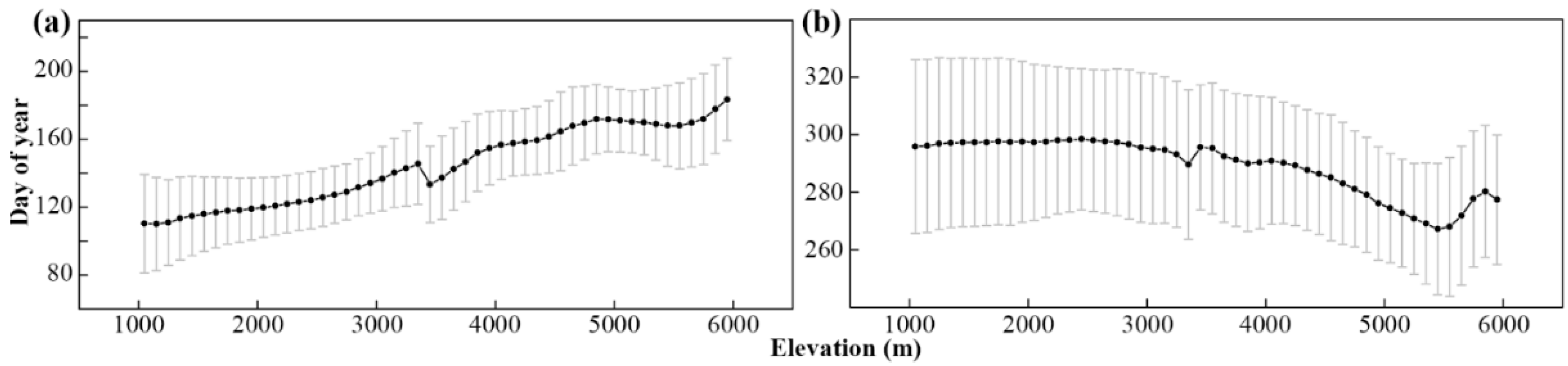
3.2. Effects of Topographical Parameters on Land Surface Phenology at Regional Scales

Figure 5 shows spatial patterns of three-year average greenup onset dates and dormancy onset dates over the 17 zones. Greenup onset dates occurred in late March in eastern regions and irregularly shifted westwards with dates as late as July. In contrast, dormancy onset appeared from early August to late November but did not show an obvious gradient change from east to west.

With respect to relationship between land surface phenology and elevation, the average greenup onset date showed a delayed tendency (p < 0.0001) from low elevation to high elevation, while the average dormancy onset date indicated an advanced tendency (p < 0.0001) from low elevation to high elevation. The gradients of average greenup onset date and average dormancy onset date along elevation from 1000 m to 6000 m were 1.52 days/100 m and −0.59 days/100 m, respectively. It should be noted that phenological progression with the elevation increase was interrupted in some elevation ranges, particularly around 3400 m. In addition, the dormancy onset dates turned to delay at elevations above 5600 m (Figure 6).

To reveal the relationship between land surface phenology and aspect, we calculated the mean relative phenological date for a given aspect (difference between the mean phenological date on a given aspect and the mean phenological date on all aspects across the belt transect of the QTP) in meadow and steppe areas, respectively. For the timing of greenup onset in the meadow area, the relative greenup onset dates were mostly positive on north and northwest slopes (shaded slopes) during 2013 to 2015, indicating a relatively later greenup onset date. In contrast, the relative greenup onset dates were negative on east and southeast slopes (sunlit slopes), indicating a relatively earlier greenup onset date. Specifically, greenup onset was 1 to 2 days earlier on the partially sunlit slopes than on the shaded slopes (Figure 7a). For the timings of dormancy onset in the meadow area however, the earlier dates occurred on north, northeast, and northwest slopes (shaded slopes), while the later dates appeared on southeast, south, and southwest slopes (sunlit slopes). Overall, dormancy onset was about 2–4 days earlier on the shaded slopes than on the sunlit slopes (Figure 7b). According to a variance analysis and Student’s t-test, all of the differences are significant (p < 0.05).

In the steppe area, the positive relative greenup onset dates were mostly found on partially sunlit slopes (southwest and west slopes), while the negative relative greenup onset dates were detected not only on shaded slopes (north and northeast slopes), but also on sunlit slopes (south and southeast slopes) (Figure 7c). Similar to the pattern in the meadow area, dormancy onset on shaded slopes (north, northeast, and northwest) occurred about 3–5 days earlier than that on sunlit slopes (southeast, south, and southwest) (Figure 7d). Based on a variance analysis and Student’s t-test, all of the differences are also significant (p < 0.05).

Considering the effects of the slope on land surface phenology in the meadow area, the mean relative greenup onset date shows nonlinear variation with the slope increase on both north (Figure 8a) and south (Figure 8c) slopes. The relative greenup date remained relatively stable without a significant trend on slopes less than 30°. However, the relative greenup date correlated significantly positively (p < 0.0001) with slope on slopes more than 30° on both north (Figure 8a) and south (Figure 8c) slopes. More specifically, mean relative greenup onset date was delayed with the increase of slope (from 0–50°) at rates of 1.15 (on north slope; p < 0.0001) and 0.72 (on south slope; p < 0.0001) days per 10°. In contrast, mean relative dormancy onset date significantly advanced (p < 0.0001) with the increase of slope at rates of 2.74 (on north slope; Figure 8b) and 0.78 (on south slope; Figure 8d) days per 10°. Overall, as slope increases, greenup and dormancy onset dates change more rapidly on the north slope than on the south slope in the meadow area.

In the steppe area, however, the impact pattern of slope was opposite to that in the meadow area. The mean relative greenup onset date significantly shifted to an earlier date with the increase of slope (p < 0.0001) on both north (Figure 9a) and south (Figure 9c) slopes. The mean changing rates are 3.6 days/10° on the north slope and 5 days/10° on the south slope. The mean relative dormancy onset date is slightly delayed (p > 0.05) with the increase of slope on the north slope (Figure 9b) but significantly delayed (p < 0.0001) with the increase of slope on the south slope (Figure 9d). The mean changing rate on the south slope is 3.44 days/10°. This pattern indicates that greenup and dormancy onset dates changed more rapidly with the increase of slope on the south slope than on the north slope in the steppe area.

4. Discussion

Our research investigated a new approach to detecting vegetation phenology from the Landsat observations in the same year and then quantified the impacts of topographic features at 30 m resolution on the spatial heterogeneity of vegetation phenological metrics. It improved the understanding of vegetation phenology variation on the QTP. Combining Landsat ETM+/OLI observations in overlapping zones of adjacent images offered a high frequency of data for the extraction of land surface phenology. This increase in scene number allowed us to investigate the spatial patterns of vegetation phenology in the same year at a spatial resolution of 30 m in a region spanning 2600 km of the QTP. The reliability of LSP extractions is strongly dependent on the quality of Landsat observations, which is influenced mainly by the number of Landsat overpasses, frequency of cloud contamination, and the Scan Line Corrector (SLC) failure in ETM+. Therefore, to reveal spatial variations of LSP precisely, the evaluation of Landsat observations and phenological extractions is necessary. As the quality of Landsat-derived NDVI data can be measured by PGQ—namely, the higher the PGQ score, the higher the quality of NDVI data—NDVI data in western zones and the central area of each zone should be better than in eastern zones and the edge areas of each zone on the QTP. In this study, we removed NDVI data with the PGQ less than 25% because the LSP with PGQ above 25% is closer to ground-based phenological date observations acquired from the limited ground stations on the QTP. Our study confirmed that PGQ could be used as an important measure of data quality in Landsat-based vegetation phenology extractions. However, PGQ provides an evaluation of overall quality for an EVI2 time series, but it is less likely able to quantify the detection quality of a specific phenological transition date. Indeed, it has been demonstrated that large uncertainties in phenology detections are produced when missing Landsat observations occur around phenological transition dates [48]. Thus, the local proportion of good-quality (LPGQ) observations has been proposed to evaluate the detection quality for each phenological transition date in a vegetation growing cycle [36], which is calculated based on the good-quality observations around the given phenological date. Certainly, LPGQ provides a better evaluation of NDVI data quality around each phenological date in an individual pixel than does PGQ. In this study, however, as topographic impacts on spatial heterogeneity of vegetation phenological metrics were derived by analyzing a large number of pixels at a spatial resolution of 30 m, NDVI data quality around each phenological date is assumed to have only marginal influences on the phenology timing determination.

Based on combined analysis of LSP and elevation, greenup onset is delayed but dormancy onset advances as the elevation increases on the QTP, which is consistent with the results derived from coarse-spatial-resolution satellite data (1–8 km) [10,14,15,19]. However, the changing rates in our study are significantly larger than those in the previous studies (

Table 1. Comparison of elevational gradients of change in LSP derived from different vegetation indices and satellite data.

Source	Data Set	Spatial Resolution	Year	Method	Season	Rate (Days/100 m)
Piao et al., 2011	GIMMS NDVI	8 km	1982–2006	Maximum slope threshold	Spring	+0.7
Ding et al., 2013	SPOT NDVI	1 km	1999–2009	Maximum slope threshold	Spring Autumn	+0.9 −0.1
Che et al., 2014	GIMMS3g LAI	8 km	1982–2011	Curvature change rate	Autumn	−0.3
Shen et al., 2014	GIMMS NDVI, SPOT NDVI, MODIS NDVI/EVI	8 km 1 km	2000–2011	Maximum slope threshold, curvature change rate	Spring	+1.1
This study	Landsat NDVI	30 m	2013–2015	Curvature change rate	Spring Autumn	1.52 −0.59

) because scaling effects may induce larger changing rates at the spatial resolution of 30 m [51]. In other words, the coarser-resolution satellite data may smooth and attenuate the changing rates of LSP. Thus, the elevation dependence of change in land surface phenology detected by Landsat data should be more precise than that derived by AVHRR, MODIS, and SPOT data.

Moreover, the elevational gradient of change in greenup onset date was nearly four times as large as that of dormancy onset (Figure 6), which confirms the conclusion that spring phenology variation is very sensitive to air temperature variation [9,52]. By contrast, the smaller elevational gradient of change in dormancy onset date is likely associated with the strong impacts of both temperature and precipitation [15], because precipitation is less dependent on elevation than air temperature. Meanwhile, interruption of phenological progression at about 3400 m might be associated with abrupt elevation change from Zone 1 to Zone 2 (Figure A2), while the delayed tendency of the dormancy onset date above 5600 m (Figure 6b) may be induced by disturbance of snow cover (see Figure 4d,e,f).

The elevation dependence of vegetation LSP on the QTP has been the research focus for terrain effects; whereas, influences of aspect and slope on LSP have usually been neglected. However, the topographic controls of local vegetation phenology in the mountainous region are integrated by elevation, aspect, and slope. Landsat data with the higher spatial resolution allowed us to detect the impact of terrain on phenology through aspect and slope. To quantify the separate effects of the aspect or slope on the LSP, we used the single variable principle to eliminate the other factors which controlled the LSP. The results confirm that aspect and slope do have strong controls on LSP and the climatic cues are diverse. In the meadow area, greenup onset on shaded slopes was usually later than that on sunlit slopes, which can be explained by lower temperature and later snowmelt timing on the shaded slopes than on the sunlit slopes [50]. Contrarily, the lower temperature on the shaded slopes triggered an earlier occurrence date of dormancy onset, while the higher temperature on the sunlit slopes induced a later occurrence date of dormancy onset (Figure 7a,b). In the steppe area, greenup onset was earlier on both shaded and sunlit slopes (Figure 7c), which indicates that greenup onset may not be mainly affected by air temperature but by precipitation and soil moisture regimes [8]. As the dependence of precipitation on aspect may be smaller than that of temperature in the steppe area where slopes are usually smaller than 30° (Figure 1, Figure A2), the differences in greenup onset dates between shaded and sunlit slopes are not significant. However, similar to the dormancy onset response to aspect in the meadow area, the dormancy onset in the steppe area was also earlier on shaded slopes than on sunlit slopes (Figure 7d), which may be induced by lower temperature. Moreover, the effect of aspect on phenological occurrence dates was larger in the steppe area than in the meadow area, especially for dormancy onset. This finding implies that the response of steppe dormancy onset to temperature regimes might be more sensitive than that of meadow dormancy onset on the QTP, possibly due to the lower levels of moisture in the steppe.

With respect to slope effects on LSP, we detected opposite patterns in meadow and steppe areas (Figure 8 and Figure 9). To analyze the climatic attribution of slope effects on LSP, relationships between slope steepness and microclimatic factors should be identified. Unfortunately, there are no specified meteorological observations on different aspects and slopes of the QTP. Thus, we can only roughly evaluate possible climatic cues of slope effects on LSP. According to microclimatic observations on different aspects and slopes of mountainous areas in southern China [53], soil temperature and evaporation decrease with the increase of slope on the north slope but increase on the south slope. Statistical analysis and process-based modeling of long-term phenological observation data on the QTP showed that herbaceous plant green leaves may not grow until the ground has been warmed above 0 °C after snow melt. Hence, snow-melt water is a crucial factor for triggering greenup in addition to temperature in snow-dominated regions of the QTP [9]. That is, more snowfall during late winter and early spring can translate into more soil moisture storage as spring temperature increases, and induce earlier greenup; whereas, less snowfall during late winter and early spring can limit soil moisture availability under rapid spring temperature increase, and force later greenup. In addition, statistical analysis based on remote sensing data on the QTP indicated that the end date of the growing season (EGS) was also controlled by thermal–moisture conditions. Namely, the higher the monthly mean air temperature and the more the monthly precipitation, the later the EGS [15]. Based on the above microclimatic characteristics and plant phenological responses to climatic factors, we attempt to explain slope effects on LSP.

In the meadow area, the range of slope steepness with effective vegetation phenological data was between 0 and 50 degrees. On the south slope, although soil temperature might be high on the steep slope, strong evaporation may induce soil water deficit and limit the advancing effect of high temperature on greenup onset and delaying effect of high temperature on dormancy onset. Due to predominant effects of soil water deficit on plant phenology on the south slope, later greenup onset and earlier dormancy onset occurred on the steep slope (Figure 8c,d). On the north slope, however, lower soil temperature on the steep slope may play a vital role and result in later greenup onset and earlier dormancy onset (Figure 8a,b). In the steppe area, the climate is drier than in the meadow area. The plant community is mainly composed of meso-xerophytes and xerophytes, such as Stipa and Artemisia. As the range of slope steepness with effective vegetation phenological data was less than in the meadow area (between 0 and 40 degrees), the combination of high soil temperature and strong evaporation on the steep south slope may not induce significant soil water shortage. Under the leading effect of the soil temperature gradient change on plant phenology, earlier greenup onset and later dormancy onset appeared on the steep slope (Figure 9c,d). On the north slope, the range of soil temperature and evaporation decrease with the increase of slope might be also less than that in the meadow area, and result in a slightly lower soil temperature but relatively higher soil moisture on the steep slope. Under the leading effect of the soil moisture gradient change on plant phenology, greenup onset shifted to an earlier date and dormancy onset was postponed slightly with the increase of slope (Figure 9a,b).

5. Conclusions

This study has realized high-precision extraction of vegetation phenology through combining Landsat ETM+/OLI observations in overlapping zones of adjacent images from 2013 to 2015, and revealed terrain effects on land surface phenology along a 2600 km belt transect on the QTP. This approach is of crucial importance for accurately estimating phenological performance under complex terrain conditions. The main conclusions are as follows.

Within a 12 × 12 km steppe area, spatial patterns of greenup onset and dormancy onset dates were controlled mainly by elevation and aspect. At regional scales, the greenup onset date showed a delayed tendency with the increase of elevation at a mean rate of 1.52 days/100 m, while the dormancy onset date indicated an advanced tendency at a mean rate of −0.59 days/100 m. The elevation dependence of change in land surface phenology detected by Landsat data in our study is significantly larger and more precise than those derived from AVHRR, MODIS, and SPOT data in the previous studies. In the meadow area, greenup onset date was usually later but dormancy onset date was commonly earlier on shaded slopes than on sunlit slopes. The main attribution of phenological timing distribution on different aspects might be temperature regimes. By contrast, greenup onset date in the steppe area did not significantly depend on aspects. Precipitation and soil moisture regimes may play a role in causing greenup onset timing distribution on different aspects. However, dormancy onset date in the steppe area indicated a similar response to aspects with that in the meadow area. With regard to the effect of slope on vegetation phenology in the meadow area, greenup onset date was significantly delayed but dormancy onset date significantly advanced with the increase of slope on both north and south slopes. Either delaying rate in greenup onset or advancing rate in dormancy onset was more rapid on the north slope than on the south slope. In the steppe area, however, greenup onset significantly shifted to an earlier date with the increase of slope on both north and south slopes, while dormancy onset was significantly postponed with the increase of slope only on the south slopes. The advancing rate in greenup onset and delaying rate in dormancy onset were more rapid on the south slope than on the north slope. The coordination status of temperature and moisture on different aspects with the increase of slope controls gradient changes of spring and autumn phenology.

References

1. Schwartz, D.M.; Chen, X.; Keatley, R.M.; Chambers, E.L.; Phillips, R.; Menzel, A.; Beaubien, G.E.; Crimmins, M.T.; Weltzin, F.J.; Morellato, C.L.P.C.; et al. Phenology: An Integrative Environmental Science, 2nd ed.; Springer: Dordrecht, The Netherlands; Heidelberg, Germany; New York, NY, USA; London, UK, 2013. [Google Scholar]
2. Chen, X.Q. Spatiotemporal Processes of Plant Phenology Simulation and Prediction; Springer Nature: Berlin, Germany, 2017. [Google Scholar]
3. Richardson, A.D.; Keenan, T.F.; Migliavacca, M.; Ryu, Y.; Sonnentag, O.; Toomey, M. Climate change, phenology, and phenological control of vegetation feedbacks to the climate system. Agric. For. Meteorol. 2013, 169, 156–173. [Google Scholar] [CrossRef]
4. Chen, H.; Zhu, Q.; Peng, C.; Wu, N.; Wang, Y.; Fang, X.; Gao, Y.; Zhu, D.; Yang, G.; Tian, J.; et al. The impacts of climate change and human activities on biogeochemical cycles on the Qinghai–Tibetan Plateau. Glob. Chang. Biol. 2013, 19, 2940–2955. [Google Scholar] [CrossRef] [PubMed]
5. Yu, H.; Luedeling, E.; Xu, J. Winter and spring warming result in delayed spring phenology on the Tibetan Plateau. Proc. Natl. Acad. Sci. USA 2010, 107, 22151–22156. [Google Scholar] [CrossRef] [PubMed] [Green Version]
6. Zhang, G.; Zhang, Y.; Dong, J.; Xiao, X. Green-up dates in the Tibetan Plateau have continuously advanced from 1982 to 2011. Proc. Natl. Acad. Sci. USA 2013, 110, 4309–4314. [Google Scholar] [CrossRef] [PubMed] [Green Version]
7. Shen, M.; Piao, S.; Chen, X.; An, S.; Fu, Y.H.; Wang, S.; Cong, N.; Janssens, I.A. Strong impacts of daily minimum temperature on the green-up date and summer greenness of the Tibetan Plateau. Glob. Chang. Biol. 2016, 22, 3057–3066. [Google Scholar] [CrossRef] [PubMed]
8. Shen, M.; Piao, S.; Cong, N.; Zhang, G.; Jassens, I.A. Precipitation impacts on vegetation spring phenology on the Tibetan Plateau. Glob. Chang. Biol. 2015, 21, 3647–3656. [Google Scholar] [CrossRef] [PubMed] [Green Version]
9. Chen, X.; An, S.; Inouye, D.W.; Schwartz, M.D. Temperature and snowfall trigger alpine vegetation green-up on the world’s roof. Glob. Chang. Biol. 2015, 21, 3635–3646. [Google Scholar] [CrossRef] [PubMed]
10. Piao, S.; Cui, M.; Chen, A.; Wang, X.; Ciais, P.; Liu, J.; Tang, Y. Altitude and temperature dependence of change in the spring vegetation green-up date from 1982 to 2006 in the Qinghai–Xizang Plateau. Agric. For. Meteorol. 2011, 151, 1599–1608. [Google Scholar] [CrossRef]
11. Shen, M.; Tang, Y.; Chen, J.; Zhu, X.; Zheng, Y. Influences of temperature and precipitation before the growing season on spring phenology in grasslands of the central and eastern Qinghai–Tibetan Plateau. Agric. For. Meteorol. 2011, 151, 1711–1722. [Google Scholar] [CrossRef]
12. Yu, H.; Xu, J.; Okuto, E.; Luedeling, E. Seasonal response of grasslands to climate change on the Tibetan Plateau. PLoS ONE 2012, 7, e49230. [Google Scholar] [CrossRef] [PubMed]
13. Shrestha, U.B.; Gautam, S.; Bawa, K.S. Widespread climate change in the Himalayas and associated changes in local ecosystems. PLoS ONE 2012, 7, e36741. [Google Scholar] [CrossRef] [PubMed] [Green Version]
14. Shen, M.; Zhang, G.; Cong, N.; Wang, S.; Kong, W.; Piao, S. Increasing altitudinal gradient of spring vegetation phenology during the last decade on the Qinghai–Tibetan Plateau. Agric. For. Meteorol. 2014, 189–190, 71–80. [Google Scholar] [CrossRef]
15. Che, M.; Chen, B.; Innes, J.L.; Wang, G.; Dou, X.; Zhou, T.; Zhang, H.; Yan, J.; Xu, G.; Zhao, H. Spatial and temporal variations in the end date of the vegetation growing season throughout the Qinghai–Tibetan Plateau from 1982 to 2011. Agric. For. Meteorol. 2014, 189–190, 81–90. [Google Scholar] [CrossRef]
16. Ding, M.; Chen, Q.; Li, L.; Zhang, Y.; Wang, Z.; Liu, L.; Sun, X. Temperature dependence of variations in the end of the growing season from 1982 to 2012 on the Qinghai–Tibetan Plateau. GISci. Remote Sens. 2015, 53, 147–163. [Google Scholar] [CrossRef]
17. Cong, N.; Shen, M.; Yang, W.; Yang, Z.; Zhang, G.; Piao, S. Varying responses of vegetation activity to climate changes on the Tibetan Plateau grassland. Int. J. Biometeorol. 2017, 61, 1433–1444. [Google Scholar] [CrossRef] [PubMed]
18. Wang, C.; Guo, H.; Zhang, L.; Liu, S.; Qiu, Y.; Sun, Z. Assessing phenological change and climatic control of alpine grasslands in the Tibetan Plateau with MODIS time series. Int. J. Biometeorol. 2015, 59, 11–23. [Google Scholar] [CrossRef] [PubMed]
19. Ding, M.; Zhang, Y.; Sun, X.; Liu, L.; Wang, Z.; Bai, W. Spatiotemporal variation in alpine grassland phenology in the Qinghai–Tibetan Plateau from 1999 to 2009. Chin. Sci. Bull. 2012, 58, 396–405. [Google Scholar] [CrossRef]
20. Liu, X.; Zhu, X.; Zhu, W.; Pan, Y.; Zhang, C.; Zhang, D. Changes in spring phenology in the Three-Rivers headwater region from 1999 to 2013. Remote Sens. 2014, 6, 9130–9144. [Google Scholar] [CrossRef]
21. Cong, N.; Shen, M.; Piao, S.; Chen, X.; An, S.; Yang, W.; Fu, Y.H.; Meng, F.; Wang, T. Little change in heat requirement for vegetation green-up on the Tibetan Plateau over the warming period of 1998–2012. Agric. For. Meteorol. 2017, 232, 650–658. [Google Scholar] [CrossRef]
22. Hwang, T.; Song, C.; Bolstad, P.V.; Band, L.E. Downscaling real-time vegetation dynamics by fusing multi-temporal MODIS and Landsat NDVI in topographically complex terrain. Remote Sens. Environ. 2011, 115, 2499–2512. [Google Scholar] [CrossRef]
23. Hwang, T.; Song, C.; Vose, M.J.; Band, E.L. Topography-mediated controls on local vegetation phenology estimated from modis vegetation index. Landsc. Ecol. 2011, 26, 541–556. [Google Scholar] [CrossRef]
24. Day, F.P.; Philips, D.L.; Monk, C.D. Forest Hydrology and Ecology at Coweeta; Springer: New York, NY, USA, 1988. [Google Scholar]
25. Yang, K.; He, J.; Tang, W.; Qin, J.; Cheng, C.C.K. On downward shortwave and longwave radiations over high altitude regions: Observation and modeling in the Tibetan Plateau. Agric. For. Meteorol. 2010, 150, 38–46. [Google Scholar] [CrossRef]
26. Ju, J.; Roy, D.P. The availability of cloud-free landsat etm+ data over the conterminous United States and globally. Remote Sens. Environ. 2008, 112, 1196–1211. [Google Scholar] [CrossRef]
27. Fisher, J.; Mustard, J.; Vadeboncoeur, M. Green leaf phenology at Landsat resolution: Scaling from the field to the satellite. Remote Sens. Environ. 2006, 100, 265–279. [Google Scholar] [CrossRef]
28. Fisher, J.I.; Mustard, J.F. Cross-scalar satellite phenology from ground, Landsat, and MODIS data. Remote Sens. Environ. 2007, 109, 261–273. [Google Scholar] [CrossRef]
29. Melaas, E.K.; Friedl, M.A.; Zhu, Z. Detecting interannual variation in deciduous broadleaf forest phenology using Landsat TM/ETM+ data. Remote Sens. Environ. 2013, 132, 176–185. [Google Scholar] [CrossRef]
30. Melaas, E.K.; Sulla-Menashe, D.; Gray, J.M.; Black, T.A.; Morin, T.H.; Richardson, A.D.; Friedl, M.A. Multisite analysis of land surface phenology in North American temperate and boreal deciduous forests from Landsat. Remote Sens. Environ. 2016, 186, 452–464. [Google Scholar] [CrossRef]
31. Nijland, W.; Bolton, D.K.; Coops, N.C.; Stenhouse, G. Imaging phenology; scaling from camera plots to landscapes. Remote Sens. Environ. 2016, 177, 13–20. [Google Scholar] [CrossRef]
32. Walker, J.J.; de Beurs, K.M.; Wynne, R.H.; Gao, F. Evaluation of Landsat and MODIS data fusion products for analysis of dryland forest phenology. Remote Sens. Environ. 2012, 117, 381–393. [Google Scholar] [CrossRef]
33. Gao, F.; Anderson, M.C.; Zhang, X.; Yang, Z.; Alfieri, J.G.; Kustas, W.P.; Mueller, R.; Johnson, D.M.; Prueger, J.H. Toward mapping crop progress at field scales through fusion of Landsat and MODIS imagery. Remote Sens. Environ. 2017, 188, 9–25. [Google Scholar] [CrossRef]
34. Walker, J.J.; de Beurs, K.M.; Wynne, R.H. Dryland vegetation phenology across an elevation gradient in Arizona, USA, investigated with fused MODIS and Landsat data. Remote Sens. Environ. 2014, 144, 85–97. [Google Scholar] [CrossRef]
35. Zhu, X.; Chen, J.; Gao, F.; Chen, X.; Masek, J.G. An enhanced spatial and temporal adaptive reflectance fusion model for complex heterogeneous regions. Remote Sens. Environ. 2010, 114, 2610–2623. [Google Scholar] [CrossRef]
36. Zhang, X.; Friedl, M.A.; Schaaf, C.B. Sensitivity of vegetation phenology detection to the temporal resolution of satellite data. Int. J. Remote Sens. 2009, 30, 2061–2074. [Google Scholar] [CrossRef]
37. Domrös, M.; Peng, G. The Climate of China; Springer: Berlin, Germany, 1988. [Google Scholar]
38. Hou, X. (Ed.) Editorial Board of Vegetation Map of China CAS 1:1000,000 Vegetation Atlas of China; Science Press: Beijing, China, 2001. [Google Scholar]
39. Masek, J.G.; Vermote, E.F.; Saleous, N.E.; Wolfe, R.; Hall, F.G.; Huemmrich, K.F.; Gao, F.; Kutler, J.; Lim, T.K. A Landsat surface reflectance dataset for North America, 1990–2000. IEEE Geosci. Remote Sen. Lett. 2006, 3, 68–72. [Google Scholar] [CrossRef]
40. Vermote, E.F.; El Saleous, N.; Justice, C.O.; Kaufman, Y.J.; Privette, J.L.; Remer, L.; Roger, J.C.; Tanré, D. Atmospheric correction of visible to middle-infrared EOS-MODIS data over land surfaces: Background, operational algorithm and validation. J. Geophys. Res. Atmos. 1997, 102, 17131–17141. [Google Scholar] [CrossRef] [Green Version]
41. Zhu, Z.; Wang, S.; Woodcock, C.E. Improvement and expansion of the Fmask algorithm: Cloud, cloud shadow, and snow detection for Landsats 4–7, 8, and Sentinel 2 images. Remote Sens. Environ. 2015, 159, 269–277. [Google Scholar] [CrossRef]
42. Zhu, Z.; Woodcock, C.E. Object-based cloud and cloud shadow detection in Landsat imagery. Remote Sens. Environ. 2012, 118, 83–94. [Google Scholar] [CrossRef]
43. Roy, D.P.; Kovalskyy, V.; Zhang, H.K.; Vermote, E.F.; Yan, L.; Kumar, S.S.; Egorov, A. Characterization of Landsat-7 to Landsat-8 reflective wavelength and normalized difference vegetation index continuity. Remote Sens. Environ. 2016, 185, 57–70. [Google Scholar] [CrossRef]
44. Zhang, X. Reconstruction of a complete global time series of daily vegetation index trajectory from long-term AVHRR data. Remote Sens. Environ. 2015, 156, 457–472. [Google Scholar] [CrossRef]
45. Zhang, X.; Friedl, M.A.; Schaaf, C.B.; Strahler, A.H.; Hodges, J.C.F.; Gao, F.; Reed, B.C.; Huete, A. Monitoring vegetation phenology using MODIS. Remote Sens. Environ. 2003, 84, 471–475. [Google Scholar] [CrossRef]
46. Elmore, A.J.; Guinn, S.M.; Minsley, B.J.; Richardson, A.D. Landscape controls on the timing of spring, autumn, and growing season length in Mid-Atlantic forests. Glob. Chang. Biol. 2012, 18, 656–674. [Google Scholar] [CrossRef]
47. Zhang, X.; Jayavelu, S.; Liu, L.; Friedl, M.A.; Henebry, G.M.; Liu, Y.; Schaaf, C.B.; Richardson, A.D.; Gray, J. Evaluation of land surface phenology from VIIRS data using time series of phenocam imagery. Agric. For. Meteorol. 2018, 256–257, 137–149. [Google Scholar] [CrossRef]
48. Zhang, X.; Liu, L.; Yan, D. Comparisons of global land surface seasonality and phenology derived from AVHRR, MODIS, and VIIRS data. J. Geophys. Res. Biogeosci. 2017, 122, 1506–1525. [Google Scholar] [CrossRef]
49. Willmott, C.J. On the validation of models. Phys. Geogr. 1981, 2, 184–194. [Google Scholar]
50. Chen, W.N.; Wang, H.; Xiao, X.J.; Chen, F.J.; Zhang, Z.Y.; Qi, Z.M.; Huang, Z.X. Effects of slope aspect on growth and reproduction of Fritillaria unibracteata (liliaceae). Acta Ecol. Sin. 2016, 36, 1–9. (In Chinese) [Google Scholar]
51. Zhang, X.; Wang, J.; Gao, F.; Liu, Y.; Schaaf, C.; Friedl, M.; Yu, Y.; Jayavelu, S.; Gray, J.; Liu, L.; et al. Exploration of scaling effects on coarse resolution land surface phenology. Remote Sens. Environ. 2017, 190, 318–330. [Google Scholar] [CrossRef]
52. Liu, L.; Liu, L.; Liang, L.; Donnelly, A.; Park, I.; Schwartz, M.D. Effects of elevation on spring phenological sensitivity to temperature in Tibetan Plateau grasslands. Chin. Sci. Bull. 2014, 59, 4856–4863. [Google Scholar] [CrossRef]
53. Fu, B.P. Mountain Climate; Science Press: Beijing, China, 1983. (In Chinese) [Google Scholar]
Figure 1. Distribution of meadow and steppe on the Qinghai–Tibet Plateau. The squares denote the Landsat scenes and their overlapping zones along an east–west transect across the middle of the Qinghai–Tibet Plateau.
Remotesensing 10 01069 g001
Figure 2. Fitting of temporal Normalized Difference Vegetation Index (NDVI) trajectory and extraction of phenological dates from 2013 to 2015 at an arbitrary pixel in the meadow area (a) and the steppe area (b), respectively. The green plus sign denotes Landsat 7 ETM+ (Enhanced Thematic Mapper Plus) NDVI. The yellow plus sign denotes Landsat 8 OLI (Operational Land Imager) NDVI. The solid curve represents the fitted NDVI.
Remotesensing 10 01069 g002
Figure 3. Spatial patterns of the average proportion of good-quality observations (PGQ) and the average index of agreement (d) of Hybrid Piecewise Logistic Model (HPLM) fitting of NDVI curves across the 17 zones during 2013 to 2015. The PGQ for pixels without continuous observations in one month were set to 0.
Remotesensing 10 01069 g003
Figure 4. Spatial patterns of topographical parameters and Landsat land surface phenology (LSP) within a 12 × 12 km area of steppe in Zone 17. (a) Elevation (m); (b) aspect (F, N, NE, E, SE, S, SW, W, and NW denote flat, north, northeast, east, southeast, south, southwest, west, and northwest slopes, respectively); (c) slope (°); (d) Google Earth high-resolution image (spatial resolution: 2.5 m) on 3 June 2013 (where numbers 1, 2, and 3 represent three mountains with sunlit slopes and corresponding shaded slopes); (e) greenup onset date (DOY) in 2015; and (f) dormancy onset date (DOY) in 2015.
Remotesensing 10 01069 g004
Figure 5. Spatial patterns of Landsat-derived average greenup onset date (GO) and dormancy onset date (DO) during 2013 to 2015.
Remotesensing 10 01069 g005
Figure 6. Changes in average greenup onset date (a) and average dormancy onset date (b) along the elevation gradient on the QTP during 2013–2015 (three-year average value). Solid lines denote the average phenological dates at given elevations (interval = 100 m). Error bars denote the standard deviations of phenological dates at given elevations.
Remotesensing 10 01069 g006
Figure 7. Mean relative phenological dates on different aspects for greenup onset (a) and dormancy onset (b) in the meadow area and for greenup onset (c) and dormancy onset (d) in the steppe area during 2013 to 2015 (three-year average value). N, NE, E, SE, S, SW, W, and NW represent north, northeast, east, southeast, south, southwest, west, and northwest aspect slopes, respectively.
Remotesensing 10 01069 g007
Figure 8. Changes in mean relative greenup onset and dormancy onset dates during 2013–2015 (three-year average value) along the slope gradient on the north (a,b) and south (c,d) slopes in the meadow area. Dotted lines represent mean relative phenological dates at given slopes (interval = 1°). Error bars denote the standard deviations of relative phenological dates at given slopes.
Remotesensing 10 01069 g008
Figure 9. Changes in mean relative greenup onset and dormancy onset dates during 2013–2015 (three-year average value) along the slope gradient on the north (a,b) and south (c,d) slopes in the steppe area. Dotted lines represent mean relative phenological dates at given slopes (interval = 1°). Error bars denote the standard deviations of relative phenological dates at given slopes.
Remotesensing 10 01069 g009