Abstract
An intercalibrated Fundamental Climate Data Record (FCDR) of brightness temperatures (Tb) has been developed using data from a total of 14 research and operational conical-scanning microwave imagers. This dataset provides a consistent 30+ year data record of global observations that is well suited for retrieving estimates of precipitation, total precipitable water, cloud liquid water, ocean surface wind speed, sea ice extent and concentration, snow cover, soil moisture, and land surface emissivity. An initial FCDR was developed for a series of ten Special Sensor Microwave/Imager (SSM/I) and Special Sensor Microwave Imager Sounder (SSMIS) instruments on board the Defense Meteorological Satellite Program spacecraft. An updated version of this dataset, including additional NASA and Japanese sensors, has been developed as part of the Global Precipitation Measurement (GPM) mission. The FCDR development efforts involved quality control of the original data, geolocation corrections, calibration corrections to account for cross-track and time-dependent calibration errors, and intercalibration to ensure consistency with the calibration reference. Both the initial SSMI(S) and subsequent GPM Level 1C FCDR datasets are documented, updated in near real-time, and publicly distributed.
1. Introduction
The launch of the Special Sensor Microwave/Imager (SSM/I) on board the Defense Meteorological Satellite Program’s (DMSP) F08 spacecraft in June of 1987 marked the beginning of a nearly continuous long-term record of high-quality global satellite microwave observations, which now extends over 30 years. The long time series provided by these operational sensors along with their frequent sampling, global coverage, stability, and sensitivity makes these data extremely valuable for global water cycle studies. The SSM/I and succeeding Special Sensor Microwave Imager Sounder (SSMIS) window channels are sensitive to emission by water vapor, cloud water, and precipitating hydrometeors, as well as scattering by large liquid and ice particles, although unlike visible and infrared observations, non-precipitating clouds are relatively transparent at these microwave frequencies. This makes these data well suited for estimates of precipitation rate, column water vapor, and cloud liquid water, as well as surface parameters such as ocean surface wind speed, sea ice extent and concentration, snow cover, soil moisture, and land surface emissivity. The operational focus of these sensors, however, limits their use for many climate applications.
To maximize the use of these data for long-term monitoring, the National Oceanographic and Atmospheric Administration (NOAA) funded the development of a Fundamental Climate Data Record (FCDR) of intercalibrated brightness temperature (Tb) data from the DMSP SSM/I and SSMIS radiometers. The National Research Council [1] defines an FCDR as “sensor data (e.g., calibrated radiances, brightness temperatures, radar backscatter) that have been improved and quality controlled over time, together with the ancillary data used to calibrate them”. SSM/I has seven channels at four frequencies (19.35, 22.235, 37.0, and 85.5 GHz), each of which has both vertically and horizontally polarized channels, except for 22 GHz, which has only vertical polarization. SSMIS has the same seven channels, although the 85.5 GHz frequency was moved to 91.655 GHz. It also has additional temperature and water vapor sounding channels in the 50–60 GHz oxygen absorption band, and near the 183 GHz water vapor line for a total of 24 channels.
A subsequent effort funded under the NASA Precipitation Measurement Missions (PMM) focused on developing an intercalibrated Level 1C dataset for the Global Precipitation Measurement (GPM) mission radiometer constellation. Although this Level 1C FCDR originally involved only the available microwave radiometers starting with the launch of the GPM core satellite in February of 2014, it was subsequently extended to include the Tropical Rainfall Measuring Mission (TRMM) microwave imager (TMI) and associated constellation radiometers, and finally to include the early DMSP SSM/I radiometers. This dataset includes all of the DMSP SSM/I and SSMIS radiometers, as well as additional microwave imagers from NASA and the Japanese Aerospace Exploration Agency (JAXA).
2. Materials and Methods
2.1. DMSP SSMI(S) FCDR
An initial effort to create an intercalibrated Fundamental Climate Data Record focused on microwave imagers from the series of DMSP spacecraft. The seven-channel SSM/I was launched on the DMSP F08 in June of 1987 with five additional copies launched on the DMSP F10, F11, F13, F14, and F15. The next generation SSMIS was launched on the DMSP F16, F17, F18, and F19. DMSP F20 with a fifth copy of the SSMIS instrument was built, but never launched. The available data record from this series of 10 DMSP microwave radiometers is shown in Figure 1.
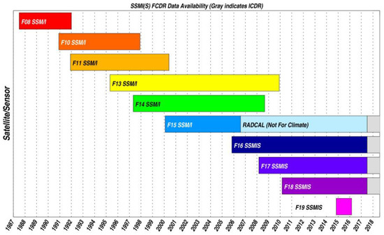
Figure 1.
The availability of SSMI(S) FCDR data from the series of ten DMSP conical-scanning imaging radiometers. The gray shaded portion of the bars indicates ICDR or interim data availability for those sensors continuing to operate. A radar calibration (RADCAL) beacon was turned on in August of 2006 on F15, which substantially impacted the 22 GHz Tb, and F19 lost communications a bit over a year after the SSMIS data became operational. Corrections have been applied for the RADCAL affected F15 data, but significant residual errors remain making it unsuitable for climate applications.
The SSMI(S) FCDR development involved quality control of the data, corrections for cross-track biases, view angle and geolocation errors, emissive reflector issues, solar and lunar intrusions into the warm load, antenna pattern spillover effects, and intercalibration of the instruments [2,3,4,5,6,7,8]. The SSMI(S) FCDR files are output in NetCDF4, with one file per orbit, which starts as the ascending pass of the satellite crosses the equator. It is updated in near real-time with an Interim Climate Data Record (ICDR) for the currently operational sensors, indicated by the gray bars in Figure 1. The same corrections are applied to the ICDR data as for the FCDR data, but no verification of the data has been done. Once the data have been verified and updated corrections and quality flagging have been applied, the data is reprocessed and added to the FCDR data record. The data are available from both NOAA (https://www.ncdc.noaa.gov/cdr/fundamental/ssmis-brightness-temperature-csu) and from Colorado State University (http://rain.atmos.colostate.edu/FCDR). The SSMI(S) FCDR was originally released in early 2013 and the ICDR files are converted to FCDR files on an annual basis after the data are verified and any issues or problems with the interim files are addressed. The total data volume for the complete data record from all ten sensors is ~5.6 terabytes as of May 2018.
The SSMIS FCDR files include the temperature and water vapor sounding channels; however, the sounding channel data are only included in the SSMI(S) FCDR dataset for convenience. The calibration corrections and intercalibration adjustments are only applied to the seven window channels corresponding to those on SSM/I. For the seven FCDR channels, all ten sensors were intercalibrated using SSM/I on board F13 as the calibration reference. F13 was chosen as the reference sensor due to its long life, stable calibration, and minimal change in the equatorial crossing time due to orbit drift. None of the DMSP spacecraft are in controlled orbits, so the orbits decay over time with a gradual decrease in altitude due to atmospheric drag. This results in a change in the local observing time for the sun-synchronous orbits. Unlike the GPM microwave imager (GMI) instrument discussed in the next section, the F13 SSM/I is not assumed to provide a high-quality absolute calibration reference. This means the SSMI(S) FCDR dataset is intercalibrated for consistency (i.e., precision), not to any absolute standard (i.e., accuracy), as a high-quality reference standard was not available at the time.
2.2. Level 1C FCDR
The GPM mission is a constellation-based mission designed to measure precipitation over the globe utilizing available research and operational microwave radiometers to provide high-quality, high temporal resolution precipitation estimates [9,10]. The core GPM satellite was launched in February 2014, with dual-frequency precipitation radars and a 13-channel conical-scanning microwave radiometer. The GPM GMI radiometer was specifically designed as a calibration reference standard to be used to intercalibrate the observed Tb from other available satellite passive microwave radiometers. Data from a series of on-orbit maneuvers was used to identify and develop corrections for GMI calibration issues and to refine the pre-launch spillover corrections independent of radiative transfer models. As a result of the design and both pre and post-launch calibration characterization, the accuracy and stability of the GMI calibration makes it an excellent absolute calibration reference for the radiometer constellation [11,12].
For the radiometer constellation, the need to have consistent Tb between constellation sensors with different specifications and calibrations was recognized early on. To address this issue, an intercalibration working group, also referred to as the XCAL team, was formed within the Precipitation Measurement Missions (PMM) science team, which encompasses both the TRMM and GPM missions. The XCAL team was given responsibility for a “Level 1C” dataset, which is the input for the precipitation retrieval algorithm. This Level 1C dataset differs from the calibrated Level 1B Tb provided by the individual instrument teams by intercalibrating the Tb to a consistent reference standard. This intercalibration accounts for sensor differences, including frequency, polarization, spectral band width, view angle etc., to produce Tb that are physically consistent, but not necessarily identical. After the GMI calibration was finalized, the XCAL team focused on intercalibrating the GPM constellation radiometers including the SSMIS radiometers on board the DMSP F16, F17, F18, and F19 spacecraft, the Advanced Microwave Scanning Radiometer 2 (AMSR2) on board the Japanese Global Change Observation Mission—Water (GCOM-W1) satellite, and the TRMM TMI [12]. Multiple techniques were used to quantify intercalibration differences over both cold ocean scenes and warm vegetated unpolarized land scenes, resulting in typical differences of 2–3 K and maximum differences of up to 5 K. Based on the experience of the on-orbit assessments of the GMI spillover corrections, it is likely that a significant portion of these calibration differences is the result of large uncertainties in the pre-launch measured antenna patterns [12]. After the XCAL team completed the intercalibration of the GPM constellation radiometers for the period from February of 2014 forward and the Level 1C data and subsequent precipitation products were released, the PMM science team focused on updating and reprocessing the TRMM data to develop a long-term consistent precipitation data record extending from December of 1997 to the present. As part of this effort, the XCAL team worked to update the calibration corrections for TRMM TMI [13,14,15], intercalibrate TMI to version V05 of the GMI Tb, and then incorporate the available TRMM-era constellation radiometers by intercalibrating them to GMI [16]. The decision was then made to extend the intercalibrated Level 1C data record further back to the pre-TRMM era SSM/I instruments started with SSM/I on board DMSP F08 in July of 1987. The calibration of the early SSM/I instruments was updated from the earlier SSMI(S) FCDR calibration discussed above. Details of these updates are discussed in the following section.
Figure 2 shows the availability of Level 1C data for the fourteen available conical-scanning radiometers over the 30+year data record starting with the F08 SSM/I in 1987. The dark and light gray shaded regions indicate the GPM and TRMM era sensors. Note that unlike the SSMI(S) FCDR, RADCAL affected F15 SSM/I data after August of 2006 is not included in the Level 1C dataset. Table 1 provides the frequency and polarization of the conical-scanning radiometers included in the Level 1C dataset. The original SSMI(S) FCDR is indicated by the light gray shaded boxes, with the dark gray shading indicating the intercalibrated channels included in the Level 1C dataset. The 6.9 and 7.3 GHz channels of the GCOM-W1 AMSR2 and earlier AMSR-E on board the Earth Observing System (EOS) Aqua satellite are not included with the Level 1C data, as they are not currently used for precipitation retrievals. The Level 1C dataset includes several additional radiometers (i.e., TMI, AMSR-E, AMSR2 and GMI) that are not part of the original SSMI(S) FCDR. These are all newer designs with additional channels and improved spatial resolution, and they are all in controlled orbits. Other updates and improvements to the Level 1C data from the SSMI(S) FCDR include the use of GMI as the calibration reference, intercalibration adjustments as a function of scene temperature, and improvements to the various calibration corrections. All of the Level 1C data are available from the NASA Precipitation Processing System (https://pmm.nasa.gov/data-access/downloads/gpm).
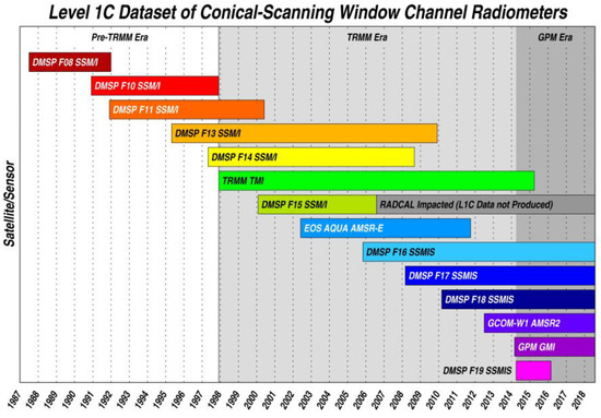
Figure 2.
The availability of Level 1C data from a total of 14 conical-scanning microwave imagers. The light gray shaded region corresponds to the TRMM era and the dark gray region to the GPM era.

Table 1.
Frequency and polarization (v = vertical, h = horizontal) of channels for radiometers in the FCDR datasets. The light gray shading indicates sensors/channels in the original SSMI(S) FCDR. The dark gray shading indicates the additional intercalibrated channels included in the Level 1C dataset. The 6.9 and 7.3 GHz channels on AMSR-E and AMSR2 are not included in the Level 1C dataset.
3. Results
3.1. Updates to the SSM/I Calibration
For the Level 1C dataset, several updates were made to the corrections and calibration adjustments for the six SSM/I instruments from the original SSMI(S) FCDR. This work was done to extend the Level 1C data back to SSM/I on board DMSP F08 in July of 1987 in a manner that is fully consistent with the TRMM and GPM-era radiometers shown in Figure 2. Since this work was just completed and has not been published elsewhere, details of the updated SSM/I corrections including the cross-track bias corrections, geolocation and view angle updates, as well as the intercalibration, are provided in the following section. Note that several aspects of the original SSMI(S) FCDR including the quality control, antenna pattern corrections, updates to the spacecraft ephemeris, etc. remain unchanged.
3.1.1. Cross-Scan Biases
An analysis of the F08 to F14 SSM/I instruments [17] found deviations near the edges of the scan, with a significant decrease in the Tb of 1.5–2.0 K near the right edge for all instruments. The reason for this decrease is due to an obstruction by the spacecraft and/or cold-space mirror partially intruding into the field-of-view. In the initial version of the SSMI(S) FCDR, a multiplicative correction for this falloff was applied based on an analysis of mean, clear-sky antenna temperatures over ocean. This correction, however, did not take into account the effect of instrument mount offsets. An offset in the spacecraft roll direction will impart an asymmetric slope in the antenna temperatures across the scan, while an offset in the spacecraft pitch direction will result in a symmetric curvature across the scan [4]. These effects are most evident over ocean for the lower frequency (i.e., 19, 22, 37 GHz) vertically-polarized (v-pol) channels due to the significant change in Tb with view angle.
To account for these effects, differences between the mean observed and simulated cross-scan Tb were computed for each sensor and channel. The top panel in Figure 3 shows the resulting cross-scan pattern (blue line) for the 19 GHz vertically-polarized channel on the F10 SSM/I. The results for this channel are shown, as they clearly exhibit a left to right slope across the center of the scan associated with an offset in the roll direction, as well as a slight downward curvature, corresponding to a negative pitch. In this case, a roll of −0.08 and a pitch of −0.10, based on simulated Tb, are fit to the center part of the scan (black dots) in order to avoid the edge of scan falloff. The resulting fit is shown by the solid black line. Note that this fit corresponds to a mean roll and pitch value derived using the 19v, 22v, and 37v channels over a 2-year period. For each satellite, the results were checked for consistency between two different years and for the three low-frequency v-pol channels. In all cases, variations in the derived roll and pitch values between channels/years were within a few hundredths of a degree. The final roll and pitch values derived from the cross-scan analysis are given for each sensor in Table 2.
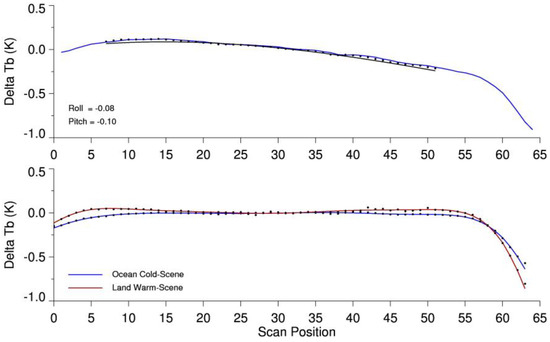
Figure 3.
Observed minus simulated Tb as a function of scan position for the F10 19v channel averaged over 1992 and 1996. The top panel shows the original cross-scan bias in blue, with the dots indicating the position values used to derive the roll and pitch offsets. The resulting fit to roll and pitch is shown by the solid black line with the mean roll and pitch values given in the lower left. The bottom panel shows the cold (Blue) and warm (Red) scene cross-track bias after accounting for the roll and pitch offsets. The cross-track bias correction is derived based on these curves using the equation from [15].
Table 2.
Roll, pitch, yaw and half-cone angle offsets in degrees derived from the cross-scan bias and geolocation analysis for each of the SSM/I instruments.
Once the mean roll and pitch offsets were determined, the data were reprocessed for each sensor to provide updated view angles, or Earth incidence angles (EIA), accounting for the roll and pitch offsets. Observed minus simulated Tb were then recomputed across the scan both over cold ocean scenes and over warm vegetated land scenes. The resulting cross-scan bias patterns are shown in the lower panel in Figure 3. There are slight differences between the cold and warm results, with the most significant being a larger falloff on the right side of the scan at warmer temperatures. This is consistent with the results found for TRMM TMI [15], indicating a fraction of the signal near the edge of scan is coming from the satellite or reflected from cold space. This means that the same approach used for TMI should work for SSM/I, which makes sense, since TMI is a modification of the SSM/I design. To correct for the edge-of-scan falloff, therefore, we use the equation given in [15], which solves for the temperature and fraction of the signal coming from the edge-of-scan obstruction. The result is a flat line for both cold and warm scenes, and is thus not shown.
3.1.2. Geolocation Analysis
The roll and pitch offsets computed from the cross-scan Tb bias patterns only describe two degrees of freedom for the sensor mount angles. To determine offsets in the spacecraft yaw direction, as well as a potential offset in the view angle or half-cone angle, we perform a coastline analysis similar to that used for the SSMI(S) FCDR [4]. Note that for SSM/I, the nominal off-nadir view angle is 45 degrees, so the half-cone angle offset derived here is added to the nominal value. At SSM/I frequencies, there is a large contrast between land and ocean Tb, and small offsets in yaw or half-cone angles impact the geolocation, which causes an apparent shift in the coastlines. This shift is in opposite directions for ascending versus descending passes. Creating ascending minus descending gridded Tb maps makes the coastlines stand out where the geolocation is off. Offsets for the yaw and half-cone angles are determined by minimizing the root mean square error (RMSE) of the Tb difference maps around the coastline regions. While this procedure is similar to what was done for the SSMI(S) FCDR geolocation [4], that analysis used pre-launch estimates of the half-cone angle, or elevation offsets, from [17]. By deriving both roll and pitch from the cross-scan Tb analysis, instead of just the roll offset as in [4], we are able to derive both a yaw and half-cone angle offset based on the coastline analysis.
The spacecraft ephemeris calculated from two-line element (TLE) data files is used along with the pitch and roll angles from the cross-track scan Tb analysis, and the yaw and half-cone angles are allowed to vary. The yaw and half-cone angles that minimize the RMSE at the coastlines are determined for each of the seven channels and six SSM/I radiometers. The Tb data are gridded at 0.25° over a full year in order to minimize the impact of geophysical variability and sampling noise. Australia was chosen for the geolocation analysis as it has large sections of coastlines in every direction. Figure 4 shows the derived values of the yaw and half-cone angle offsets for the F10 19v, 22v, and 37v channels for two different years, both early and late in the mission lifetime. Results for the other four channels are derived to verify consistency, but only 19v, 22v, and 37v are used to derive the final numbers, as these channels are the least impacted by geophysical variability.
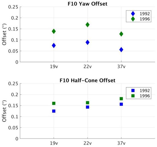
Figure 4.
Derived yaw (Top) and half-cone (Bottom) angle offsets for F10 19v, 22v, and 37v channels using observations from 1992 and 1996. The three channels and two years are averaged to give the final yaw and half-cone angle offsets.
Another significant difference between the SSMI(S) FCDR and the Level 1C datasets is that the pitch, roll, yaw, and half-cone angle offsets are fixed for each SSM/I sensor for the entire mission in the Level 1C, whereas the SSMI(S) FCDR dataset derived time-dependent pitch, roll, and yaw angle offsets [4]. There is some indication from Figure 4 that the F10 yaw offsets change between 1992 and 1996 by ~0.07°, as all three channels show this same difference. It should be noted that the DMSP F10 spacecraft is in a more eccentric orbit than the other five satellites carrying the SSM/I radiometers. This results in significantly larger altitude variations, and thus, variations in EIA of well over 1 degree for this instrument; however, the results indicate similar consistency in the derived roll, pitch, yaw and half-cone offsets over time, as for the other sensors. The other SSM/I sensors also exhibit small differences between the two years analyzed, though differences from the mean values are less than 0.05° for all cases. Also, differences or errors in the yaw offsets have no impact on the EIA, and thus the calibration, only on the calculated pixel latitude and longitude. Since the mount angles are not expected to change over time, the explanation for these time-dependent differences is likely due to changes in spacecraft attitude control or timing errors. Note that timing errors have the same impact as yaw offsets, and therefore, cannot be derived independently. While attitude errors might result in a slow change over time as the spacecraft orbit decays, it is also possible that changes could occur abruptly or more quickly than can be assessed using the coastline geolocation technique. As a result, we chose to use fixed values for the pitch, roll, yaw, and half-cone angle offsets and to consider these small time-dependent changes as a residual geolocation error, and with the exception of the yaw angle offsets, in the calculated pixel view angles.
Table 2 gives the updated pitch, roll, yaw, and half-cone angle offsets used for the Level 1C dataset. Figure 5 shows a comparison between the SSMI(S) FCDR and Level 1C geolocation for the F10 19v channel. The ascending minus descending gridded Tb are shown for the Australian coastline, divided into three scan position groups: left (scan positions 6 to 23), center (24 to 41) and right (42 to 59). While there are only minor differences between the SSMI(S) FCDR and Level 1C geolocation at the center of the scan, there are noticeable differences between the left and right sides of the scan. Since the SSMI(S) FCDR uses pre-launch values of the half-cone offset, the derived pitch has to account for offsets in the cone angle. Pitch and half-cone angle offsets have a similar impact on the geolocation at the center of the scan, but exhibit different behavior at the scan edges [15]. The Level 1C geolocation shows a similar pattern for the left, center, and right subsets of the scan, which confirms the accuracy of the pitch and roll values calculated from the cross-track scan Tb analysis.
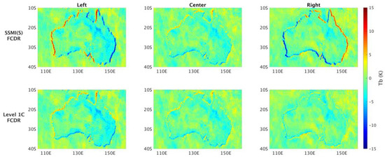
Figure 5.
F10 19v ascending minus descending gridded Tb for the SSMI(S) FCDR dataset (Top panels) versus the Level 1C dataset (Bottom panels). The SSMI scan is divided into left, center, and right subsets to show differences. The SSMI(S) FCDR dataset shows a significant change between the left and right sides of the scan indicating the attitude is incorrect, while the Level 1C dataset shows a consistent pattern across the scan.
3.1.3. SSM/I Level 1C Intercalibration
The SSM/I intercalibration for the Level 1C dataset uses GMI as the calibration reference, and applies a linear intercalibration adjustment based on differences over both cold ocean scenes and warm, unpolarized, vegetated land scenes. The dominant sources of calibration error are the antenna pattern spillover, emissive reflectors, and warm calibration target temperature errors, all of which can be corrected using a 2-point linear correction [12]. Analysis of on-orbit data from deep-space calibration maneuvers for GMI showed that errors in the spillover correction alone can easily result in scene-temperature dependent errors of several Kelvin, particularly for lower frequency channels with beam efficiency values of 95% or less [11]. Although there is no overlap between the SSM/I and GMI data records, the GMI calibration was linked back in time by first intercalibrating TMI using 1+ years of overlapping data [16], then using TMI to intercalibrate SSM/I on board F11, F13, F14, and F15, and finally linking the F11 calibration to F10 and then to F08. As mentioned previously, the original SSMI(S) FCDR was intercalibrated to the F13 SSM/I, which was chosen for its stability and the length of the available data record, not as an absolute calibration reference. The intercalibration was also based only on radiometrically cold ocean scenes, and thus, did not account for scene-dependent temperature differences in the calibration. While this was not that unreasonable for intercalibrating the SSM/I instruments given their similarity, it is unlikely to be the case relative to a high-quality calibration reference like GMI.
Intercalibration of the F11, F13, F14, and F15 SSM/I’s was done using multiple techniques, including double differences with the GMI-calibrated TMI Level 1C [7,12], a vicarious cold technique [18], and a vicarious warm-scene technique [19]. This is basically the same approach used by the XCAL team for the intercalibration of the GPM radiometer constellation, with multiple techniques over both cold and warm scenes providing a consistency check, as well as a measure of the residual uncertainties [12]. Details of the individual intercalibration techniques are left to the above references. For the F08 and F10 sensors, the intercalibration was somewhat more complicated, as a double difference approach with a well-calibrated instrument like TMI was not an option, and the results had to be daisy-chained between sensors to reference the results back to GMI. For F08, this meant comparing the calibration over a corresponding time period with F10, then to F11, and then to the GMI-calibration TMI Level 1C. As a result, the uncertainties for the F08 and F10 calibration are significantly larger, since the intercalibration estimates are subject to calibration uncertainties in the intermediate sensors. While the same vicarious cold [18] and warm [19] were used for these sensors, a single difference technique comparing simulated minus observed Tb for the sensor pairs was also used. This technique gives comparable results over ocean to the vicarious approach, but it does not work well over land, and thus, was not used for the warm scene calibration. Results from the vicarious warm-scene technique [19], however, show good agreement with double difference results versus TMI over vegetated land. As a result, both warm-scene techniques are used for the four SSM/I sensors overlapping the TMI data record, but only results from the vicarious warm technique are used for the F08 and F10 intercalibration.
The cold and warm scene calibration offsets for the six SSM/I instruments are given, along with the associated scene temperatures in Table 3. Given the similarity of the instruments, it is not surprising that the calibration offsets are similar, although there are differences between sensors. As with the prior Level 1C intercalibration by the XCAL team [12], the use of multiple techniques adds confidence to the validity of the results. For the GPM constellation sensors, the XCAL approach using multiple techniques found residual uncertainties in the intercalibration offsets within 0.5 K over cold scenes (ocean) and within 1.0 K over warm scenes (vegetated land) [12]. Results from the various techniques for the SSM/I sensors discussed here are consistent with those results. Calibration errors relative to the GMI reference standard, however, are significantly larger for the older SSM/I sensors in particular due to uncertainties in the intercalibration of the intermediate sensors, as well as potential calibration drifts that have not been fully corrected for. Given the lack of a long-term calibration reference, the best guidance for users is to consider small climate trends or changes in retrieved geophysical variables with skepticism, particularly for the pre-TRMM data record.
Table 3.
Intercalibration offsets in Kelvin for the six SSM/I sensors for both cold and warm scenes. Corresponding scene temperature values are indicated in parentheses.
4. Discussion
The data record from conical-scanning window channel microwave radiometers shown in Figure 2 provides nearly continuous global coverage over a 30+ year period. While data from this constellation of operational and research satellites is of significant value for a wide array of applications, the instruments were not designed for such collective applications. Sensor differences, data formats, a variety of calibration issues, and inconsistencies in the calibration between sensors, even “identical” copies of instruments such as SSM/I, make it both difficult and risky to develop and apply retrieval algorithms to the available sensors. The SSMI(S) and Level 1C FCDRs described here are attempts to correct for known calibration errors, and to intercalibrate data from the various sensors to a specified calibration reference sensor. The FCDR data, however, does not attempt to adjust or “correct” for sensor differences such as frequency, polarization, bandwidth, and view angle. For example, the SSM/I 22.235 GHz channel does not respond the same to geophysical parameters within a given scene as the GMI 23.8 GHz channel. Any attempt to adjust for these differences must take into account the properties impacting emitted radiation at this frequency, including water vapor, cloud water, surface emissivity, surface wind speed, etc.
Accounting for expected differences due to frequency, view angle, etc., therefore, is left to the geophysical retrieval algorithms. As described above, significant efforts have been made to provide accurate view angle or EIA for each pixel in the FCDR datasets. Small changes in EIA can have a significant impact on the Tb, especially over water, due to changes in the surface emissivity. Additionally, changes in view angle change the slant path, and thus the column of atmosphere being sensed. Over water, changes in surface emissivity and the slant path corresponding to a change in the view angle are additive for the vertically-polarized channels, but mostly cancel out for the horizontally-polarized channels. This is the reason why the roll and pitch offsets are derived using only the low-frequency v-pol channels. For relatively small changes in the EIA, changes in Tb, as well as the relative change in the polarization difference can have a significant impact on retrieval algorithms, particularly for retrieving parameters such as ocean surface winds. The DMSP instruments in particular are not in controlled orbits, meaning that the orbits decay over time. This changes not only the local observing time, and thus the diurnal sampling, but also the mean view angle due to the change in altitude. While the impact of changes in EIA are larger for F10 due to the eccentricity of the orbit, changes in EIA both over an orbit and due to orbit decay are significant for all of the SSM/I’s. If geophysical retrieval algorithms do not properly account for these view angle changes, it can result in false trends in the resulting climate data records.
5. Conclusions
Global observations from high-quality satellite passive microwave imagers extending over 30+ years provide a valuable resource for long-term monitoring of a wide range of atmospheric and surface parameters. Inconsistencies in the calibration and characterization of these data between sensors, however, limit their usefulness for such applications. To address these inconsistencies, an initial effort focused on producing an intercalibrated FCDR from the series of 10 SSM/I and SSMIS radiometers on board the DMSP satellites. This SSMI(S) FCDR incorporates quality control of the data, corrections for cross-track biases, view angle, and geolocation errors, emissive reflector issues, solar and lunar intrusions into the warm load, antenna pattern spillover effects, and intercalibration of the brightness temperatures between instruments. Although the six SSM/I and four SSMIS instruments are “identical” copies, there are significant differences between the sensors. Corrections were developed and applied to make the FCDR brightness temperatures physically consistent; however, physical differences remain that must be accounted for by retrieval algorithms. These include changes in channel frequencies between SSM/I and SSMIS and both short-term view angle variations, particularly for the more eccentric F10 orbit, as well as long-term variations due to the decay of the orbits. The SSMI(S) FCDR data is available as orbitized granules in NetCDF4 at the original sampling and spatial resolution from both NOAA (https://www.ncdc.noaa.gov/cdr/fundamental/ssmis-brightness-temperature-csu) and from Colorado State University (http://rain.atmos.colostate.edu/FCDR), with an interim climate data record (ICDR) updated in near real-time and updates to the FCDR done once per year.
A subsequent effort to intercalibrate the available constellation of microwave radiometers for the GPM precipitation mission led to the development of a Level 1C FCDR dataset. These data are available from the NASA Precipitation Processing System (https://pmm.nasa.gov/data-access/downloads/gpm). As with the SSMI(S) FCDR, the Level 1C data have corrections applied to make the Tb physically consistent, but differences due to variations in channel frequencies, polarization, spectral band width, and view angle remain. Originally developed for the GPM constellation sensors starting with the launch of the GPM core satellite in February of 2014, it has since been extended back to SSM/I on board DMSP F08 in July of 1987. The Level 1C dataset has data from several additional conical-scanning window channel radiometers including TRMM TMI, GPM GMI, EOS-AQUA AMSR-E, and GCOM-W1 AMSR2. It uses the GPM GMI instrument as a calibration reference, which, as a result of the design and based on post-launch calibration analysis, provides an excellent absolute calibration reference. Several updates have been made to the corrections applied to the SSM/I Level 1C data from the original SSMI(S) FCDR, including the cross-scan bias and geolocation corrections and a scene-temperature dependent intercalibration adjustment. Both the SSMI(S) FCDR and the Level 1C FCDR include the view angle for each pixel along with other relevant sensor information needed to produce consistent climate data records of retrieved geophysical products.
Author Contributions
Conceptualization, W.B. and C.D.K.; Methodology, Software Validation, Formal Analysis, and Investigation, W.B., R.K. and D.S.M.; Writing-Original Draft Preparation, Writing-Review & Editing, and Visualization, W.B. and R.K.; Data Curation, W.B.; Project Administration, W.B. and C.D.K.; Funding Acquisition and Resources, W.B., C.D.K., and D.S.M.
Funding
This research was funded by NASA grant numbers NNX16AE23G and NNX16AE38G.
Acknowledgments
Support for this work was provided by the NASA Precipitation Processing System at Goddard Space Flight Center.
Conflicts of Interest
The authors declare no conflict of interest. The funding sponsors had no role in the design of the study; in the collection, analyses, or interpretation of data; in the writing of the manuscript, and in the decision to publish the results.
References
- National Research Council. Climate Data Records from Environmental Satellites; Interim Report; The National Academies Press: Washinton, DC, USA, 2004. [Google Scholar] [CrossRef]
- Berg, W.K.; Rodriguez-Alvarez, N. SSM/I and SSMIS Quality Control; Technical Report; Colorado State University: Fort Collins, CO, USA, 2013. [Google Scholar]
- Berg, W.; Sapiano, M.R.P. Corrections and APC for SSMIS; Technical Report; Colorado State University: Fort Collins, CO, USA, 2013. [Google Scholar]
- Berg, W.; Sapiano, M.R.P.; Horsman, J.; Kummerow, C. Improved geolocation and Earth incidence angle information for a fundamental climate data record of the SSM/I sensors. Trans. Geosci. Remote Sens. 2013, 51, 1504–1513. [Google Scholar] [CrossRef]
- Sapiano, M.R.P.; Berg, W.K. Estimation of Satellite Attitude for SSM/I and SSMIS Geolocation; Technical Report; Colorado State University: Fort Collins, CO, USA, 2012. [Google Scholar]
- Sapiano, M.R.P.; Bilanow, S.; Berg, W. SSM/I and SSMIS Stewardship Code Geolocation Algorithm Theoretical Basis; Technical Report; Colorado State University: Fort Collins, CO, USA, 2010. [Google Scholar]
- Sapiano, M.R.P.; Berg, W.; McKague, D.; Kummerow, C. Towards an intercalibrated fundamental climate data record of the SSM/I sensors. Trans. Geosci. Remote Sens. 2013, 51, 1492–1503. [Google Scholar] [CrossRef]
- Sapiano, M.R.P.; Berg, W. Intercalibration of SSM/I and SSMIS for the CSU FCDR; Technical Report; Colorado State University: Fort Collins, CO, USA, 2013. [Google Scholar]
- Hou, A.Y.; Kakar, R.K.; Neeck, S.; Azarbarzin, A.A.; Kummerow, C.D.; Kojima, M.; Oki, R.; Nakamura, K.; Iguchi, T. The Global Precipitation Measurement Mission. Bull. Am. Meteorol. Soc. 2014, 95, 701–722. [Google Scholar] [CrossRef]
- Skofronick-Jackson, G.; Petersen, W.A.; Berg, W.; Kidd, C.; Stocker, E.F.; Kirschbaum, D.B.; Kakar, R.; Braun, S.A.; Huffman, G.J.; Iguchi, T.; et al. The Global Precipitation Measurement (GPM) mission for science and society. Bull. Am. Meteorol. Soc. 2017, 98, 1679–1696. [Google Scholar] [CrossRef]
- Wentz, F.; Draper, D. On-orbit absolute calibration of the Global Precipitation Mission microwave imager. J. Atmos. Ocean. Technol. 2016, 33, 1393–1412. [Google Scholar] [CrossRef]
- Berg, W.; Bilanow, S.; Chen, R.; Datta, S.; Draper, D.; Ebrahimi, H.; Farrar, S.; Jones, W.L.; Kroodsma, R.; McKagu, D.; et al. Intercalibration of the GPM Radiometer Constellation. J. Atmos. Ocean. Technol. 2016, 33, 2639–2654. [Google Scholar] [CrossRef]
- Alquaied, F.; Chen, R.; Jonesm, W.L. Hot load temperature correction for TRMM microwave imager in the legacy brightness temperature temperature. IEEE J. Sel. Top. Appl. Earth Observ. 2018, 99, 1–9. [Google Scholar] [CrossRef]
- Alquaied, F.; Chen, R.; Jones, W.L. Emissive reflector correction in the legacy version 1B11 V8 (GPM05) brightness temperature of the TRMM microwave imager. IEEE J. Sel. Top. Appl. Earth Observ. 2018, 11, 1905–1912. [Google Scholar] [CrossRef]
- Kroodsma, R.; Bilanow, S.; McKague, D.S. TRMM Microwave Imager (TMI) alignment and along-scan bias corrections. J. Atmos. Ocean. Technol. 2018, 35. [Google Scholar] [CrossRef]
- Berg, W. Towards developing a long-term high-quality intercalibrated TRMM/GPM radiometer dataset. In Proceedings of the 2017 IEEE International Geoscience and Remote Sensing Symposium (IGARSS), Fort Worth, TX, USA, 23–28 July 2017; pp. 248–250. [Google Scholar]
- Colton, M.C.; Poe, G.A. Intersensor calibration of DMSP SSM/I’s: F-8 to F-14, 1987–1997. IEEE Trans. Geosci. Remote Sens. 1999, 37, 418–439. [Google Scholar] [CrossRef]
- Kroodsma, R.A.; McKague, D.S.; Ruf, C.S. Vicarious cold calibration for conical scanning microwave imagers. IEEE Trans. Geosci. Rem. Sens. 2016, 55, 816–827. [Google Scholar] [CrossRef]
- Yang, J.X.; McKague, D.S.; Ruf, C.S. Boreal, temperate, and tropical forests as vicarious calibration sites for spaceborne microwave radiometry. IEEE Trans. Geosci. Rem. Sens. 2016, 54, 1035–1051. [Google Scholar] [CrossRef]


© 2018 by the authors. Licensee MDPI, Basel, Switzerland. This article is an open access article distributed under the terms and conditions of the Creative Commons Attribution (CC BY) license (http://creativecommons.org/licenses/by/4.0/).