An Operational Workflow of Deciduous-Dominated Forest Species Classification: Crown Delineation, Gap Elimination, and Object-Based Classification †


Abstract
1. Introduction
2. Study Area and Datasets
2.1. Study Area
2.2. Multi-Seasonal WorldView-2 and WorldView-3 Images
2.3. Field Data for Training and Test Classifications
3. Methods
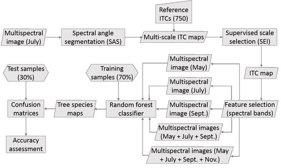
3.1. Overview
3.2. Individual Tree Crown Delineation
3.3. Object-Based Species Classification
4. Results
4.1. ITC Delineation
4.2. Individual Tree-Based Species Classification
5. Discussion
Workflow of Individual Tree-Based Species Classification
6. Conclusions and Future Work
Author Contributions
Funding
Acknowledgments
Conflicts of Interest
References
- Breidenbach, J.; Næsset, E.; Lien, V.; Gobakken, T.; Solberg, S. Prediction of species specific forest inventory attributes using a nonparametric semi-individual tree crown approach based on fused airborne laser scanning and multispectral data. Remote Sens. Environ. 2010, 114, 911–924. [Google Scholar] [CrossRef]
- Haara, A.; Haarala, M. Tree species classification using semi-automatic delineation of trees on aerial images. Scand. J. For. Res. 2002, 17, 556–565. [Google Scholar] [CrossRef]
- Ørka, H.O.; Gobakken, T.; Næsset, E.; Ene, L.; Lien, V. Simultaneously acquired airborne laser scanning and multispectral imagery for individual tree species identification. Can. J. Remote Sens. 2012, 38, 125–138. [Google Scholar] [CrossRef]
- Waser, L.; Ginzler, C.; Kuechler, M.; Baltsavias, E.; Hurni, L. Semi-automatic classification of tree species in different forest ecosystems by spectral and geometric variables derived from Airborne Digital Sensor (ADS40) and RC30 data. Remote Sens. Environ. 2011, 115, 76–85. [Google Scholar] [CrossRef]
- Dalponte, M.; Ørka, H.O.; Ene, L.T.; Gobakken, T.; Næsset, E. Tree crown delineation and tree species classification in boreal forests using hyperspectral and ALS data. Remote Sens. Environ. 2014, 140, 306–317. [Google Scholar] [CrossRef]
- Heinzel, J.; Koch, B. Investigating multiple data sources for tree species classification in temperate forest and use for single tree delineation. Int. J. Appl. Earth Obs. Geoinf. 2012, 18, 101–110. [Google Scholar] [CrossRef]
- Ke, Y.; Quackenbush, L.J. A review of methods for automatic individual tree-crown detection and delineation from passive remote sensing. Int. J. Remote Sens. 2011, 32, 4725–4747. [Google Scholar] [CrossRef]
- Yang, J.; Jones, T.; Caspersen, J.; He, Y. Object-based canopy gap segmentation and classification: Quantifying the pros and cons of integrating optical and LiDAR data. Remote Sens. 2015, 7, 15917–15932. [Google Scholar] [CrossRef]
- Yang, J.; He, Y.; Caspersen, J.P.; Jones, T.A. Delineating individual tree crowns in an uneven-aged, mixed broadleaf forest using multispectral watershed segmentation and multiscale fitting. IEEE J. Sel. Top. Appl. Earth Obs. Remote Sens. 2017, 10, 1390–1401. [Google Scholar] [CrossRef]
- Jing, L.; Hu, B.; Noland, T.; Li, J. An individual tree crown delineation method based on multi-scale segmentation of imagery. ISPRS J. Photogramm. Remote Sens. 2012, 70, 88–98. [Google Scholar] [CrossRef]
- Pu, R.; Landry, S. A comparative analysis of high spatial resolution IKONOS and WorldView-2 imagery for mapping urban tree species. Remote Sens. Environ. 2012, 124, 516–533. [Google Scholar] [CrossRef]
- Yu, Q.; Gong, P.; Clinton, N.; Biging, G.; Kelly, M.; Schirokauer, D. Object-based detailed vegetation classification with airborne high spatial resolution remote sensing imagery. Photogramm. Eng. Remote Sens. 2006, 72, 799–811. [Google Scholar] [CrossRef]
- Clark, M.L.; Roberts, D.A.; Clark, D.B. Hyperspectral discrimination of tropical rain forest tree species at leaf to crown scales. Remote Sens. Environ. 2005, 96, 375–398. [Google Scholar] [CrossRef]
- Dalponte, M.; Orka, H.O.; Gobakken, T.; Gianelle, D.; Næsset, E. Tree species classification in boreal forests with hyperspectral data. IEEE Trans. Geosci. Remote Sens. 2013, 51, 2632–2645. [Google Scholar] [CrossRef]
- Greenberg, J.A.; Dobrowski, S.Z.; Ramirez, C.M.; Tuil, J.L.; Ustin, S.L. A bottom-up approach to vegetation mapping of the Lake Tahoe Basin using hyperspatial image analysis. Photogramm. Eng. Remote Sens. 2006, 72, 581–589. [Google Scholar] [CrossRef]
- Immitzer, M.; Atzberger, C.; Koukal, T. Tree species classification with random forest using very high spatial resolution 8-band WorldView-2 satellite data. Remote Sens. 2012, 4, 2661–2693. [Google Scholar] [CrossRef]
- Leckie, D.G.; Tinis, S.; Nelson, T.; Burnett, C.; Gougeon, F.A.; Cloney, E.; Paradine, D. Issues in species classification of trees in old growth conifer stands. Can. J. Remote Sens. 2005, 31, 175–190. [Google Scholar] [CrossRef]
- Leckie, D.G.; Walsworth, N.; Gougeon, F.A. Identifying tree crown delineation shapes and need for remediation on high resolution imagery using an evidence based approach. ISPRS J. Photogramm. Remote Sens. 2016, 114, 206–227. [Google Scholar] [CrossRef]
- Leckie, D.G.; Walsworth, N.; Gougeon, F.A.; Gray, S.; Johnson, D.; Johnson, L.; Oddleifson, K.; Plotsky, D.; Rogers, V. Automated individual tree isolation on high-resolution imagery: Possible methods for breaking isolations involving multiple trees. IEEE J. Sel. Top. Appl. Earth Obs. Remote Sens. 2016, 9, 3229–3248. [Google Scholar] [CrossRef]
- Breiman, L. Random forests. Mach. Learn. 2001, 45, 5–32. [Google Scholar] [CrossRef]
- Dalponte, M.; Bruzzone, L.; Gianelle, D. Tree species classification in the Southern Alps based on the fusion of very high geometrical resolution multispectral/hyperspectral images and LiDAR data. Remote Sens. Environ. 2012, 123, 258–270. [Google Scholar] [CrossRef]
- Korpela, I.; Ørka, H.O.; Maltamo, M.; Tokola, T.; Hyyppä, J. Tree species classification using airborne LiDAR—Effects of stand and tree parameters, downsizing of training set, intensity normalization, and sensor type. Silva. Fenn. 2010, 44, 319–339. [Google Scholar] [CrossRef]
- Ørka, H.O.; Næsset, E.; Bollandsås, O.M. Effects of different sensors and leaf-on and leaf-off canopy conditions on echo distributions and individual tree properties derived from airborne laser scanning. Remote Sens. Environ. 2010, 114, 1445–1461. [Google Scholar] [CrossRef]
- Cho, M.A.; Debba, P.; Mutanga, O.; Dudeni-Tlhone, N.; Magadla, T.; Khuluse, S.A. Potential utility of the spectral red-edge region of SumbandilaSat imagery for assessing indigenous forest structure and health. Int. J. Appl. Earth Obs. Geoinf. 2012, 16, 85–93. [Google Scholar] [CrossRef]
- Madonsela, S.; Cho, M.A.; Mathieu, R.; Mutanga, O.; Ramoelo, A.; Kaszta, Ż.; Kerchove, R.V.D.; Wolff, E. Multi-phenology WorldView-2 imagery improves remote sensing of savannah tree species. Int. J. Appl. Earth Obs. Geoinf. 2017, 58, 65–73. [Google Scholar] [CrossRef]
- Cho, M.; Naidoo, L.; Mathieu, R.; Asner, G. Mapping savanna tree species using Carnegie Airborne Observatory hyperspectral data resampled to WorldView-2 multispectral configuration. In Proceedings of the 34th International Symposium on Remote Sensing of Environment, Sydney, Australia, 10–15 April 2011. [Google Scholar]
- Latif, Z.A.; Zamri, I.; Omar, H. Determination of tree species using Worldview-2 data. In Proceedings of the IEEE 8th International Colloquium on Signal Processing and Its Applications (CSPA), Malacca, Malaysia, 23–25 March 2012. [Google Scholar]
- Key, T.; Warner, T.A.; McGraw, J.B.; Fajvan, M.A. A comparison of multispectral and multitemporal information in high spatial resolution imagery for classification of individual tree species in a temperate hardwood forest. Remote Sens. Environ. 2001, 75, 100–112. [Google Scholar] [CrossRef]
- Hill, R.; Wilson, A.; George, M.; Hinsley, S. Mapping tree species in temperate deciduous woodland using time-series multi-spectral data. Appl. Veg. Sci. 2010, 13, 86–99. [Google Scholar] [CrossRef]
- Pipkins, K.; Förster, M.; Clasen, A.; Schmidt, T.; Kleinschmit, B. A comparison of feature selection methods for multitemporal tree species classification. In Proceedings of the Earth Resources and Environmental Remote Sensing/GIS Applications V. International Society for Optics and Photonics, Amsterdam, The Netherlands, 23–25 September 2014. [Google Scholar]
- Pu, R.; Landry, S.; Yu, Q. Assessing the Potential of Multi-Seasonal High Resolution Pléiades Satellite Pleiades Imagery for Mapping Urban Tree Species. Int. J. Appl. Earth Obs. Geoinf. 2018, 71, 144–158. [Google Scholar] [CrossRef]
- Hossain, S.M.Y.; Caspersen, J.P. In-situ measurement of twig dieback and regrowth in mature Acer saccharum trees. For. Ecol. Manag. 2012, 270, 183–188. [Google Scholar] [CrossRef]
- Laben, C.A.; Brower, B.V. Process for Enhancing the Spatial Resolution of Multispectral Imagery Using Pan-Sharpening. U.S. Patent 6,011,875, 4 January 2000. [Google Scholar]
- Nikolakopoulos, K.; Oikonomidis, D. Quality assessment of ten fusion techniques applied on Worldview-2. Eur. J. Remote Sens. 2015, 48, 141–167. [Google Scholar] [CrossRef]
- Delisle, G.P.; Woodward, M.P.; Titus, S.J.; Johnson, A.F. Sample size and variability of fuel weight estimates in natural stands of lodgepole pine. Can. J. Res. 1988, 18, 649–652. [Google Scholar] [CrossRef]
- Yang, J.; He, Y.; Caspersen, J. A multi-band watershed segmentation method for individual tree crown delineation from high resolution multispectral aerial image. In Proceedings of the 2014 IEEE International Geoscience and Remote Sensing Symposium (IGARSS), Quebec City, QC, Canada, 13–18 July 2014. [Google Scholar]
- Yang, J.; He, Y.; Caspersen, J.; Jones, T. A discrepancy measure for segmentation evaluation from the perspective of object recognition. ISPRS J. Photogramm. Remote Sens. 2015, 101, 186–192. [Google Scholar] [CrossRef]
- Vincent, L.; Soille, P. Watersheds in digital spaces: An efficient algorithm based on immersion simulations. IEEE Trans. Pattern Anal. Mach. Intell. 1991, 13, 583–598. [Google Scholar] [CrossRef]
- Conrad, O.; Bechtel, B.; Bock, M.; Dietrich, H.; Fischer, E.; Gerlitz, L.; Wehberg, J.; Wichmann, V.; Böhner, J. System for Automated Geoscientific Analyses (SAGA) v. 2.1. 4. Geosci. Model. Dev. Discuss. 2015, 8, 2271–2312. [Google Scholar] [CrossRef]
- Hastie, T.; Tibshirani, R.; Friedman, J. The Elements of Statistical Learning; Springer: New York, NY, USA, 2001; Volume 1. [Google Scholar]
- Immitzer, M.; Böck, S.; Einzmann, K.; Vuolo, F.; Pinnel, N.; Wallner, A.; Atzberger, C. Fractional cover mapping of spruce and pine at 1 ha resolution combining very high and medium spatial resolution satellite imagery. Remote Sens. Environ. 2018, 204, 690–703. [Google Scholar] [CrossRef]
- Hossain, S.M.Y.; Caspersen, J.P.; Thomas, S.C. Reproductive costs in Acer saccharum: Exploring size-dependent relations between seed production and branch extension. Trees 2017, 31, 1179–1188. [Google Scholar] [CrossRef]
- Somers, B.; Asner, G.P. Tree species mapping in tropical forests using multi-temporal imaging spectroscopy: Wavelength adaptive spectral mixture analysis. Int. J. Appl. Earth Obs. Geoinf. 2014, 31, 57–66. [Google Scholar] [CrossRef]
- Wolter, P.T.; Mladenoff, D.J.; Host, G.E.; Crow, T.R. Improved forest classification in the Northern Lake States using multi-temporal Landsat imagery. Photogramm. Eng. Remote Sens. 1995, 61, 1129–1143. [Google Scholar]
- Zhang, W.; Quackenbush, L.J.; Im, J.; Zhang, L. Indicators for separating undesirable and well-delineated tree crowns in high spatial resolution images. Int. J. Remote Sens. 2012, 33, 5451–5472. [Google Scholar] [CrossRef]
- Guo, Y.; Liu, Y.; Georgiou, T.; Lew, M.S. A review of semantic segmentation using deep neural networks. Int. J. Multimed. Inf. Retr. 2018, 7, 87–93. [Google Scholar] [CrossRef]
- Weinstein, B.G.; Marconi, S.; Bohlman, S.; Zare, A.; White, E. Individual Tree-Crown Detection in RGB Imagery Using Semi-Supervised Deep Learning Neural Networks. Remote Sens. 2019, 11, 1309. [Google Scholar] [CrossRef]


| Species | Mh | Mr | Be | By | He | Or | Bf | Total |
|---|---|---|---|---|---|---|---|---|
| Transect 1 | 94 | 20 | 31 | 29 | 30 | 0 | 16 | 220 |
| Transect 2 | 81 | 42 | 24 | 21 | 33 | 26 | 7 | 234 |
| Transect 3 | 101 | 2 | 39 | 39 | 32 | 0 | 5 | 218 |
| Total | 276 | 64 | 94 | 89 | 95 | 26 | 28 | 672 |
| Independent Use of Late-spring Image | Independent Use of Mid-summer Image | ||||||||||||||
| Mh | Mr | Be | By | He | Or | Bf | Mh | Mr | Be | By | He | Or | Bf | ||
| Mh | 36 | 2 | 4 | 4 | 1 | 2 | 0 | Mh | 31 | 2 | 3 | 2 | 1 | 1 | 0 |
| Mr | 2 | 4 | 1 | 3 | 1 | 0 | 1 | Mr | 12 | 7 | 1 | 6 | 6 | 2 | 1 |
| Be | 9 | 3 | 11 | 1 | 4 | 0 | 1 | Be | 8 | 2 | 11 | 2 | 2 | 0 | 1 |
| By | 12 | 5 | 3 | 7 | 6 | 1 | 0 | By | 10 | 0 | 3 | 7 | 4 | 0 | 1 |
| He | 3 | 1 | 1 | 4 | 11 | 0 | 0 | He | 2 | 1 | 4 | 2 | 10 | 1 | 0 |
| Or | 3 | 0 | 1 | 0 | 0 | 3 | 0 | Or | 4 | 1 | 0 | 0 | 1 | 2 | 0 |
| Bf | 4 | 0 | 1 | 3 | 4 | 0 | 4 | Bf | 2 | 2 | 1 | 4 | 2 | 0 | 3 |
| PA | 0.52 | 0.27 | 0.50 | 0.32 | 0.41 | 0.50 | 0.67 | PA | 0.45 | 0.47 | 0.48 | 0.30 | 0.38 | 0.33 | 0.50 |
| UA | 0.73 | 0.33 | 0.38 | 0.21 | 0.55 | 0.43 | 0.25 | UA | 0.78 | 0.20 | 0.42 | 0.28 | 0.50 | 0.25 | 0.21 |
| OA | 0.46 | KIA | 0.31 | OA | 0.42 | KIA | 0.29 | ||||||||
| Independent Use of Early-fall Image | Combined Use of Late-spring, Mid-summer, Early-fall Images | ||||||||||||||
| Mh | Mr | Be | By | He | Or | Bf | Mh | Mr | Be | By | He | Or | Bf | ||
| Mh | 16 | 2 | 4 | 3 | 5 | 0 | 0 | Mh | 45 | 0 | 1 | 1 | 0 | 0 | 0 |
| Mr | 12 | 6 | 3 | 6 | 1 | 0 | 0 | Mr | 6 | 15 | 0 | 2 | 1 | 0 | 0 |
| Be | 5 | 2 | 6 | 0 | 1 | 1 | 0 | Be | 4 | 0 | 21 | 0 | 3 | 0 | 0 |
| By | 4 | 0 | 4 | 7 | 2 | 0 | 0 | By | 8 | 0 | 0 | 18 | 0 | 0 | 0 |
| He | 13 | 2 | 3 | 1 | 13 | 1 | 0 | He | 0 | 0 | 1 | 0 | 21 | 0 | 0 |
| Or | 7 | 0 | 1 | 1 | 3 | 3 | 1 | Or | 3 | 0 | 0 | 0 | 1 | 6 | 0 |
| Bf | 5 | 0 | 1 | 3 | 0 | 1 | 2 | Bf | 3 | 0 | 0 | 2 | 0 | 0 | 6 |
| PA | 0.26 | 0.50 | 0.27 | 0.33 | 0.52 | 0.50 | 0.67 | PA | 0.65 | 1.00 | 0.91 | 0.78 | 0.81 | 1.00 | 1.00 |
| UA | 0.53 | 0.21 | 0.40 | 0.41 | 0.39 | 0.19 | 0.17 | UA | 0.96 | 0.63 | 0.75 | 0.69 | 0.95 | 0.60 | 0.55 |
| OA | 0.35 | KIA | 0.19 | OA | 0.79 | KIA | 0.73 | ||||||||
| Integration of All Four Scenes | |||||||||||||||
| Mh | Mr | Be | By | He | Or | Bf | |||||||||
| Mh | 48 | 2 | 6 | 3 | 0 | 3 | 0 | ||||||||
| Mr | 6 | 8 | 2 | 1 | 8 | 0 | 1 | ||||||||
| Be | 4 | 1 | 9 | 1 | 2 | 0 | 1 | ||||||||
| By | 7 | 2 | 4 | 6 | 2 | 0 | 0 | ||||||||
| He | 2 | 1 | 2 | 8 | 12 | 1 | 0 | ||||||||
| Or | 1 | 1 | 0 | 0 | 1 | 2 | 0 | ||||||||
| Bf | 1 | 0 | 0 | 4 | 1 | 0 | 4 | ||||||||
| PA | 0.70 | 0.53 | 0.39 | 0.26 | 0.46 | 0.33 | 0.67 | ||||||||
| UA | 0.77 | 0.31 | 0.50 | 0.29 | 0.46 | 0.40 | 0.40 | ||||||||
| OA | 0.53 | KIA | 0.39 | ||||||||||||
| Using Eight Bands of Multispectral WorldView Images | Using Four Traditional Bands of Multispectral WorldView Images | ||||||||||||||
|---|---|---|---|---|---|---|---|---|---|---|---|---|---|---|---|
| Mh | Mr | Be | By | He | Or | Bf | Mh | Mr | Be | By | He | Or | Bf | ||
| Mh | 45 | 0 | 1 | 1 | 0 | 0 | 0 | Mh | 49 | 3 | 5 | 4 | 2 | 2 | 0 |
| Mr | 6 | 15 | 0 | 2 | 1 | 0 | 0 | Mr | 5 | 6 | 0 | 2 | 3 | 0 | 1 |
| Be | 4 | 0 | 21 | 0 | 3 | 0 | 0 | Be | 5 | 2 | 9 | 2 | 3 | 1 | 1 |
| By | 8 | 0 | 0 | 18 | 0 | 0 | 0 | By | 3 | 1 | 4 | 9 | 4 | 0 | 0 |
| He | 0 | 0 | 1 | 0 | 21 | 0 | 0 | He | 1 | 1 | 2 | 3 | 9 | 0 | 0 |
| Or | 3 | 0 | 0 | 0 | 1 | 6 | 0 | Or | 4 | 2 | 1 | 0 | 2 | 3 | 0 |
| Bf | 3 | 0 | 0 | 2 | 0 | 0 | 6 | Bf | 2 | 0 | 2 | 3 | 3 | 0 | 4 |
| PA | 0.65 | 1.00 | 0.91 | 0.78 | 0.81 | 1.00 | 1.00 | PA | 0.71 | 0.40 | 0.39 | 0.39 | 0.35 | 0.50 | 0.67 |
| UA | 0.96 | 0.63 | 0.75 | 0.69 | 0.95 | 0.60 | 0.55 | UA | 0.75 | 0.35 | 0.39 | 0.43 | 0.56 | 0.25 | 0.29 |
| OA | 0.79 | KIA | 0.73 | OA | 0.53 | KIA | 0.39 | ||||||||
© 2019 by the authors. Licensee MDPI, Basel, Switzerland. This article is an open access article distributed under the terms and conditions of the Creative Commons Attribution (CC BY) license (http://creativecommons.org/licenses/by/4.0/).
Share and Cite
He, Y.; Yang, J.; Caspersen, J.; Jones, T. An Operational Workflow of Deciduous-Dominated Forest Species Classification: Crown Delineation, Gap Elimination, and Object-Based Classification. Remote Sens. 2019, 11, 2078. https://doi.org/10.3390/rs11182078
He Y, Yang J, Caspersen J, Jones T. An Operational Workflow of Deciduous-Dominated Forest Species Classification: Crown Delineation, Gap Elimination, and Object-Based Classification. Remote Sensing. 2019; 11(18):2078. https://doi.org/10.3390/rs11182078
Chicago/Turabian StyleHe, Yuhong, Jian Yang, John Caspersen, and Trevor Jones. 2019. "An Operational Workflow of Deciduous-Dominated Forest Species Classification: Crown Delineation, Gap Elimination, and Object-Based Classification" Remote Sensing 11, no. 18: 2078. https://doi.org/10.3390/rs11182078
APA StyleHe, Y., Yang, J., Caspersen, J., & Jones, T. (2019). An Operational Workflow of Deciduous-Dominated Forest Species Classification: Crown Delineation, Gap Elimination, and Object-Based Classification. Remote Sensing, 11(18), 2078. https://doi.org/10.3390/rs11182078