Article

Methodology for Processing of 3D Multibeam Sonar Big Data for Comparative Navigation

by
Andrzej Stateczny
1,*,
Wioleta Błaszczak-Bąk
2,
Anna Sobieraj-Żłobińska
1,
Weronika Motyl
3 and
Marta Wisniewska
3
1
Department of Geodesy, Faculty of Civil and Environmental Engineering, Gdansk University of Technology, Narutowicza 11-12, 80-233 Gdansk, Poland
2
Institute of Geodesy, Faculty of Geodesy, Geospatial and Civil Engineering, University of Warmia and Mazury in Olsztyn, Oczapowskiego 2, 10-719 Olsztyn, Poland
3
Marine Technology Ltd., Roszczynialskiego 4/6, 81-521 Gdynia, Poland
*
Author to whom correspondence should be addressed.
Remote Sens. 2019, 11(19), 2245; https://doi.org/10.3390/rs11192245
Submission received: 30 July 2019 / Revised: 23 September 2019 / Accepted: 24 September 2019 / Published: 26 September 2019
(This article belongs to the Special Issue Radar and Sonar Imaging and Processing)

Abstract

:
Autonomous navigation is an important task for unmanned vehicles operating both on the surface and underwater. A sophisticated solution for autonomous non-global navigational satellite system navigation is comparative (terrain reference) navigation. We present a method for fast processing of 3D multibeam sonar data to make depth area comparable with depth areas from bathymetric electronic navigational charts as source maps during comparative navigation. Recording the bottom of a channel, river, or lake with a 3D multibeam sonar data produces a large number of measuring points. A big dataset from 3D multibeam sonar is reduced in steps in almost real time. Usually, the whole data set from the results of a multibeam echo sounder results are processed. In this work, new methodology for processing of 3D multibeam sonar big data is proposed. This new method is based on the stepwise processing of the dataset with 3D models and isoline maps generation. For faster products generation we used the optimum dataset method which has been modified for the purposes of bathymetric data processing. The approach enables detailed examination of the bottom of bodies of water and makes it possible to capture major changes. In addition, the method can detect objects on the bottom, which should be eliminated during the construction of the 3D model. We create and combine partial 3D models based on reduced sets to inspect the bottom of water reservoirs in detail. Analyses were conducted for original and reduced datasets. For both cases, 3D models were generated in variants with and without overlays between them. Tests show, that models generated from reduced dataset are more useful, due to the fact, that there are significant elements of the measured area that become much more visible, and they can be used in comparative navigation. In fragmentary processing of the data, the aspect of present or lack of the overlay between generated models did not relevantly influence the accuracy of its height, however, the time of models generation was shorter for variants without overlay.

1. Introduction

Unmanned underwater vehicles, also known as underwater robots, have developed rapidly over the past few years. These systems supersede previously used methods of the underwater exploration of Earth, such as, e.g., hydrographic measuring units with human crew. The trend in unmanned systems development is toward the execution of underwater tasks, including hydrographical surveys, near the bottom by underwater robots, such as remotely operated vehicles remotely controlled by an operator and autonomous underwater vehicles (AUVs) operated without operator input. Underwater positioning methods are not keeping pace with the fast development of AUVs and measurement tools. The main global navigational satellite system (GNSS) positioning method for submersible vehicles is limited to situations where the submersible vehicle can raise an antenna above the surface of the water. However, some AUVs need the more independent method of comparative (terrain) navigation via digital terrain models (DTMs) [1,2,3,4,5,6,7].
New methods of spatial data measurement using interferometric multibeam echosounders (MBES), high-frequency side scan sonar, and integrated MBES with sonars require new data processing methods. These new methods may also be suitable for creating autonomous navigation systems for unmanned underwater platforms based on the development of comparative navigation, which uses redundant positioning sources based on navigational radar and electronic navigational charts.
Comparative (terrain reference) navigation is an alternative method for position determination where the GNNS signal is unsuitable or unavailable. This type of navigation is based on searching for matches between a reference image prepared for a specific area (reference map) and a recorded image of a specific, small area, recorded in real time and used to generate a fragment of an area to compare with the reference map.
In comparative navigation, the ship’s or vehicle’s position is plotted by comparing a dynamically registered image with a pattern image. The pattern images can be bathymetric electronic navigational charts (bENCs), digital radar charts, sonar images, aerial images, or images from other sensors, such as magnetometers or gravimeters, suitably prepared for comparison with radar, sonar, aerial, or other images, respectively. The most frequently registered images at the sea are radar images, whereas the pattern is a numeric radar chart generated from topographic and hydrometeorological data or previous radar observations.
Many scientists globally are working on comparative (terrain reference) navigation [8,9,10]. Most studies have analyzed the shape of the bottom of bodies of water obtained from the depth of the basin. For example, in [11,12] the authors presented an autonomous underwater vehicle optimal path planning method for seabed terrain matching navigation to avoid these areas. In [13] authors present an application for the practical use of priors and predictions for large-scale ocean sampling. The proposed method takes advantage of the reliable, short-term predictions of an ocean model, and the utility of priors used in terrain-based navigation over areas of significant bathymetric relief to bound uncertainty error in dead-reckoning navigation. Another author [14,15] proposes a comprehensive evaluation method for terrain navigation information and constructs an underwater navigation information analysis model, which is associated with topographic features. Similar problems are presented in [16,17,18]. In [17], a tightly-coupled navigation is presented to successfully estimate critical sensor errors by incorporating raw sensor data directly into an augmented navigation system. Furthermore, three-dimensional distance errors are calculated, providing measurement updates through the particle filter for absolute and bounded position error. All these solutions are time consuming because they use a big data sets. MBES big data processing [19,20,21,22,23,24,25,26,27,28,29,30] has also been investigated. In [19], authors propose algorithm CUBE (combined uncertainty and bathymetry estimator). A model monitoring scheme CUBE ensures that inconsistent data are maintained as separate but internally consistent with the depth hypotheses. The other method is presented in [29]. The main purpose of the presented reduction algorithm is that, the position of point and depth value at this point will not be an interpolated. In the article, the author focused on the importance of neighborhood parameters during clustering of bathymetric data using neural networks (self-organizing maps).
Big data problems are closely related to the idea of single-beam echosounders measurements [31] and Light Detection and Ranging (LiDAR) [32,33,34,35,36,37,38].
The method of comparative underwater navigation presented in the work compares depth area images registered in semi-real time with depth areas in bENCs. The construction of bENCs for comparative navigation has been described previously [39].
A ship’s position can be plotted by comparative methods using one of three basic methods [40].
  • Determining the point of best match of the image with the pattern. The logical conjunction algorithm is used and it finds the point of best match of images recorded as a digital matrix. The comparison between the registered real image and the source image (in this case bENCs) as a whole is done using a method that can determine global difference or global similarity between the images.
  • Using previously registered real images associated with the position of their registration. This method uses an artificial neural network (ANN) trained by a sequence created from vectors representing the compressed images and the corresponding position of the vehicle.
  • Using the generated map of patterns. An ANN is trained with a representation of selected images corresponding to the potential positions of the vehicle. The patterns are generated based on a numerical terrain model, knowledge of the effect of the hydrometeorological conditions and the observation specificity of the selected device.
In addition to ANN, the literature also provides other solutions that can be used in comparative navigation. One possible solution is the application of a system based on an algorithm of multi-sensor navigational data fusion using a Kalman filter [40]. The said solution is intended to be implemented in a navigational decision support system on board a sea-going vessel. The other possible solution is comprehensive testing and analysis of a particle filter framework for real-time terrain navigation on an autonomous underwater vehicle [41].
Deterministic methods include comparative navigation, which is mainly performed using distance and proximity functions, as well as correlation and logical conjunction methods [42].
The idea of using ANN for position plotting is particularly intriguing. The teaching sequence of the ANN consists of registered images correlated with their positions. Teaching is performed in advance and can take as long as necessary. During the use of the trained network, the dynamic registered images are passed to the network input, and the network interpolates the position based on recognized images closest to the analyzed image. A merit of this method is that the network is trained with real images, including their disturbances and distortions, which are similar to those that are used in practice. The main problem with this method is that it requires previous registration of numerous real images in various hydrometeorological conditions, and the processing and compressing of images. After compressing the analyzed image, a teaching sequence for the neural network designed to plot the vehicle’s position is constructed. The task of the network is to construct a mapping function associating the analyzed picture with the position.
Regardless of the method of comparative navigation, the basic problem is registration, filtering, and reduction of measurement data.
The standard methodology of the development of MBES big data, in general, consists of following stages: (1) Obtaining a whole 3D multibeam sonar data set, (2) pre-processing (including, among others the filtration process, noise removal and data reduction), (3) main processing (including, among others, DTM construction and development of bathymetric maps), (4) visualization, (5) analysis.
In this work, we present a new approach of acquiring and simultaneously processing a set of bathymetric observations. This is a different approach than presented in the literature on the subject [19,27,29]. The approach includes fragmentary data acquisition, and fast reduction (the optimum dataset method—OptD [35]) within acquired measuring strips in almost real time, and generation of DTMs. The OptD method was modified for this purpose. This modification relies on introducing in the OptD method a loop (FOR instruction) for fragmentary data processing. All these processes in our approach were performed in a first stage under acquisition of data, during measurement, whole data set was not obtained, but a fragment of the data set. The approach was considered where measuring strips were obtained without overlay and where measuring strips had overlay between each other. The proposed approach was compared with the method that uses full sets of bathymetric data. The results showed that our approach quickly obtained, reduced, and generated DTMs in almost real time for comparative navigation.
The originality of this paper was a new approach for 3D multibeam data processing. Reduction and 3D model generation in almost real time is an important research subject in the context of comparative navigation. The navigators need to have, in short time, the results of measurement for opportunity to compare generated isolines map (or DTMs) with existing maps (or DTMs). In this way, the navigators can detect differences in depth, and recognize obstacles at the bottom of the water reservoir.

2. Materials and Methods

While preparing a master image, such as the depth area taken from a bENC, the problem of data processing time is not critical. For recording and processing images intended for dynamic comparison with the master image, data reduction is the key problem. A dynamically registered image should be processed for a DTM generated in close to real time. DTM construction is an important step in generating the depth area of the acquired image to be compared with the master image of the bottom. A DTM of the bottom can be generated based on data obtained from GNSS measurements connected to a single-beam echosounder or a MBES, which is currently the most popular technology. The acquired data is used to create a DTM of the bottom of the river, lake, channel, or harbor area. The DTM not only models bottom area processes but also detects objects under the water surface and eventually helps with their visual inspection. Handling such a large volume of data is time-consuming and labor-intensive. Therefore, we propose the use of the OptD method [35,36,37] to reduce the data set. Reducing the number of observations allows the 3D model and depth area to be generated much faster. Moreover, the OptD method allows the data set to be divided into points representing the bottom of the river, lake, or channel and points representing objects that are not the bottom (items under the water surface).

2.1. Instrument Description

The 3D Sidescan 3DSS-DX-450 sonar system (Ping DSP) (Figure 1) uses a state-of-the-art acoustic transducer array, SoftSonar electronics, and advanced signal processing to produce superior swath bathymetry and 3D side-scan imagery. This system resolves multiple concurrent acoustic arrivals, separating backscatter from the seabed, sea surface, water column, and multipath arrivals to produce 3D side-scan image spanning the entire water column. High-resolution swath bathymetry coverage of up to 14 times altitude is achieved. The system operates on frequencies of 450 kHz and the maximum power consumption is 18 W. The dimensions of the sonar head are 57 × 9.8 cm, and its weight in air is 8 kg. The device generates a beam with a width of 0.4° and the maximum number of soundings per ping is 1440 across the swath [43].

2.2. Test Area Characteristics

The measurements were carried out by HydroDron-1 [44] on Klodno Lake, which is a gutter-type lake and located in the Kashubian Lake District in Chmielno Commune, in the Kartuzy administrative unit (Pomorskie Province), Poland. Klodno Lake is one of the three Chmielenskie Lakes and lies on the Kolko Radunskie waterway. The Kashubian Route runs along the southern and western coastline of the lake, and the lake itself is connected to Male Brodne Lake and Radunski Dolny Lake through narrow waterways. Radunia river flows through the lake. The total area of the lake is 134.9 ha, the length is 2.0 km, and the maximum depth is 38.5 m. Data presented in the article were taken during a 9 day measurement campaign in April and May 2019.

2.3. Methodology

2.3.1. Methodology v1

In methodology v1, the test area was processed and divided into strips, and tests without and with overlay between the strips were performed. For the tests, the following assumptions were made.
(a)
The test area was divided into strips pi without overlay between them, where pi was a strip with observations, i= 1, 2, 3 …, m, and m was the number of strips.
(b)
The test area was divided into strips poi with 25–30% overlay between them, where poi was a strip with observations, i = 1, 2, 3 …, m, and m is the number of strips.
For strips without overlay (methodology v1.1) and strips with overlay (methodology v1.2.), DTMmv1.1 and DTMmv1.2, respectively, were generated using the kriging method, and the results of processing all strips combined together were whole DTMv1.1 and whole DTMv1.2, respectively.

2.3.2. Methodology v2

Methodology v2 differed from methodology v1 in that the DTMs were generated based on a reduced set. The reduction was performed by the OptD method. The tests were performed using similar assumptions to methodology v1.
(a)
The test area was divided into strips pi without overlay between them and the set was reduced by the OptD method.
(b)
The test area was divided into strips poi with 25–30% overlay between them and the set was reduced by the OptD method.
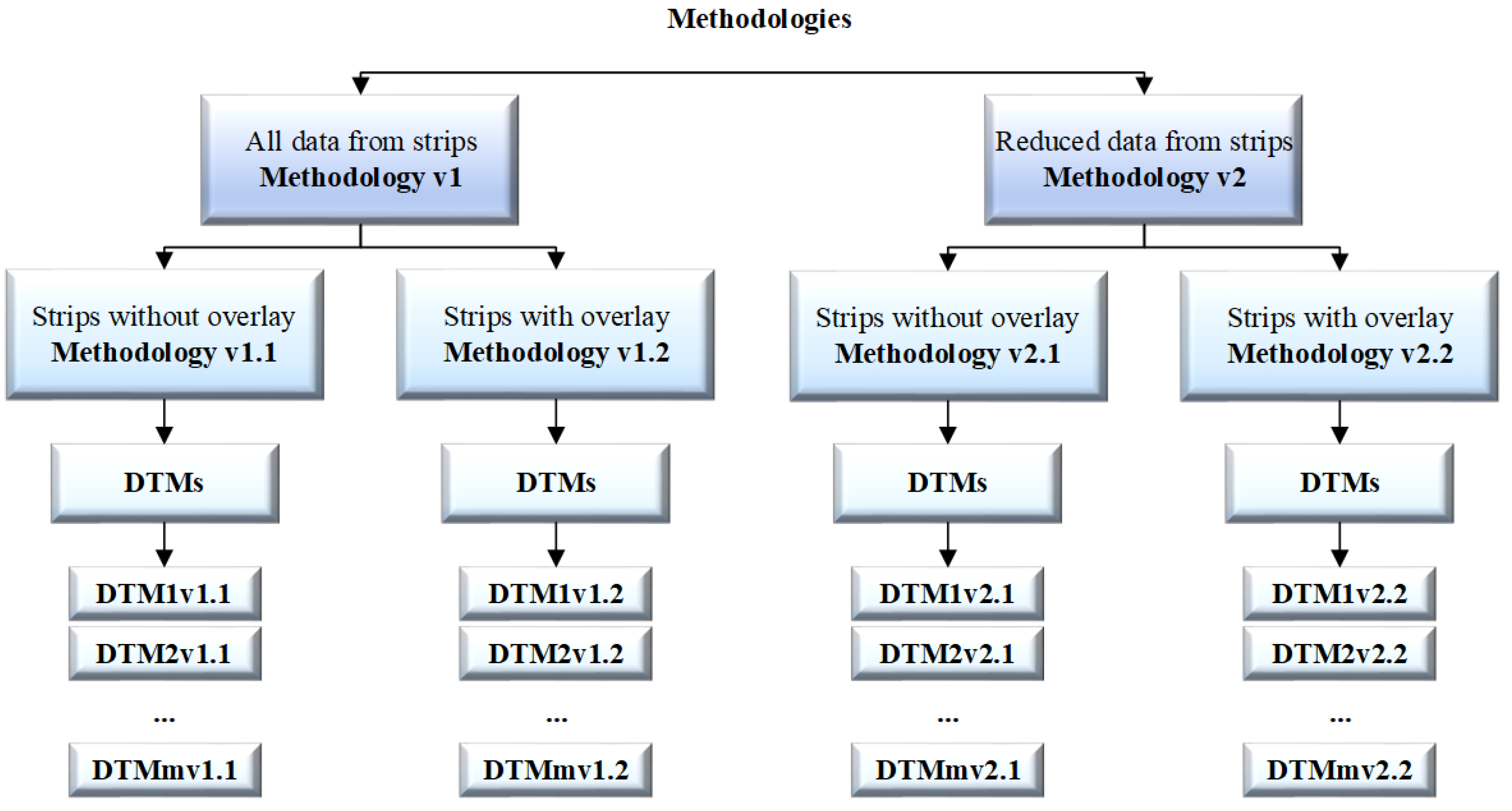
DTMmv2.1 and DTMmv2.2 were obtained for methodologies v2.1 and v2.2, and DTMv2.1 and DTMv2.2 were obtained as a sum of partial DTMs, respectively. The scheme for the proposed methodologies is presented in Figure 2.
Additionally, for comparison, DTMs were generated from all the data (100%) and from all the data after reduction (2%):
(a)
DTM100% = whole DTMv1.1 = whole DTMv1.2.
(b)
DTM2% = whole DTMv2.1 = whole DTMv2.2.
Our approach used the OptD reduction method and the kriging interpolation method.

2.3.3. OptD method

The main aim of OptD method was the reduction of the set of measurement observations. The degree of reduction was determined by setting prior, the reduction optimization criterion (c) (e.g., the number of observations in the dataset that the user required after reduction). Reduction itself was based on the cartographic generalization method. The area of interest was divided on measuring strips L. Within each L, the relative position of the points to each other was considered. The way how the points were tested in the context of being removed or preserved in the dataset depended on the tolerance range t related to the chosen cartographic generalization method. The width of L and t are iteratively changed until the optimization criterion was achieved. In result, there were different levels of reduction in the individual parts of the processing area: There were more points in the detailed part of the scanned object and much less within uncomplicated structures or areas. Only those points that were significant remained. This method has been described in detail in [35,36,37].
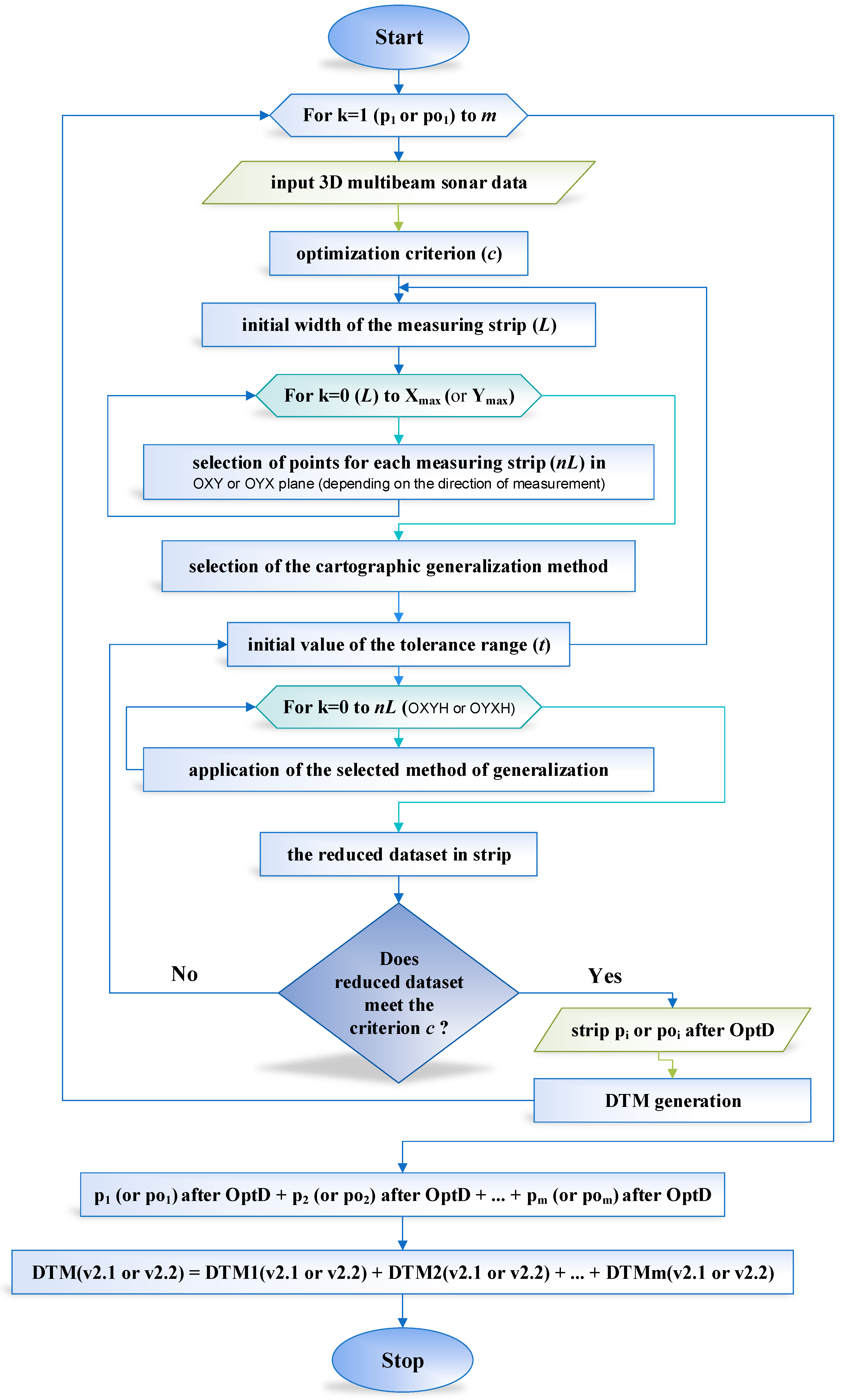
Previous applications of the OptD method consisted of processing the entire data set (airborne laser scanning—ALS, terrestrial laser scanning—TLS, mobile laser scanning—MLS). In the case of MBES, the strips with observations were reduced in almost real time and happened in stages. The OptD method was modified for this purpose. This modification relied on introducing in the OptD method a loop (FOR instruction) for fragmentary data processing. The methodology of processing MBES based on the modified OptD method is presented in Figure 3.
The strip’s width can be determined or set in relation to the measuring speed. The first measurement strip is reduced while the next strip is acquired. The second strip is attached to the previous reduced strip, and then the second is reduced while the third is obtained and so on, until the measurement is finished. Reduction conducted within each of the separated strips is based on the Douglas–Peucker cartographic generalization method [45,46]. The process can be performed for strips without overlay (methodology v2.1) or strips with overlay (methodology v2.2). Finally, we obtained a whole data set consisting of reduced strips.
(a)
For methodology v2.1, the whole dataset after reduction = p1 after OptD + p2 after OptD + … + pm after OptD
(b)
For methodology v2.2, the whole dataset after reduction = po1 after OptD + po2 after OptD + … + pom after OptD
In both versions, the optimization criterion, c, was adopted, which controls the reduction rate. For simplicity, this criterion was given as a percentage of points in the set after reduction. In this work, c = 2% was used, which is a high reduction rate. For almost real-time processing, processing time was important. Reduction decreased the number of observations, which substantially shortened the next process, DTM, and depth area generation. To generate DTM in almost real time, the kriging method was used.
In methodology v2.1, DTM1v2.1 was generated based on a reduced set with observations from the first measurement strip, p1. DTM2v2.1 was generated from p2 after the reduction, and the last interpolated node points were in the place where the DTM2v2.1 and DTM1v2.1 nodes coincided. The DTM3v2.1 nodes coincided with the nodes of the next DTM, DTM4v2.1, and the previous DTM, DTM2 v2.1, and so on. Methodology v2.2 used a similar process for strips with overlay.
Finally, the method gave the following models.
(a)
For v2.1, the whole DTMv2.1 = DTM1v2.1 + DTM2v2.1 + … + DTMmv2.1
(b)
For v2.2, the whole DTMv2.2 = DTM1v2.2 + DTM2v2.2 + … + DTMmv2.2
In addition to the DTMs generated by methodologies v2.1 and v2.2, DTMv2.1 and DTMv2.2 were obtained from the whole dataset after reduction. For comparison, using methodology v1, DTMmv1.1 and DTMmv1.2 and DTMv1.1 and DTMv1.2 were also generated.

2.3.4. Reduction

The methodology v1 test area was divided into strips with no overlay between them. The scheme for this division (methodology v1.1) is shown in Figure 4a and that for methodology v1.2, in which strips are selected with overlay, is shown in Figure 4b.
After the measurement was completed, we obtained a set of observations (Figure 5).
The statistical characteristics of the datasets obtained by methodology v1 are shown in Table 1. Each dataset represented an individual strip, pi characterized by number of points in the dataset, and the minimum and maximum height of points. Additionally, information about range and standard deviation of height was included. They allowed us to initially assess the fragments of measured areas.
In methodology v2, the original dataset was optimized using the OptD method. As in the previous case, the test area was divided into strips with and without overlay, and the variants are shown in Figure 6 and Figure 7.
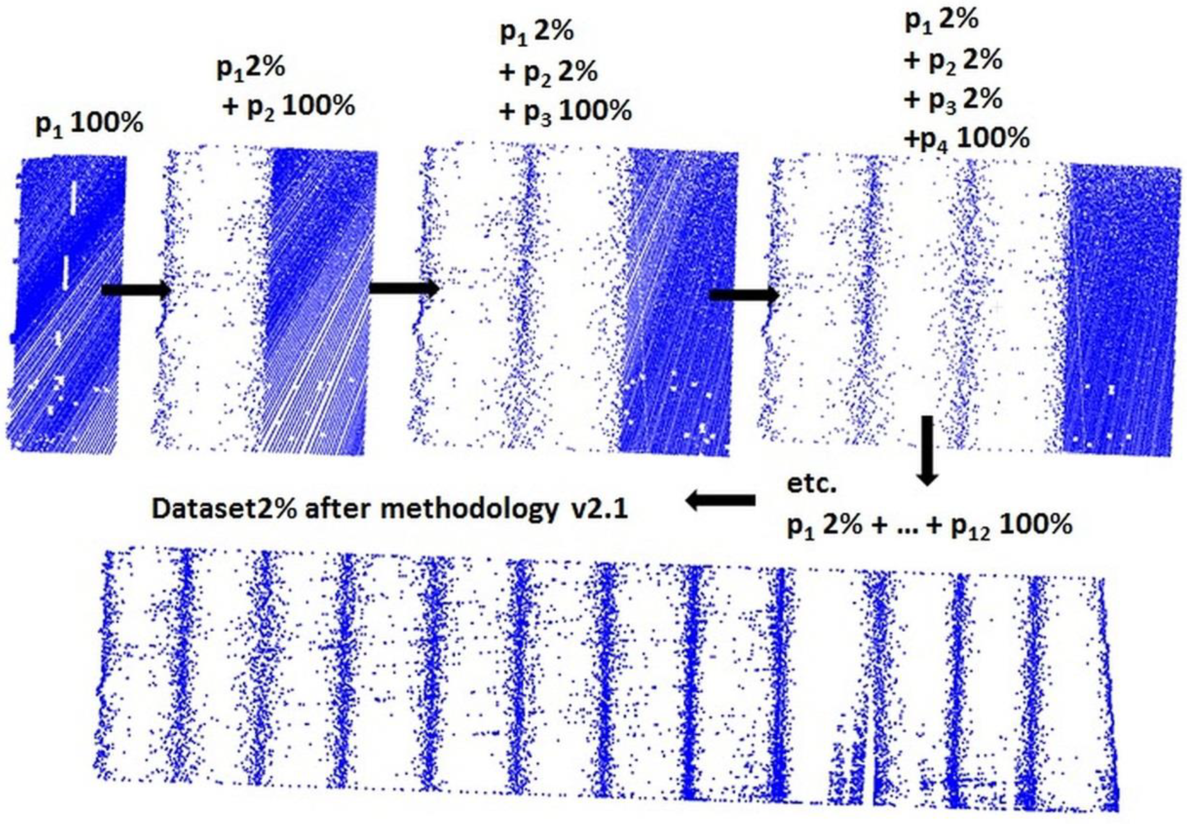
Figure 6 and Figure 7 show the difference between methodology v2.1 and v2.2. In the case of v. 2.1, there are more points where the strips contact each other than in the middle of the strips. However, in the case of v2.2 more points are in the entire overlay area.
The appearance of the whole dataset after reduction conducted using the same optimization criterion (c = 2%) is shown in Figure 8. The time required for the reduction of the whole set to 2% of the original set was about 20 s, which is acceptable for comparative navigation.
In the case of reducing the whole data set presented in Figure 8, we observed that the points remained in characteristic places of the studied area.
The statistical characteristics of the datasets obtained by methodology v2 are shown in Table 2.
The average data acquisition time in strips of 20 m at a measuring unit speed of 4 knots was about 20 s. The reduction within strips without overlay took 4–7 s, whereas for strips with overlay it took 6–9 s. The data processing time was much faster than for that of obtaining one strip.

3. Results

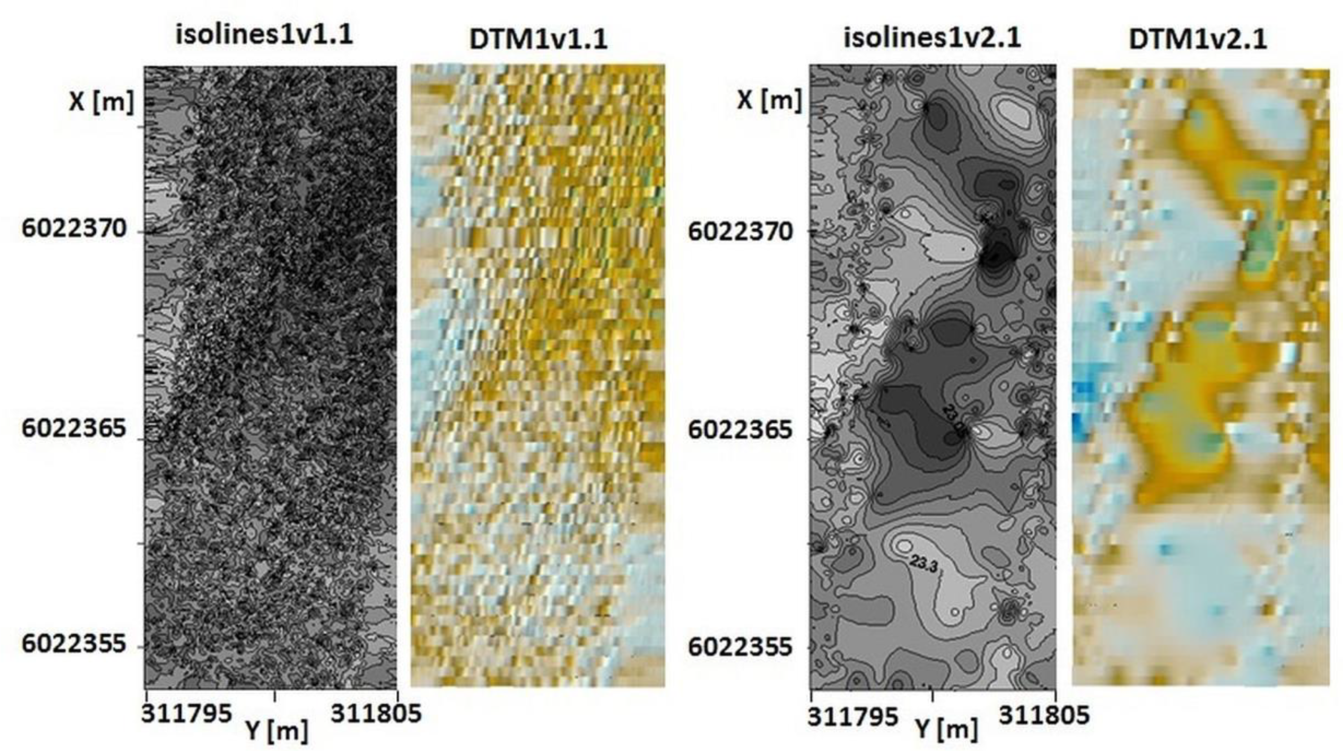
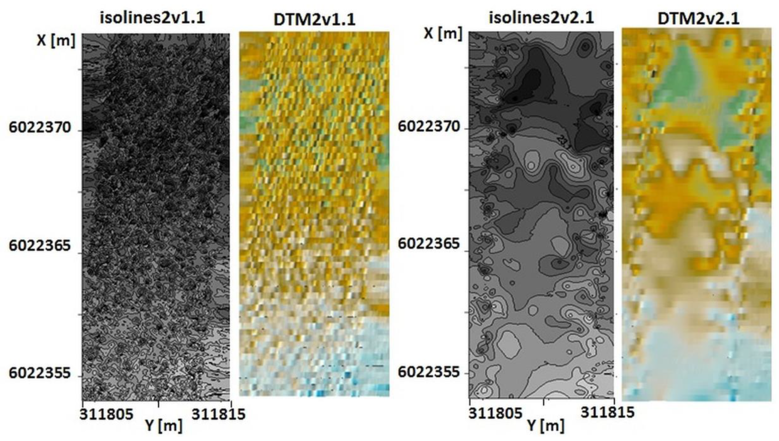
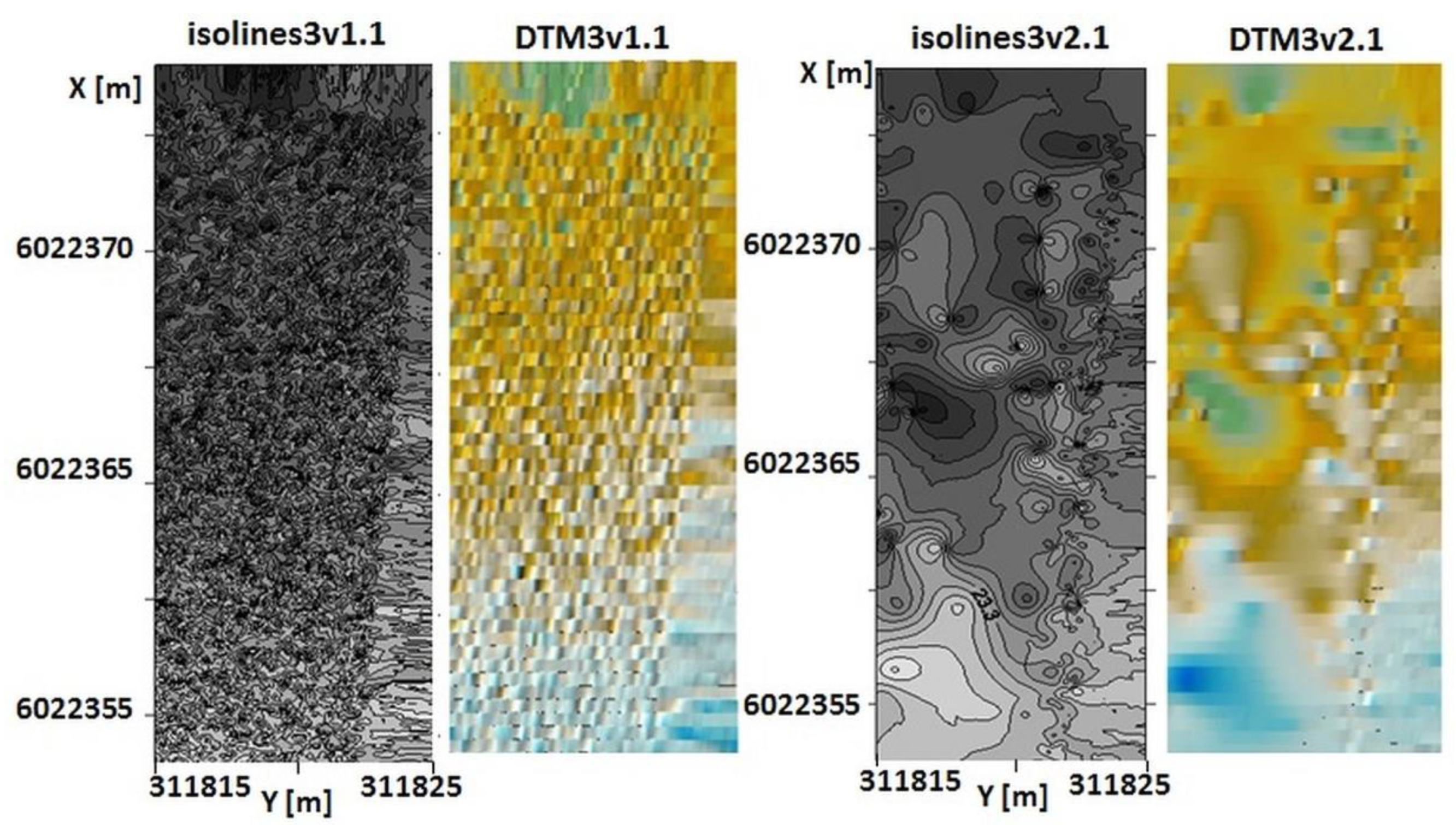
Each dataset representing strips pi and poi was used for DTM generation. The DTMs generated for strips p1, p2, and p3 are shown in Figure 9, Figure 10 and Figure 11, respectively. Next to DTMs, corresponding to them isoline maps are attached. They show, how the fragment of measured bottom of the lake look alike, when methodologies v1.1 and v2.1 were applied.
The generated DTMs and isolines maps were more readable in the case of v2.1. Fewer data has made the isoline image easier to read. Visibility of places with great depths was definitely better. Therefore, it was easier to assess the nature of the bottom from the DTMs generated by methodology v2.1. The statistical characteristics of the DTMs are presented in Table 3. As can be seen, DTMs from both methodologies v1.1 and v2.1 do not show significant statistical differences. In height, observed differences usually were about 2–3cm. For DTM4 and DTM6 they equaled −6 cm and 5 cm, respectively. This may indicated, on existence of some items on the bottom of the lake, that reduction allowed us to notice. The standard deviations calculated for DTMs generated from original dataset was usually smaller, about 1 cm in comparison to standard deviations corresponding to DTMs obtained from reduced datasets.
The total generation time for DTMv1.1 was 159 s, whereas that for DTMv2.1 was 126 s.
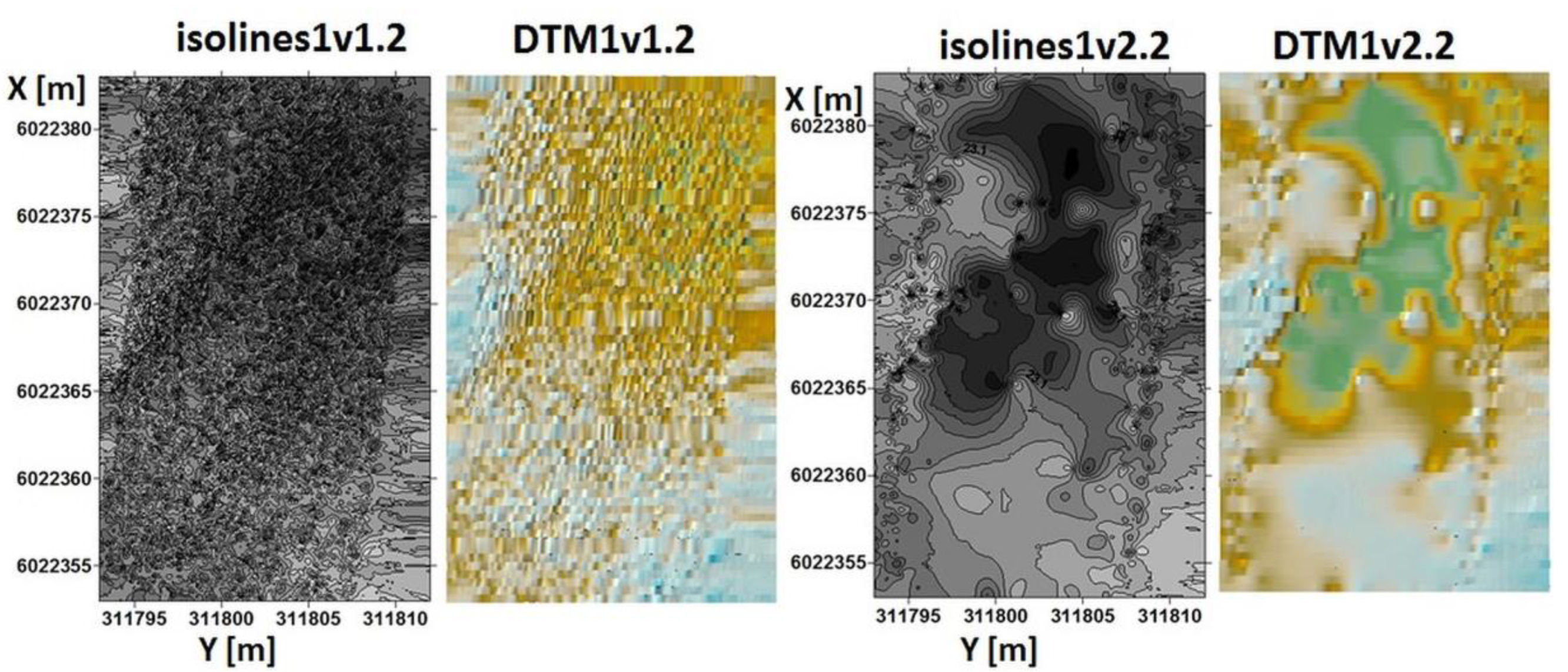
The DTMs generated for strips p1, p2, and p3 are presented Figure 11, Figure 12, Figure 13 and Figure 14.
Analyzing Figure 12, Figure 13 and Figure 14, it can be stated, as in the case of v2.1, that methodology v2.2 gave better results in terms of visibility and effectiveness of generated isolines maps and DTMs. In the figures showing the results of processing with the new v2.2 methodology, it was easier to read shallow and deep places. Methodology v1.2 figures were hard to read, and the isolines map were difficult to analyze.
The statistical characteristics of the DTMs are presented in Table 4.
The generation time for DTMv1.2 was 260 s, whereas that for DTMv2.2 was 201 s. Analyzing the statistical characteristics of DTMs obtained in methodologies v1.2 and v2.2, the trend can be observed. DTMs generated on the basis of the reduced dataset were about 1 cm higher than corresponding DTMs obtained from original measurement data.
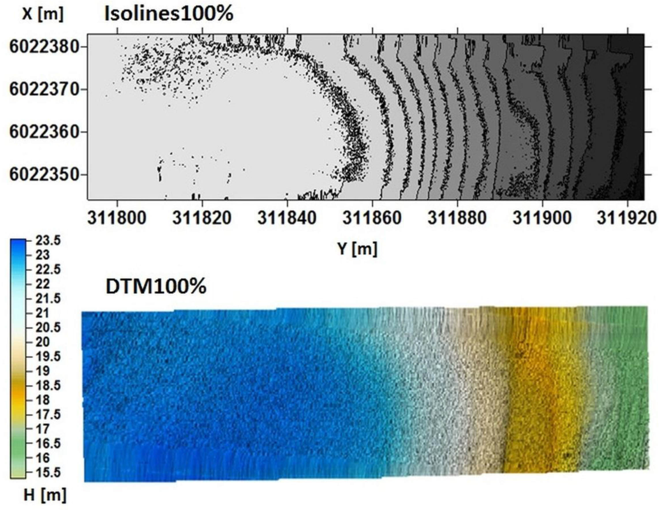
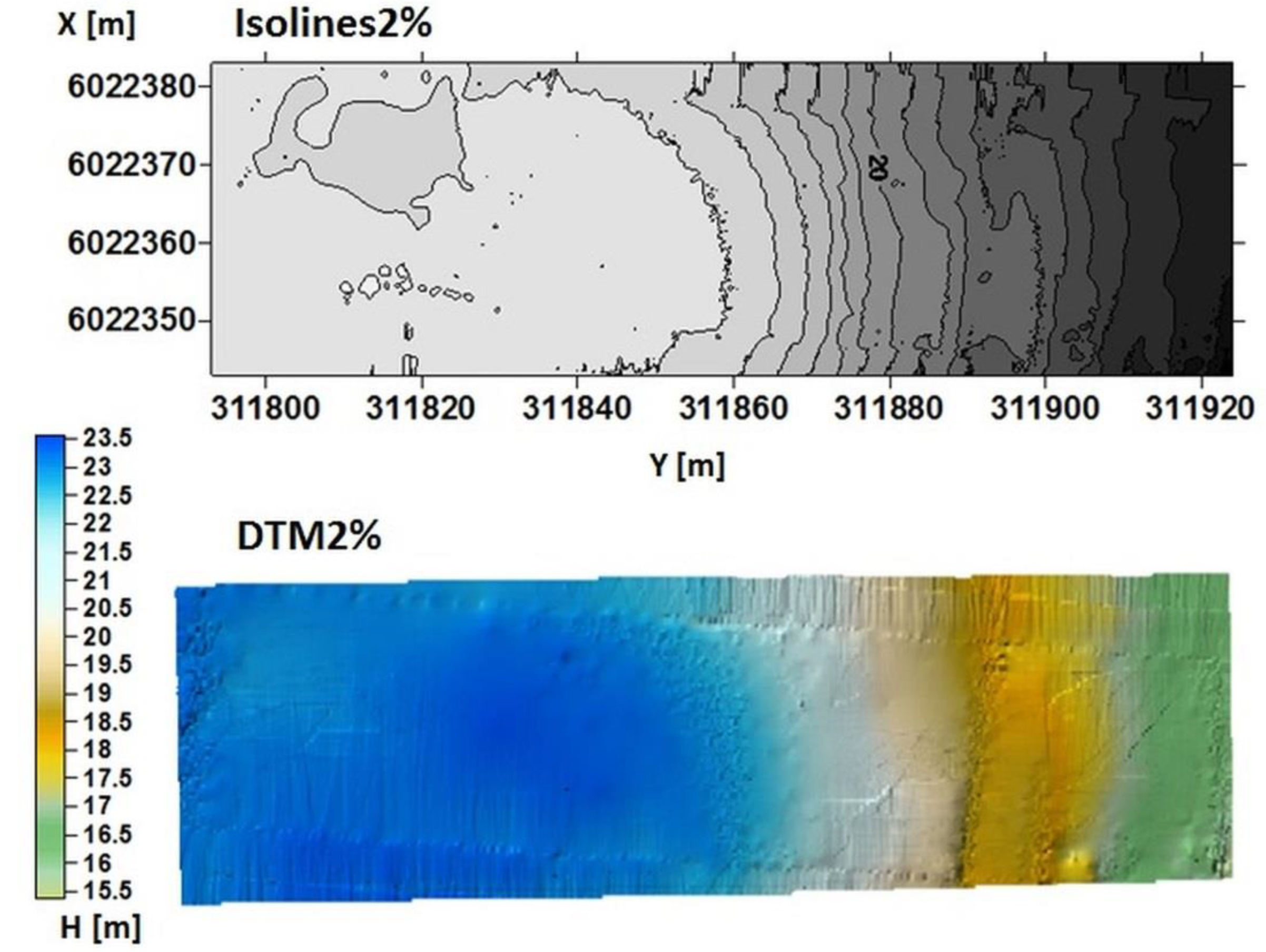
DTM 100% and DTM 2% were also generated (Figure 15 and Figure 16).
In Figure 15 and Figure 16, the conclusion about a more readable isoline map was repeated. Figure Isolines2% (Figure 16) shows areas of depth in the test area better than Isolines100% in Figure 15.
The statistical characteristics of the isolines2%, DTM2%, isolines100% and DTM100% are presented in Table 5.
The total development time of the whole set was 508 s, consisting of 240 s acquisition time of the whole set and 268 s DTM100% generation time. The total development time of the reduced set was 410 s, consisting of 240 s acquisition time of the whole set, 20 s reduction of the set to 2% of the original set, and 150 s DTM2% generation time.
To assess how the DTM strips fit together, the height differences at the corresponding nodes between adjacent strips were calculated. The results for methodologies v1 and v2 are shown in Table 6 and Table 7, respectively.
The statistical characteristics of the height differences for methodologies v1 and v2 are shown in Table 8 and Table 9, respectively.
Table 10 shows the differences between statistical characteristics for height differences between methodologies v1 and v2.
Both methodologies gave similar results; the differences between almost all the statistical characteristics were close to zero. However, the difference for ΔH min. was larger (from −0.25 to 0.14 m) because some points representing an object with various values of H may be near the area where adjacent strips are coincident. Therefore, the content of the set processed by the OptD method was different. Nonetheless, data reduction by the OptD method made the main features in the modeled areas clearer (Figure 9, Figure 10, Figure 11, Figure 12, Figure 13 and Figure 14).
The differences in statistical characteristics for height differences between using strips with and without overlay for methodology v2 are shown in Table 11. The majority of values were from −0.01 to 0.08 m, indicating that there were no significant differences between the approaches. However, the processing time for strips with overlay was longer than for strips without overlay. Therefore, the methodology based on data reduction and the variant that uses strips without overlays are suitable for depth area calculation.

4. Discussion

The new approach of methodology for processing MBES big data proposed by the authors was based on fragmentary 3D multibeam sonar data processing conducted in almost real time. All stages of standard methodology were performed not after acquisition of the whole dataset but in time, the fragments of data were acquired. While the one fragment of data was processed (execution of all stages: Reduction, DTM generation, isolines generation, analysis) the next fragment was obtained.
The most important step during the processing was reduction, because a reduced number of data allowed faster 3D bottom model generation, which can be compared with other types of data within terrain reference navigation.
Various tests can be found in the literature to speed up the calculation time of big data, e.g., parallel programming can be used with compute unified device architecture (CUDA). Using CUDA in processing of big datasets was tested, among others, by [47,48,49]. Within these works, tests on the possibility of using CUDA to generate a digital elevation model were performed. To speed up calculations there was also possibility to use artificial neural networks for modeling sea bottom shape, as these also continually implemented a surface approximation process [50,51]. These methods processed the entire dataset upon completion of the measurement. The use of these methods in almost real time was difficult, so in the new development methodology, we proposed using the OptD method.
The time needed to reduce the 3D multibeam sonar dataset based on OptD method with optimization criterion of 2% in strips was 4–7 s, whereas for strips with overlay it took 6–9 s. Such time can be considered as insignificant compared to the entire time needed for processing the whole data set. Moreover, the benefit of the reduction was a shorter time needed to generate the model. The times were as follows:
  • The total generation time for DTMv1.1 was 159 s, whereas that for DTMv2.1 was 126 s.
  • The generation time for DTMv1.2 was 260 s, whereas that for DTMv2.2 was 201 s.
  • The time needed for DTM generation was 268 s for DTM100% and 150 s for DTM2%.
Thus, the longest time was needed to generate a DTM100%. In all other cases, the time was shorter. The shortest time was needed for DTMv2.1 generation (the version with strips without overlay and with processing based on OptD method). The processing time depended on performed computer equipment and software. It is important, however, that the reduction algorithms, whose task is to speed up the development time, were uncomplicated and easy to implement.
The proposed solution also enables ongoing control during measurement. Acquired data were observed and initially analyzed in almost real time, therefore, if there was need, measurement can be repeated, completed or omitted in the selected area. Therefore, the presented approach can save time, labor, space on disks, etc.

5. Conclusions

For comparative navigation, data from MBES was processed by a new methodology which consisted of the OptD method to reduce the number of observations and generate DTMs representing measured fragments of the bottom of the area in almost real time. The data was then used to perform depth area calculations. The methodologies were based on fragmentary processing of observations organized in strips with or without overlay. Our analysis showed that using strips without overlay and with reduction by the OptD method (methodology 2.1) was an efficient, fast way to obtain data appropriate for 3D model generation that can be compared with a reference chart, such as bENCs. A major advantage of our method is that only points containing relevant information about depth differences are used for DTM construction and unimportant points belonging to flat areas are omitted. The resulting depth model of the bottom forms the first layer of a multi-layered model of the reference image bottom, which in many methods there is the only one layer. For comparative navigation based on the depth model above the flat bottom, the system cannot determine the position and additional information is required. For example, subsequent layers could be a bottom object layer and a layer containing information about the type of bottom. The layer containing characteristic points and bottom objects will use the same reduced points as the depth layer, allowing the analysis of data in semi-real time.
The general conclusions can be formulated as follows:
  • The new methodology is dedicated for 3D multibeam sonar data.
  • The new approach consists of the following steps: Acquisition the fragment of data, reducing data, and 3D model generation.
  • At the same time, the one fragment of data was processed with a new methodology, the next fragment of data was measured. This approach allows fast processing.
  • The generated DTMs or isolines maps can be simultaneously compared with existing maps (for example bENCs).
  • The time needed for fragmentary processing of 3D multibeam sonar data is shorter than the time needed for processing the whole data set.
  • The navigator has full control over the number of observations and the obtained DTMs are of good quality. In the case of isolines, mapping the obtained results shows that isolines generated by way of the OptD method are more readable and these isolines present more visible depths.

Author Contributions

Conceptualization, A.S. and A.S.-Ż.; methodology, W.B.-B.; bibliography review, A.S. and W.B.-B.; acquisition, analysis, and interpretation of data, A.S., W.M. and M.W.; writing—original draft preparation, A.S., A.S.-Ż. and W.B.-B.; writing—review and editing, A.S., W.M. and M.W.

Funding

This study was funded by the European Regional Development Fund under the 2014–2020 Operational Programme Smart Growth as part of the project “Developing of autonomous/remote operated surface platform dedicated hydrographic measurements on restricted reservoirs” implemented as part of the National Centre for Research and Development competition, INNOSBZ.

Acknowledgments

National Centre for Research and Development No. POIR.01.02.00-00-0074/16.

Conflicts of Interest

The author(s) declare(s) that they have no conflicts of interest regarding the publication of this paper.

References

  1. Chen, P.; Li, Y.; Su, Y.; Chen, X.; Jiang, Y. Review of AUV Underwater Terrain Matching Navigation. J. Navig. 2015, 68, 1155–1172. [Google Scholar] [CrossRef]
  2. Chen, P.-Y.; Li, Y.; Su, Y.-M.; Chen, X.-L.; Jiang, Y.-Q. Underwater terrain positioning method based on least squares estimation for AUV. China Ocean Eng. 2015, 29, 859–874. [Google Scholar] [CrossRef]
  3. Claus, B.; Bachmayer, R. Terrain-aided Navigation for an Underwater Glider. J. Field Robot. 2015, 32, 935–951. [Google Scholar] [CrossRef]
  4. Hagen, O.; Anonsen, K.; Saebo, T. Toward Autonomous Mapping with AUVs—Line-to-Line Terrain Navigation. In Proceedings of the Oceans 2015-MTS/IEEE Washington, Washington, DC, USA, 19–22 October 2015. [Google Scholar]
  5. Jung, J.; Li, J.; Choi, H.; Myung, H. Localization of AUVs using visual information of underwater structures and artificial landmarks. Intell. Serv. Robot. 2017, 10, 67–76. [Google Scholar] [CrossRef]
  6. Salavasidis, G.; Harris, C.; McPhail, S.; Phillips, A.B.; Rogers, E. Terrain Aided Navigation for Long Range AUV Operations at Arctic Latitudes. In Proceedings of the 2016 IEEE/OES Autonomous Underwater Vehicles (AUV), Tokyo, Japan, 6–9 November 2016; pp. 115–123. [Google Scholar]
  7. Li, Y.; Ma, T.; Wang, R.; Chen, P.; Zhang, Q. Terrain Correlation Correction Method for AUV Seabed Terrain Mapping. J. Navig. 2017, 70, 1062–1078. [Google Scholar] [CrossRef]
  8. Dong, M.; Chou, W.; Fang, B. Underwater Matching Correction Navigation Based on Geometric Features Using Sonar Point Cloud Data. Sci. Program. 2017, 2017, 7136702. [Google Scholar] [CrossRef]
  9. Song, Z.; Bian, H.; Zielinski, A. Application of acoustic image processing in underwater terrain aided navigation. Ocean Eng. 2016, 121, 279–290. [Google Scholar] [CrossRef]
  10. Ramesh, R.; Jyothi, V.B.N.; Vedachalam, N.; Ramadass, G.; Atmanand, M. Development and Performance Validation of a Navigation System for an Underwater Vehicle. J. Navig. 2016, 69, 1097–1113. [Google Scholar] [CrossRef] [Green Version]
  11. Li, Y.; Ma, T.; Chen, P.; Jiang, Y.; Wang, R.; Zhang, Q. Autonomous underwater vehicle optimal path planning method for seabed terrain matching navigation. Ocean Eng. 2017, 133, 107–115. [Google Scholar] [CrossRef]
  12. Li, Y.; Ma, T.; Wang, R.; Chen, P.; Shen, P.; Jiang, Y. Terrain Matching Positioning Method Based on Node Multi-information Fusion. J. Navig. 2017, 70, 82–100. [Google Scholar] [CrossRef]
  13. Stuntz, A.; Kelly, J.S.; Smith, R.N. Enabling Persistent Autonomy for Underwater Gliders with Ocean Model Predictions and Terrain-Based Navigation. Front. Robot. AI 2016, 3, 23. [Google Scholar] [CrossRef]
  14. Wang, L.; Yu, L.; Zhu, Y. Construction Method of the Topographical Features Model for Underwater Terrain Navigation. Pol. Marit. Res. 2015, 22, 121–125. [Google Scholar] [CrossRef] [Green Version]
  15. Wei, F.; Yuan, Z.; Zhe, R. UKF-Based Underwater Terrain Matching Algorithms Combination. In Proceedings of the 2015 International Industrial Informatics and Computer Engineering Conference, Xi’an, China, 10–11 January 2015; pp. 1027–1030. [Google Scholar]
  16. Zhou, L.; Cheng, X.; Zhu, Y. Terrain aided navigation for autonomous underwater vehicles with coarse maps. Meas. Sci. Technol. 2016, 27, 095002. [Google Scholar] [CrossRef]
  17. Zhou, L.; Cheng, X.; Zhu, Y.; Dai, C.; Fu, J. An Effective Terrain Aided Navigation for Low-Cost Autonomous Underwater Vehicles. Sensors 2017, 17, 680. [Google Scholar] [CrossRef] [PubMed]
  18. Zhou, L.; Cheng, X.; Zhu, Y.; Lu, Y. Terrain Aided Navigation for Long-Range AUVs Using a New Bathymetric Contour Matching Method. In Proceedings of the 2015 IEEE International Conference on Advanced Intelligent Mechatronics (AIM), Busan, Korea, 7–11 July 2015. [Google Scholar]
  19. Calder, B.R.; Mayer, L.A. Automatic processing of high-rate, high-density multibeam echosounder data. Geochem. Geophys. Geosyst. 2003, 4, 1048. [Google Scholar] [CrossRef]
  20. Kulawiak, M.; Lubniewski, Z. Processing of LiDAR and multibeam sonar point cloud data for 3D surface and object shape reconstruction. In Proceedings of the 2016 Baltic Geodetic Congress (BGC Geomatics), Gdańsk, Poland, 2–4 June 2016. [Google Scholar] [CrossRef]
  21. Maleika, W. Moving Average Optimization in Digital Terrain Model Generation Based on Test Multibeam Echosounder Data. Geo Mar. Lett. 2015, 35, 61–68. [Google Scholar] [CrossRef]
  22. Maleika, W. The Influence of the Grid Resolution on the Accuracy of the Digital Terrain Model Used in Seabed Modelling. Mar. Geophys. Res. 2015, 36, 35–44. [Google Scholar] [CrossRef]
  23. Wlodarczyk-Sielicka, M. Interpolating Bathymetric Big Data for an Inland Mobile Navigation System. Inf. Technol. Control. 2018, 47, 338–348. [Google Scholar] [CrossRef]
  24. Wlodarczyk-Sielicka, M.; Wawrzyniak, N. Problem of Bathymetric Big Data Interpolation for Inland Mobile Navigation System. In Communications in Computer and Information Science, Proceedings of the 23rd International Conference on Information and Software Technologies (ICIST 2017), Druskininkai, Lithuania, 12–14 October 2017; Springer: Cham, Switzerland, 2017; Volume 756, pp. 611–621. [Google Scholar] [CrossRef]
  25. Wlodarczyk-Sielicka, M.; Lubczonek, J. The Use of an Artificial Neural Network to Process Hydrographic Big Data during Surface Modeling. Computer 2019, 8, 26. [Google Scholar] [CrossRef]
  26. Rezvani, M.-H.; Sabbagh, A.; Ardalan, A.A. Robust Automatic Reduction of Multibeam Bathymetric Data Based on M-estimators. Mar. Geod. 2015, 38, 327–344. [Google Scholar] [CrossRef]
  27. Yang, F.; Li, J.; Han, L.; Liu, Z. The filtering and compressing of outer beams to multibeam bathymetric data. Mar. Geophys. Res. 2013, 34, 17–24. [Google Scholar] [CrossRef]
  28. Zhang, T.; Xu, X.; Xu, S. Method of establishing an underwater digital elevation terrain based on kriging interpolation. Measurement 2015, 63, 287–298. [Google Scholar] [CrossRef]
  29. Wlodarczyk-Sielicka, M. Importance of Neighborhood Parameters During Clustering of Bathymetric Data Using Neural Network. In Communications in Computer and Information Science, Proceedings of the 22nd International Conference on Information and Software Technologies (ICIST 2016), Druskininkai, Lithuania, 13–15 October 2016; Springer: Cham, Switzerland, 2016; Volume 639, pp. 441–452. [Google Scholar] [CrossRef]
  30. Lubczonek, J.; Borawski, M. A New Approach to Geodata Storage and Processing Based on Neural Model of the Bathymetric Surface. In Proceedings of the 2016 Baltic Geodetic Congress (BGC Geomatics), Gdansk, Poland, 2–4 June 2016; pp. 1–7. [Google Scholar] [CrossRef]
  31. Specht, C.; Świtalski, E.; Specht, M. Application of an Autonomous/Unmanned Survey Vessel (ASV/USV) in Bathymetric Measurements. Pol. Marit. Res. 2017, 24, 36–44. [Google Scholar] [CrossRef] [Green Version]
  32. Moszynski, M.; Chybicki, A.; Kulawiak, M.; Lubniewski, Z. A novel method for archiving multibeam sonar data with emphasis on efficient record size reduction and storage. Pol. Marit. Res. 2013, 20, 77–86. [Google Scholar] [CrossRef]
  33. Kogut, T.; Niemeyer, J.; Bujakiewicz, A. Neural networks for the generation of sea bed models using airborne lidar bathymetry data. Geod. Cartogr. 2016, 65, 41–54. [Google Scholar] [CrossRef] [Green Version]
  34. Aykut, N.O.; Akpınar, B.; Aydın, Ö. Hydrographic data modeling methods for determining precise seafloor topography. Comput. Geosci. 2013, 17, 661–669. [Google Scholar] [CrossRef]
  35. Blaszczak-Bak, W. New Optimum Dataset method in LiDAR processing. Acta Geodyn. Geomater. 2016, 13, 379–386. [Google Scholar] [CrossRef]
  36. Błaszczak-Bąk, W.; Koppanyi, Z.; Toth, C. Reduction Method for Mobile Laser Scanning Data. ISPRS Int. J. Geo Inf. 2018, 7, 285. [Google Scholar] [CrossRef]
  37. Błaszczak-Bąk, W.; Sobieraj-Żłobińska, A.; Kowalik, M. The OptD-multi method in LiDAR processing. Meas. Sci. Technol. 2017, 28, 75009. [Google Scholar] [CrossRef]
  38. Kazimierski, W.; Wlodarczyk-Sielicka, M. Technology of Spatial Data Geometrical Simplification in Maritime Mobile Information System for Coastal Waters. Pol. Marit. Res. 2016, 23, 3–12. [Google Scholar] [CrossRef] [Green Version]
  39. Stateczny, A.; Gronska-Sledz, D.; Motyl, W. Precise Bathymetry as a Step Towards Producing Bathymetric Electronic Navigational Charts for Comparative (Terrain Reference) Navigation. J. Navig. 2019. [Google Scholar] [CrossRef]
  40. Borkowski, P.; Pietrzykowski, Z.; Magaj, J.; Mąka, M. Fusion of data from GPS receivers based on a multi-sensor Kalman filter. Transp. Probl. 2008, 3, 5–11. [Google Scholar]
  41. Donovan, G.T. Position Error Correction for an Autonomous Underwater Vehicle Inertial Navigation System (INS) Using a Particle Filter. IEEE J. Ocean. Eng. 2012, 37, 431–445. [Google Scholar] [CrossRef]
  42. Wawrzyniak, N.; Stateczny, A. MSIS Image Positioning in Port Areas with the Aid of Comparative Navigation Methods. Pol. Marit. Res. 2017, 24, 32–41. [Google Scholar] [CrossRef]
  43. Ping DSP, Products Description. Available online: http://www.pingdsp.com/3DSS-DX-450 (accessed on 9 May 2019).
  44. Stateczny, A.; Wlodarczyk-Sielicka, M.; Gronska, D.; Motyl, W. Multibeam Echosounder and Lidar in Process of 360° Numerical Map Production for Restricted Waters with Hydrodron. In Proceedings of the 2018 Baltic Geodetic Congress (BGC Geomatics) Gdansk, Olsztyn, Poland, 21–23 June 2018. [Google Scholar] [CrossRef]
  45. Douglas, D.; Peucker, T. Algorithms for the reduction of the number of points required to represent a digitized line or its caricature. Cartographica 1973, 10, 112–122. [Google Scholar] [CrossRef]
  46. Fei, L.; Jin, H. A three-dimensional Douglas–Peucker algorithm and its application to automated generalization of DEMs. Int. J. Geogr. Inf. Sci. 2009, 23, 703–718. [Google Scholar] [CrossRef]
  47. Zeng, X.; He, W. GPGPU Based Parallel processing of Massive LiDAR Point Cloud. In Proceedings of the MIPPR 2009: Medical Imaging, Parallel Processing of Images, and Optimization Techniques. International Society for Optics and Photonics, Yichang, China, 30 October–1 November 2009; Volume 7497. [Google Scholar]
  48. Chen, Y. High Performance Computing for Massive LiDAR Data Processing with Optimized GPU Parallel Programming. Master’s Thesis, The University of Texas at Dallas, Richardson, TX, USA, 2012. [Google Scholar]
  49. Cao, J.; Cui, H.; Shi, H.; Jiao, L. Big Data: A Parallel Particle Swarm Optimization-Back-Propagation Neural Network Algorithm Based on MapReduce. PLoS ONE 2016, 11, e0157551. [Google Scholar] [CrossRef] [PubMed]
  50. Liu, S.; Wang, L.; Liu, H.; Su, H.; Li, X.; Zheng, W. Deriving Bathymetry from Optical Images with a Localized Neural Network Algorithm. IEEE Trans. Geosci. Remote Sens. 2018, 56, 5334–5342. [Google Scholar] [CrossRef]
  51. Lubczonek, J. Hybrid neural model of the sea bottom surface. In Lecture Notes in Computer Science, Proceedings of the International Conference on Artificial Intelligence and Soft Computing (ICAISC), Zakopane, Poland, 7–11 June 2004; Springer: Berlin/Heidelberg, Germany, 2004; Volume 3070, pp. 1154–1160. [Google Scholar]
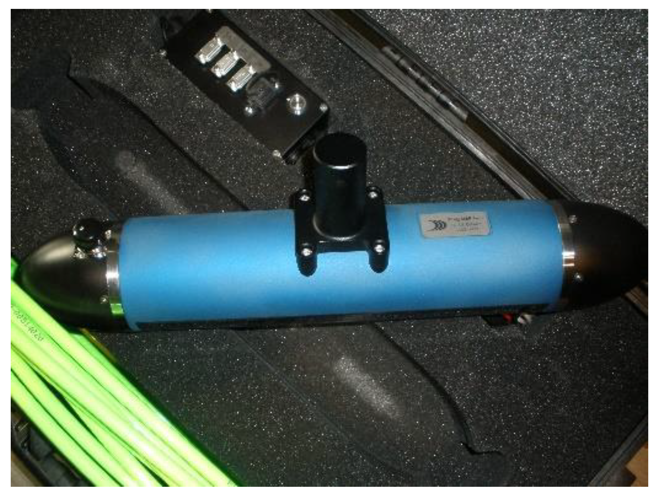
Figure 1. Photograph of the 3D Sidescan 3DSS-DX-450 sonar system (photograph: A. Stateczny).
Remotesensing 11 02245 g001
Figure 2. Scheme of the methodologies.
Remotesensing 11 02245 g002
Figure 3. Processing of multibeam echosounders (MBES) data based on the Optimum Dataset OptD method.
Remotesensing 11 02245 g003
Figure 4. Scheme of test area division into strips (a) with and (b) without overlay.
Remotesensing 11 02245 g004
Figure 5. Whole test area (694,185 points).
Remotesensing 11 02245 g005
Figure 6. Scheme of the test area division into strips without overlay (methodology v2.1).
Remotesensing 11 02245 g006
Figure 7. Scheme of test area division into strips with overlay (methodology v2.2).
Remotesensing 11 02245 g007
Figure 8. Optimized test area (13,976 points).
Remotesensing 11 02245 g008
Figure 9. Isolines1v1.1 and digital terrain model (DTM)1v1.1, and isolines1v2.1 and DTM1v2.1 generated for strip 1 (p1) by methodologies v1.1 and v2.1, respectively.
Remotesensing 11 02245 g009
Figure 10. Isolines2v1.1 and DTM2v1.1, and isolines2v2.1 and DTM2v2.1 generated for strip 2 (p2) by methodologies v1.1 and v2.1, respectively.
Remotesensing 11 02245 g010
Figure 11. Isolines3v1.1 and DTM3v1.1, and isolines3v2.1 and DTM3v2.1 generated for strip 3 (p3) by methodologies v1.1 and v2.1, respectively.
Remotesensing 11 02245 g011
Figure 12. Isolines1v1.2 and DTM1v1.2, and isolines1v2.2 and DTM1v2.2 generated for strip 1 (po1) by methodologies v1.2 and v2.2, respectively.
Remotesensing 11 02245 g012
Figure 13. Isolines2v1.2 and DTM2v1.2, and isolines2v2.2 and DTM2v2.2 generated for strip 2 (po2) by methodologies v1.2 and v2.2, respectively.
Remotesensing 11 02245 g013
Figure 14. Isolines3v1.2 and DTM3v1.2, and isolines3v2.2 and DTM3v2.2 generated for strip 3 (po3) by methodologies v1.2 and v2.2, respectively.
Remotesensing 11 02245 g014
Figure 15. Isolines100% and DTM100%.
Remotesensing 11 02245 g015
Figure 16. Isolines2% and DTM2%.
Remotesensing 11 02245 g016
Table 1. Statistical characteristics for datasets in methodology v1. (Where: H—height, R—range, STD—standard deviation).
Number of PointsH min. [m]H max. [m]R [m]STD [m]
Whole dataset69418515.0823.658.572.44
Strips without overlayp15417622.8623.540.680.08
p23510622.8623.600.740.11
p34433322.8223.580.760.12
p45357922.7523.650.900.10
p55296722.6423.520.880.11
p65549722.0423.391.350.20
p77070420.8423.142.300.40
p88496219.4822.162.680.55
p97989017.8620.422.560.49
p105321617.3518.781.430.27
p115537316.3618.041.680.33
p125438215.0817.031.950.31
Strips with overlaypo17271822.8623.540.680.09
po25607522.8223.600.780.12
po37247822.7523.650.900.11
po48093622.7323.650.920.10
po58064222.4023.521.120.14
po69002221.5023.391.890.29
po711558420.1823.162.980.62
po812289418.7522.213.460.75
po910181017.7120.422.710.56
po108481016.9218.781.860.41
po118455115.8218.042.220.44
po125459215.0817.041.960.31
Table 2. Statistical characteristics for datasets in methodology v2. (Where: H—height, R—range, STD—standard deviation).
Number of PointsH min. [m]H max. [m]R [m]STD [m]
Optimized dataset1397615.1023.578.472.86
Strips without overlayp1109122.8623.530.670.11
p270222.8623.570.710.13
p388822.8523.570.720.13
p4107122.7523.650.900.13
p5105522.7223.520.800.14
p6111122.0523.351.300.25
p7140320.8423.102.260.55
p8171019.5022.162.660.78
p9160517.8620.382.520.71
p10106617.4018.761.360.36
p11111616.3618.001.640.50
p12107915.1017.011.910.46
Strips with overlaypo1144622.8623.540.680.13
po2113222.8623.600.740.13
po3144422.8123.650.840.14
po4163322.7723.650.880.14
po5161922.4223.521.100.21
po6179421.5623.381.820.42
po7232120.2623.112.850.86
po8245618.7622.193.431.08
po9201817.7120.422.710.80
po10169116.9218.771.850.62
po11168915.9118.012.100.65
po12109415.1016.961.860.46
Table 3. Statistical characteristics for DTMmv1.1 and DTMmv2.1. (Where: H—height, STD—standard deviation).
DTMH min. [m]H max. [m]STD [m]Time [s] for Generated DTMs
DTM1v1.1
DTM1v2.1
22.88
22.85
23.48
23.47
0.08
0.09
14
14
DTM2v1.1
DTM2v2.1
22.87
22.87
23.57
23.53
0.12
0.12
12
10
DTM3v1.1
DTM3v2.1
22.83
22.83
23.54
23.54
0.13
0.14
11
9
DTM4v1.1
DTM4v2.1
22.80
22.79
23.54
23.60
0.13
0.12
15
12
DTM5v1.1
DTM5v2.1
22.67
22.65
23.51
23.51
0.12
0.13
13
11
DTM6v1.1
DTM6v2.1
22.70
22.67
23.38
23.33
0.22
0.24
14
10
DTM7v1.1
DTM7v2.1
20.79
20.77
23.12
23.12
0.44
0.47
13
9
DTM8v1.1
DTM8v2.1
19.43
19.45
22.09
22.09
0.58
0.59
14
10
DTM9v1.1
DTM9v2.1
17.99
17.96
20.40
20.37
0.55
0.55
16
12
DTM10v1.1
DTM10v2.1
17.35
17.37
18.76
18.74
0.31
0.32
12
10
DTM11v1.1
DTM11v2.1
16.37
16.36
18.02
17.99
0.39
0.40
12
9
DTM12v1.1
DTM12v2.1
15.16
15.15
17.01
17.01
0.29
0.29
13
10
Table 4. Statistical characteristics for DTMmv1.2 and DTMmv2.2. (Where: H—height, STD—standard deviation).
DTMH min. [m]H max. [m]STD [m]Time [s] for Generated DTMS
DTM1v1.2
DTM1v2.2
22.87
22.86
23.47
23.50
0.09
0.12
20
19
DTM2v1.2
DTM2v2.2
22.86
22.87
23.52
23.53
0.12
0.13
21
18
DTM3v1.2
DTM3v2.2
22.80
22.82
23.54
23.55
0.12
0.12
23
19
DTM4v1.2
DTM4v2.2
22.82
22.79
23.54
23.55
0.11
0.13
22
18
DTM5v1.2
DTM5v2.2
22.43
22.46
23.50
23.51
0.15
0.16
21
17
DTM6v1.2
DTM6v2.2
21.52
21.53
23.41
23.39
0.31
0.32
21
16
DTM7v1.2
DTM7v2.2
20.23
20.25
23.12
23.09
0.67
0.68
22
16
DTM8v1.2
DTM8v2.2
18.76
18.76
22.15
22.16
0.81
0.82
22
15
DTM9v1.2
DTM9v2.2
17.75
17.71
20.39
20.42
0.63
0.65
24
16
DTM10v1.2
DTM10v2.2
16.95
16.96
18.76
18.75
0.43
0.45
19
14
DTM11v1.2
DTM11v2.2
15.81
15.83
18.02
18.00
0.49
0.50
23
16
DTM12v1.2
DTM12v2.2
15.16
15.17
17.02
16.99
0.29
0.28
22
16
Table 5. Statistical characteristics for DTM100% and DTM2%. (Where: H—height, STD—standard deviation).
DTMH min. [m]H max. [m]STD [m]Time [s] for Generated DTMS
DTM100%
DTM2%
15.29
15.32
23.56
23.56
2.50
2.54
268
150
Table 6. Height differences between strips in methodology v1. (Where: H—height, STD—standard deviation).
ΔH min. [m]ΔH max. [m]ΔHmean [m]STD [m]
Strips without overlayp1–p2−0.320.320.010.08
p2–p3−0.220.270.000.02
p3–p4−0.370.30−0.010.08
p4–p5−0.490.28−0.020.08
p5–p6−0.360.30−0.020.07
p6–p7−0.400.32−0.030.08
p7–p8−0.600.29−0.090.13
p8–p9−0.580.27−0.060.11
p9–p10−0.800.23−0.060.11
p10–p11−0.520.19−0.080.09
p11–p12−0.430.22−0.030.07
Strips with overlaypo1–po2−0.260.220.000.05
po2–po3−0.330.330.000.05
po3–po4−0.310.25−0.010.04
po4–po5−0.260.240.000.04
po5–po6−0.280.240.000.04
po6–po7−0.370.28−0.030.07
po7–po8−0.560.21−0.040.10
po8–po9−0.430.20−0.030.07
po9–po10−0.520.24−0.030.07
po10–po11−0.380.25−0.020.05
po11–po12−0.430.42−0.010.06
Table 7. Height differences between strips in methodology v2. (Where: H—height, STD—standard deviation).
ΔH min. [m]ΔH max. [m]ΔHmean [m]STD [m]
Strips without overlayp1–p2−0.210.340.030.07
p2–p3−0.290.280.000.11
p3–p4−0.220.250.000.07
p4–p5−0.340.21−0.020.07
p5–p6−0.310.23−0.020.09
p6–p7−0.240.24−0.030.07
p7–p8−0.440.26−0.080.11
p8–p9−0.550.28−0.100.13
p9–p10−0.490.27−0.040.08
p10–p11−0.400.18−0.060.08
p11–p12−0.440.17−0.040.07
Strips with overlaypo1–po2−0.210.27−0.010.08
po2–po3−0.200.05−0.060.07
po3–po4−0.260.260.070.07
po4–po5−0.290.20−0.020.08
po5–po6−0.200.200.030.06
po6–po7−0.310.33−0.030.12
po7–po8−0.520.24−0.110.14
po8–po9−0.700.28−0.060.19
po9–po10−0.350.260.020.08
po10–po11−0.390.470.030.16
po11–po12−0.370.530.050.15
Table 8. Statistical characteristics for height differences between strips (methodology v1). (Where: H—height, STD—standard deviation).
Methodology v1
ΔH min. [m]ΔH max. [m]ΔHmean [m]STD [m]
Strips without overlayMin.−0.800.19−0.090.02
Max.−0.220.320.010.13
Mean−0.460.29−0.030.08
Standard deviation0.160.040.030.03
Strips with overlayMin.−0.560.20−0.040.04
Max.−0.260.420.000.10
Mean−0.380.26−0.010.06
Standard deviation0.100.060.010.02
Table 9. Statistical characteristics for height differences between strips (methodology v2). (H—height, STD—standard deviation).
Methodology v2
ΔH min. [m]ΔH max. [m]ΔHmean [m]STD [m]
Strips without overlayMin.−0.550.17−0.100.07
Max.−0.210.340.030.13
Mean−0.340.26−0.030.09
Standard deviation0.120.050.040.02
Strips with overlayMin.−0.700.05−0.110.06
Max.−0.200.530.070.19
Mean−0.350.28−0.010.11
Standard deviation0.150.130.050.04
Table 10. Differences between statistical characteristics for height differences between methodologies. (Where: H—height, STD—standard deviation).
Methodology v1—Methodology v2
ΔH min. [m]ΔH max. [m]ΔHmean [m]STD [m]
Strips without overlayMin.−0.250.020.01−0.05
Max.−0.01−0.02−0.020.01
Mean−0.120.020.000.00
Standard deviation0.04−0.010.000.01
Strips with overlayMin.0.140.150.07−0.03
Max.−0.05−0.11−0.07−0.09
Mean−0.03−0.02−0.01−0.05
Standard deviation−0.05−0.07−0.04−0.03
Table 11. Differences in statistical characteristics for height differences between strips with and without overlay. (Methodology v2). (where: H—height, STD—standard deviation).
Strips with Overlay—Strips without Overlay
ΔH min. [m]ΔH max. [m]ΔHmean [m]STD [m]
Min.−0.15−0.12−0.010.00
Max.0.010.190.050.06
Mean0.000.020.020.02
Standard deviation0.040.080.020.02