Abstract
Data describing aircraft position and attitude are essential to computing return positions from ranging data collected during airborne laser scanning (ALS) campaigns. However, these data are often excluded from the products delivered to the client and their recovery after the contract is complete can require negotiations with the data provider, may involve additional costs, or even be infeasible. This paper presents a rigorous, fully automated, novel method for recovering aircraft positions using only the point cloud. The study used ALS data from five acquisitions in the US Pacific Northwest region states of Oregon and Washington and validated derived aircraft positions using the smoothed best estimate of trajectory (SBET) provided for the acquisitions. The computational requirements of the method are reduced and precision is improved by relying on subsets of multiple-return pulses, common in forested areas, with widely separated first and last returns positioned at opposite sides of the aircraft to calculate their intersection, or closest point of approach. To provide a continuous trajectory, a cubic spline is fit to the intersection points. While it varies by acquisition and parameter settings, the error in the computed aircraft position seldom exceeded a few meters. This level of error is acceptable for most applications. To facilitate use and encourage modifications to the algorithm, the authors provide a code that can be applied to data from most ALS acquisitions.
1. Introduction
Airborne laser scanning (ALS), or light detection and ranging (LiDAR) as this technology is alternatively known, has been used, and often relied upon [1], to generate detailed and precise digital descriptions of ground surfaces [2], model hydrologic systems [3], assess forest above-ground biomass [4], map snow depth [5], monitor powerlines [6], and measure terrain displacement induced by seismic events [7]. Over urban landscapes, ALS has been used to delineate road networks [8], detect impervious surfaces [9], identify and describe individual trees [10,11], biomass [12], estimate leaf area index [13], identify and assess trees damaged by extreme weather [14], assess the photovoltaic potential of residential buildings [15,16], and in many other applications.
Many ALS data analyses and applications, including some of those mentioned above, require or benefit from information describing the range and pulse angle associated with each return or echo. Range, the 3D distance from the sensor to each return, is typically used to normalize recorded return intensity, a parameter associated with the backscattering attributes and ultimately characteristics of targets illuminated by laser pulses [17,18,19]. For a given beam divergence setting of the laser instrument, the calculated range to a return also provides the precise footprint of the pulse incident upon a target. The term pulse angle, defined here as the three-dimensional, angular deviation from a pulse directed perpendicularly to a horizontal plane [13], is calculated by fitting a 3D line connecting the first and last returns of the pulse. The first and last return are identified as a pair across all returns by their shared GPS time [20]. As pulses are diverted by an oscillating or rotating mirror, or other hardware component, across the trajectory of the laser instrument and airborne platform, the pulse angle changes rapidly and continuously during an acquisition. Over forested landscapes, the pulse angle is known to affect the computation of tree height, leaf area index, gap fraction, and canopy cover [21,22,23,24], all important parameters for forest resource assessment and planning. This is primarily because as the angle increases, the length of the pulse trajectory intersected by a tree crown also increases, and with it, the probability for a crown return. Conversely, the probability of a ground return decreases. This phenomenon, manifested as a horizontal displacement of ground returns with respect to returns from the canopy, is sometimes referred to as ‘LiDAR shadow’ and it is more pronounced with trees featuring a high leaf area index [13].
Unlike pulse angle, scan angle is defined as the angular deviation from a pulse directed perpendicularly to the plane of the laser instrument and its magnitude is independent of platform attitude. The scan angle pertaining to a return is a required field in all American Society for Photogrammetry and Remote Sensing (ASPRS)-compliant ALS data files (LAS) [25,26] and is recorded as a char (1-byte element) with, by convention, positive values for pulses oriented towards the port and negative values towards the starboard side of the aircraft. The latest LAS 1.4 format contains a provision for an extension of the scan angle field to 2 bytes to provide finer angle resolution. On a perfectly level flight, pulse and scan angles are theoretically identical. Discrepancies are introduced as the aircraft attitude changes during data collection.
In a typical ALS flight, the directional vectors of the airborne platform and, hence, those of the laser instrument, are recorded by an inertial measurement unit (IMU). A high-end Global Positioning System (GPS) device records positions which are improved during a post-processing phase using data from a nearby, strategically placed, ground GPS station operating during the flights. This information and the pulse directional vectors relative to and recorded by the laser instrument are combined to calculate the trajectory of each emitted pulse. The time that elapses between pulse emission and interception of backscatter pulse photons determines the range and the 3D coordinates of each return associated with a pulse. A detailed description of the process is available in [27].
The data collected during ALS operations and available as a potential deliverable includes the GPS location and IMU attitude information. These data, collectively called the aircraft trajectory, are recorded at high frequencies (~200 Hz) and are essential for the production of a point cloud from the range data recorded by the laser scanner. At this recording rate, each position represents a change of only about 30 cm along the aircraft trajectory assuming a speed of 220 km/h (119 knots). Position information in the trajectory is typically referenced in GPS week time (number of seconds from the beginning of the week, resetting, or rolling over, at 12:00 AM each Sunday). This presents challenges for acquisitions lasting more than one week because identical time stamps could refer to more than one platform position. To overcome this challenge, GPS time is typically replaced with the Adjusted GPS Time (number of seconds that have passed since the beginning of GPS time: midnight between 5 January and 6 January 1980, minus one billion seconds).
While critical for ALS data generation, platform trajectory data are not always included in data deliverables, primarily due to the absence of relevant clauses in acquisition specifications. This is the case, for example, with acquisitions supporting the United State Geological Survey (USGS) 3D Elevation Program (3DEP) [28], a substantial initiative aiming at generating high-resolution digital terrain models (DTMs) across the continental United States. A survey of data from nearly 100 ALS acquisitions stored in a portal hosted by Oregon State University (ftp://lidar.engr.oregonstate.edu, last accessed on 31 July 2019) showed that only about one in three contained platform trajectory data. Even lower, often much lower, percentages are reported in personal communications with analysts elsewhere in the United States, Canada, and Europe.
Even when trajectory data are included in deliverables, they are not necessarily in the projection of the raw return data. Many vendors have an established data processing workflow based on a projection of choice that is applied across their entire area of operations. All intermediate data products are organized in the preferred projection and are converted to the projection desired by the client just prior to delivery. Reprojection of the trajectory data to match the rest of the deliverables is often neglected. In the absence of adequate documentation regarding the registration of intermediate products, projection discrepancies can be challenging to resolve, especially when they involve datum shifts and other somewhat esoteric parameters. In addition, retrieval of trajectory data after, often long after, delivery can be logistically complicated, time consuming, and costly. Vendors may charge fees for copies of archived data, the archive could be missing, or the vendor could have ceased operations.
The goal of this study is to develop and present a new method that computes the trajectory of the laser instrument using the point cloud. We evaluate the resulting trajectories using ALS data from five acquisitions across different biomes in the United States Pacific Northwest region and compare the computed trajectory to the trajectory recorded during the data acquisition.
2. Materials and Methods
2.1. Study Area and Airborne Laser-Scanning (ALS) Data
We used ALS data from five acquisitions in the US Pacific Northwest region states of Oregon and Washington (Figure 1), titled Colville, Deschutes, McKenzie, Tillamook, and West Metro. Each represents a distinct biome. All selected data sets contained airborne platform trajectory information provided by the vendor. GPS time was recorded in the weekly format except for McKenzie, where the adjusted format was used. McKenzie was acquired with a dual laser instrument configuration and had a platform trajectory file in a projection different from the one used for the raw laser data. The Tillamook area is representative of the temperate rainforests and topography of the coastal Oregon mountain range. It is subject to intense forest management. West Metro contains portions of the cities of Portland, Beaverton, and Hillsboro, with moderate tree cover over hills and low housing density in the northeastern section, gradually leveling off to plains with sporadic trees and high housing density towards the west. The McKenzie area contains the eastern portions of the City of Springfield to the west, followed by agricultural land, and then high tree canopy cover forests to the east towards the Cascade mountain passes. The Deschutes area, part of a much larger acquisition, is located at the eastern foothills of the Cascade mountains on rolling terrain and is characterized by open stands with medium to low tree canopy cover. The Colville area is in the northeastern part of the State of Washington. It is within the Northern Rockies ecoregion and is dominated by dry highland forests [29]. Descriptive statistics of each study area are shown in Table 1. Elevation and slope metrics were calculated using 1 m digital terrain models (DTMs) generated from the ALS data. Tree canopy cover calculations used a 2 m above-ground return height cutoff value as an indicator of tree returns and, for McKenzie and West Metro, a prior elimination of returns classified as ‘building’ by a GlobalMapper 20 LiDAR module [30]. Acquisition specifications are shown in Table 2. Across all areas, pulse density, and therefore return density, is high, exceeding 7 pulses per square meter. The field-of-view, or bilateral scan angle, is lower and sidelap is higher than what is common in ALS acquisitions elsewhere. The specifications for acquisitions selected for this study are similar to those used by the Forest Service, the Oregon Department of Geology and Mineral Industries (DOGAMI), and other partners collaborating on ALS acquisition in the region. They are considered optimal for minimization of artifacts such as the laser shadows mentioned earlier.
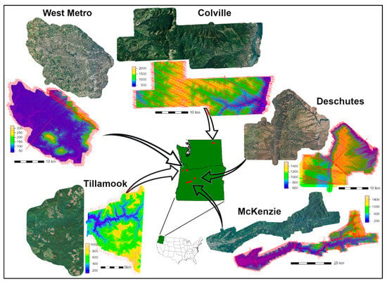
Figure 1.
Spatial distribution of study areas, each featuring National Agriculture Imagery Program (NAIP) panchromatic imagery co-temporal to the ALS data acquisition and a digital terrain model generated from the laser data with superimposed platform trajectory lines displayed in red. Scale varies across the five study areas.

Table 1.
Physiographic metrics of study areas.

Table 2.
Timing and instrument specifications of ALS acquisitions.
2.2. Pulse Returns to Ray Convergence
A laser pulse incident upon an opaque object yields a single return. When incident upon a non-solid object, such as a tree crown, each pulse will typically generate more than one return. Multiple returns can be generated from solid objects as well, if the pulse direction is nearly parallel to the object’s surface. An example for the latter case would be a pulse skimming the side of a building with one return located near the top, and one or more returns at different heights on the building’s side. As stated earlier, return coordinates are calculated using the parent pulse’s directional vectors and the position of the aircraft when the pulse is emitted. This implies that all returns generated by a single pulse should be located exactly on a 3D ray starting at the instrument and directed towards the target. Also, that the equation of the pulse ray can be reconstructed from the coordinates of returns, provided of course that there are two or more. It is a trivial exercise to confirm, however, that intermediate returns of a pulse yielding more than two are not located exactly on the ray defined by the first and the last because coordinates are stored with finite precision, usually rounded to a centimeter or equivalent unit fraction in non-metric systems. Coordinate precision issues propagate to the coefficients of the calculated ray equation and induce noise to the location of the ray. Noise levels increase in magnitude proportionally as the distance from the midpoint between the first and last pulse returns increases. At a kilometer away, the typical distance between returns and airborne platform location, the effects of return coordinate precision on pulse ray positioning can be substantial. We quantify those effects via simulation below.
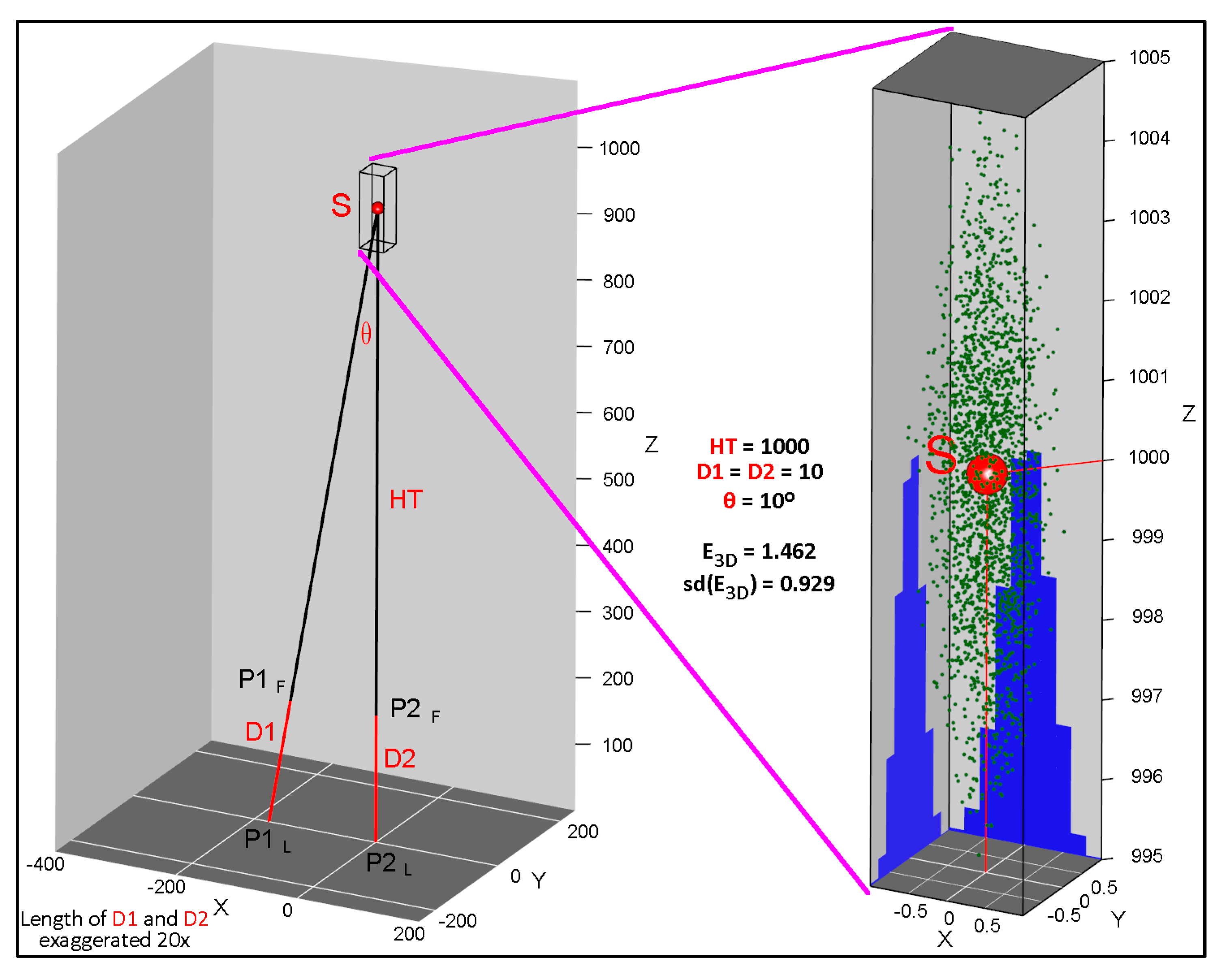
Let two pulses P1 and P2 intersecting at scanner location S that is positioned at height HT above the ground. The coordinates of the last (P1L, P2L) and first returns (P1F, P2F) define the 3D equation of each pulse ray and the distance D between them (Figure 2). P2 is set to be perpendicular to a horizontal plane so that the angle θ it forms with P1 at location S is also the pulse angle of P1. Next, we add noise to the coordinates of P1L, P1F, P2L, and P2F of magnitude that follows the distribution of precision reduction introduced when real numbers are rounded to two decimal digits, the typical level of precision in ALS deliverables. It can be shown that the resulting per-dimension coordinate error term induced by the rounding has range [−0.005, 0.005] and is distributed ~U(0,2.88675*10−3).

Figure 2.
Spatial arrangement of two pulse rays defined by their first (P1F and P2F) and last (P1L, P2L) returns, forming angle θ, and intersecting at S and above-ground height HT (left). The closest points of approach (CPAs) of non-intersecting ray pairs resulting from jittering all four returns are denoted as green dots enveloping the original intersection point (S). The histograms in blue denote CPA distributions along the X and Y axis. E3D denotes the mean 3D distance of CPAs from S (right). Please see text for a detailed description.
With all four return coordinates displayed in Figure 2 jittered from their original position, the two pulse rays no longer intersect at S. We identify on each jittered pulse ray the point that is closest to the jittered instance of the other pulse ray. A third point located exactly on the middle of the line segment that connects these two closest, one on each ray, points is often called the closest point of approach (CPA). It can be computed using calculus [31]. We adopted an alternative, more geometric approach described in [32]. The 3D distance between the CPAs and S (Figure 2) quantifies the effect of return coordinate precision on ray convergence.
We considered 9600 combinations of HT, distance D between first and last return, and pulse angle θ. The values considered for each parameter are displayed along the axes of each panel in Figure 3. For each combination, we run one million coordinate jittering instances, calculating for each the distance of the corresponding CPA to S and the distribution moments of that distance. All computations were performed in R [33] with embedded C code for gains in computational efficiency. The error mean across parameter combinations ranged from 0.092 m to 134.128 m, with median 0.786 m, mean 2.193 m, and standard deviation 5.522 m. We finally regressed the three parameters, HT, D, and θ, after applying a natural log transform to their values, against the natural log of the error means (see Supplementary Materials). The resulting regression formulation was:
with R2 = 0.9942. Equation (1) confirms that the error increases with platform height above the targets and decreases as the distance between pulse returns and the pulse angle increase. It implies that within a set of multi-return pulses of various angles and first to last return distances, we can identify those conducive to a more precise estimate of pulse convergence location and, therefore, of the position of the laser instrument onboard the airborne platform. We provide the code that performs the simulation so that variants of Equation (1) can be calculated for parameter values representative of a specific ALS data set.

Figure 3.
Distribution of 3D error computed using Equation (1) as discrepancy between the location of two intersecting pulses and their closest point of approach calculated after noise is added to the coordinates of returns that define each pulse ray. The error is displayed as function of the above-ground pulse intersection height HT, distance D between the first and last return of each pulse, and angle θ formed between the two originally intersecting pulses. In each of the three panels, one of the three parameters has a fixed value, the other two display their entire value range.
With pulse repetition rates ranging from tens to hundreds of thousands per second and a nominal above-target flight height between hundreds and a few thousand meters, the position of the laser instrument onboard the airborne platform can be considered practically stationary during the time it takes to emit pulses within a single scan line, or, equivalently, a full swing of the oscillating or rotating mirror of the laser instrument. By calculating the ray equations of multi-return pulses from the coordinates of their first and last returns, we can estimate the location of the instrument as the centroid of all CPAs between them. The exhaustive computation of CPAs across all multi-return pulses emitted within a single scan line is logistically infeasible though. Consider, for example, an instrument with 150 kHz pulse repetition frequency, 60 Hz mirror (scan) rate, and ±30 degrees scan angle, operating over a forested landscape. Assume also that, owing to customer-preferences, pulses with absolute scan angle higher than 20 degrees are filtered out prior to delivery. Within 16.7 ms, the time it takes for a full mirror swing, 2500 pulses will be transmitted. After removing one-third of them as exceeding the scan angle specifications and another one-half expected to yield single returns, we are left with 833 multi-return pulses. The pairwise combinations of those 833 pulses are 346,528 per 16.7 ms or 20,791,680 s−1. For a scanning swath generated during 10 min of instrument operation, the pulse combinations are more than 12 billion (1.2475 × 10¹⁰), along with an equal number of CPAs, the calculation of which comes with substantial computational cost. Further, an exhaustive computation will include many near parallel pulse ray pairs that would generate CPAs positioned at larger distances from the actual platform position. According to Equation (1), for HT = 1000 m, D = 10 m, both common settings, and θ = 0.1 degrees (near-parallel pulse rays), the expected CPA error is 72.8 m, a large distance. We have confirmed experimentally that CPA outliers emerging during a single scan swing are not distributed uniformly around the true platform position and thus bias its estimation calculated as the centroid, or other similar metric, across all CPAs for the scan swing in question. We thus adopted an alternative, selective rather than exhaustive approach that identifies specific pulse pairs to use for CPA calculation. The selective approach is computationally efficient.
Raw ALS data are typically delivered organized in tiles of rectangular planar extent. Each tile contains returns from multiple adjacent scan swaths. In our application, the tile files must first be reorganized into individual swaths. We provide a program that supports the reorganization process. Our program assumes the swath identifier is stored in the “point source ID” field in LAS files (see Supplementary Materials) and only works with LAS formats up to version 1.2 [26]. Similar capability is also available in LAStools using the lassplit program. LAStools supports all versions of the LAS format and data compressed using the LAZ format [34]. The scan swaths are then processed sequentially. Each is queried to identify and remove single return pulses and the intermediate returns of multi-return pulses. For the remaining pulses, the 3D distance between the first and last return and the pulse angle are calculated and entered in Equation (1) to generate pulse-specific estimates of the expected error in pulse ray convergence to the actual airborne platform location. The computed estimates are treated as pulse-specific weights. The sign of scan angle pertaining to each pulse, recorded in the raw laser file, is applied to the weight, resulting in positive values towards one side of the swath and negative towards the other. Although the number of weights that must be computed can still be large, approximately 3 × 10⁷ in the 10-min swath given as an example above, it is approximately three orders of magnitude smaller than what it would be required for an exhaustive calculation of CPA across pulse pairs. In addition, the calculations embedded into Equation (1) are a linear scaling of tabular values, namely pulses angle and the distance between first and last return, calculated previously and are thus performed efficiently.
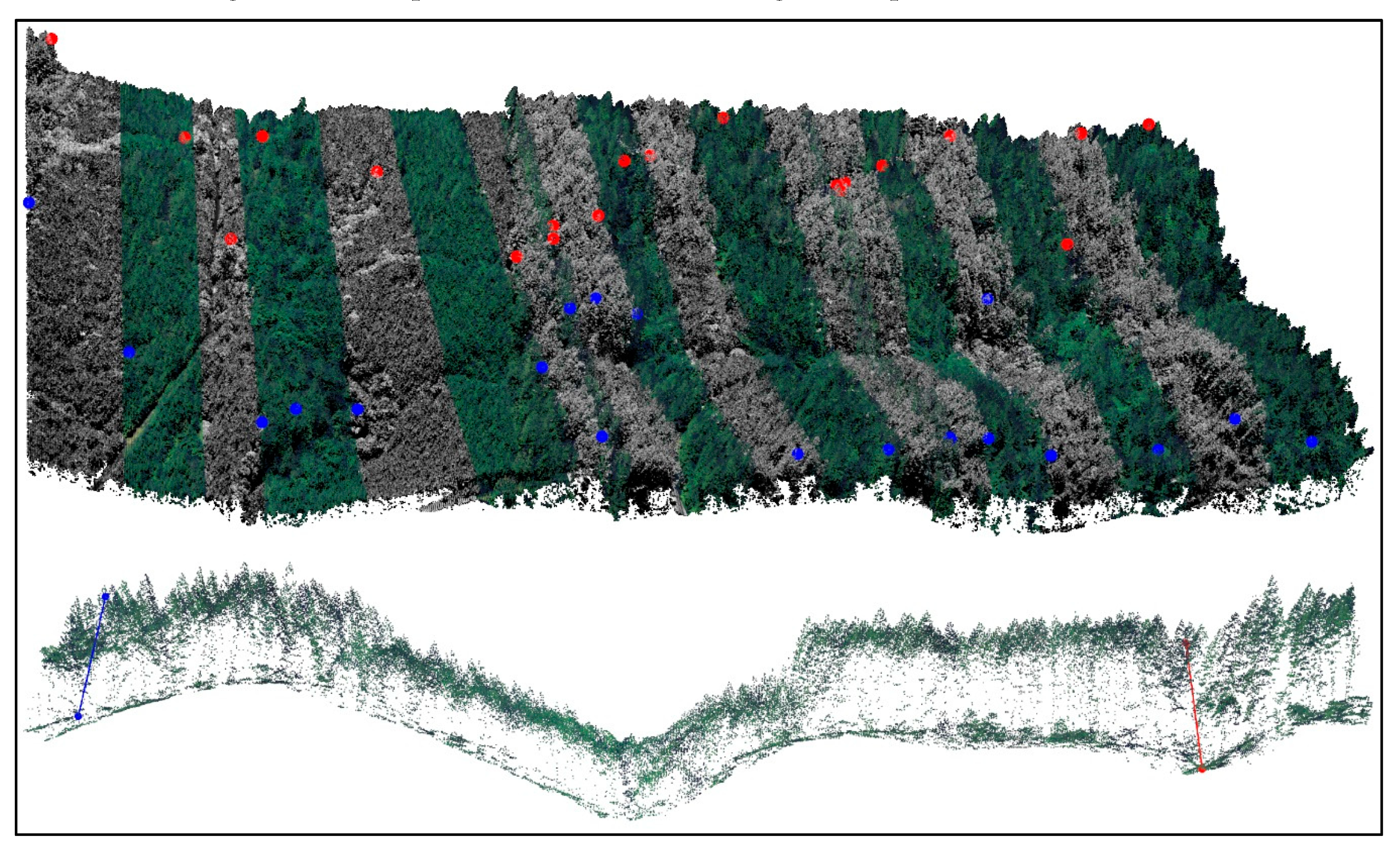
Next, we specify a time interval Δt that must be at least equal or larger than the time it takes to complete a full swing of the laser instrument’s mirror. Δt is used to assign swath pulses into contiguous, in terms of GPS time, groups, henceforth referred to as time blocks. The reciprocal of the scan rate, usually mentioned in data delivery reports, can be used to determine the minimum value of Δt. Then the weights of the pulses in each time block are queried. The two with the extreme values are identified and the CPA of their rays is calculated. Henceforth, they are referred to as the optimal pulses in the time block, in the sense that they their CPA is expected to be the closest among all other pulse pairs of the time block to the actual trajectory of the laser scanner. The top panel of Figure 4 shows an example with the spatial distribution of the first returns of pulses selected for CPA calculation for each time block. The bottom panel details the rays of the two selected pulses within the return cloud of a single time block. The collection of calculated CPAs, one for each time block and each carrying a GPS time reference, represents the trajectory of the airborne platform location for the scan swath.
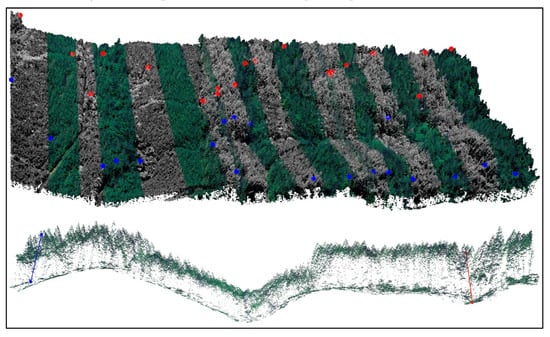
Figure 4.
(Top) Perspective view of an ALS scan swath, showing return membership to 1s time intervals (blocks) colored by alternating intensity (gray-scale) and red-green-blue (RGB) values. Superimposed pairs of red and blue dots, one per time block, show first returns of pulses identified as optimal for determining the platform’s position. The aircraft was moving from right to left. Owing to variability in the speed and attitude of the airborne platform, block width varies. (Bottom) Profile of returns in a time block displayed perpendicular to the airborne platform trajectory, the calculated pair of optimal pulses, and their rays as colored lines. The width of the scan swath is approximately 250 m in both panels.
2.3. Closest Points of Approach (CPAs) to Platform Trajectory
The form of a CPA set calculated for a scan swath using the methodology described above can vary, depending on the characteristics and spatial distribution of the objects illuminated by the laser. In general, CPA sets appear as linear features, and thus conducive to a detailed and precise extraction of the actual airborne platform trajectory via interpolation. A closer inspection, however, often reveals discontinuities, primarily along the Z axis, and noise, sometimes of substantial magnitude. To prevent serious issues with trajectory interpolation, CPA outliers must be removed. We do this using an iterative process that relies on fitting cubic splines [35,36] to each CPA set. We define a vector of distance thresholds sorted in descending order, and CPA points with residuals from the spline fit exceeding the threshold that is effective for the iteration in question are removed. The 3D distance thresholds used in the five study areas were 500, 300, 200, 150, 100, 75, 50, and 25 m respectively. The cubic spline fit in the last iteration becomes the estimated platform trajectory. The formulation of the spline uses the GPS time as an independent variable. For a given time, it provides an estimate of the [X, Y, Z] vector of the laser instrument.
Cubic splines are a specific type of polynomial interpolation techniques. Unlike them, standard methods apply an nth degree polynomial to a set of n + 1 unique values with yi = f(xi), (i = 0, …, n), where xi represents the observed values and yi the interpolation estimates. A major deficiency of these methods is that as the number of observations increases, so does the degree of the polynomial, leading to overfitting and oscillatory polynomial behavior particularly towards the ends of the observed value series. Splines attempt to overcome the overfitting issue by utilizing several, instead of just one, low degree polynomials Pi(x), each fit in the interval between xi-1 and xi. The degree of the polynomials defines the spline type. Cubic splines S(x) utilize third order polynomials with formulation that ensures continuity and smoothness. Continuity implies that any two consecutive polynomials yield the same value estimate, or ‘connect’, at joint value xi, and Pi(xi) = Pi+1(xi). Smoothness requires that they have the same derivative at their joint value, or , where λ is a smoothing parameter. Larger values of λ induce more smoothing. The objective function of a cubic spline is:
where P″ is the second derivative of the polynomial effective at value x. The first component of the objective function represents the typical standard error between observed and predicted values. The second component is known as the smoothing operator and determines the curvature of the spline. If the interpolation is exact, the spline is forced to pass through each of the observed values yi, the standard error component of Equation (2) is zero, and the curvature of the spline could be rather pronounced, mimicking the oscillatory polynomial behavior mentioned earlier, thereby inflating the overall value of the objective function. Conversely, if λ = 0 no smoothing is applied, often leading to a standard error component of large value, especially if the xi values contain substantial amounts of noise. The optimization of the objective function is achieved iteratively, within predefined bounds of λ. Alternatively, the optimization can be applied to a subset of the observed xi values. Given the arrangement of a CPA set in space, the optimization is carried is each dimension separately. We fit cubic splines to all CPA sets using the smooth.spline function in the R stats base package considering the CPA parent pulse weights. The value of parameter λ is implicitly constrained within [−1.5, 1.5].
We investigated systematically the effects time block duration (Δt) and CPA intensity, defined as the time interval between points considered in the cubic spline optimization process detailed above, have on airborne platform trajectory estimates obtained for flight lines in each of the five study areas. We used Δt values from 0.01 s to 0.05 s at 0.01 s intervals and from 0.05 s to 1 s at 0.05 s intervals (total 24) and CPA intensity ranging from 1 point per second to 1 point every 10 s of flight time, at 1 s intervals. A total of 240 cubic splines were calculated for each scan swath. To assess goodness of fit, each spline was compared to the recorded platform trajectory, using the GPS time values present in the latter as reference. Finally, we evaluated how the discrepancies between estimated and observed trajectory lines propagate to the calculation of pulse angles and the relationship between pulse and scan angles recorded in the raw laser data.
3. Results
3.1. Scan Swath Completeness
Nearly one third (32.4%) of the laser scan swaths across the five study areas had a portion missing (Table 3), owing to trimming of the return clouds prior to data delivery to within client requested acquisition boundaries (Figure 5). The ratio was highest in the Deschutes area and the lowest in West Metro. A scan swath was considered trimmed if more than 10% of its planar area was removed by postprocessing prior to data delivery. The trimming sometimes led to two or more discontinuous scan swath parts, as in Figure 5, or removed a section of the swath along one of its sides. Except those with ends perpendicular to the acquisition boundary, all other scan swaths had localized, end-of-swath, trimming. The west end of the swath depicted with red color in Figure 5, shows the effects of the localized trimming, with the swath end truncated to a wedge. For the scan swath depicted in blue color the end trimming is less pronounced. To account for the effects induced by the end-trimming, all scan swaths were processed a second time, after removing 3 seconds of data from either end.

Table 3.
Number of complete vs. spatially trimmed laser scan swaths in each study area. Quantities in parenthesis denote study area percentages.
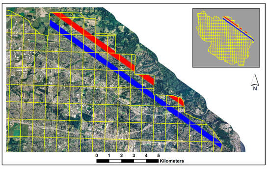
Figure 5.
Example of complete (blue) and trimmed (red) scan swaths in the West Metro area superimposed on panchromatic NAIP imagery. Polygons with yellow outline denote data delivery tiles.
3.2. Spline Fit Evaluation
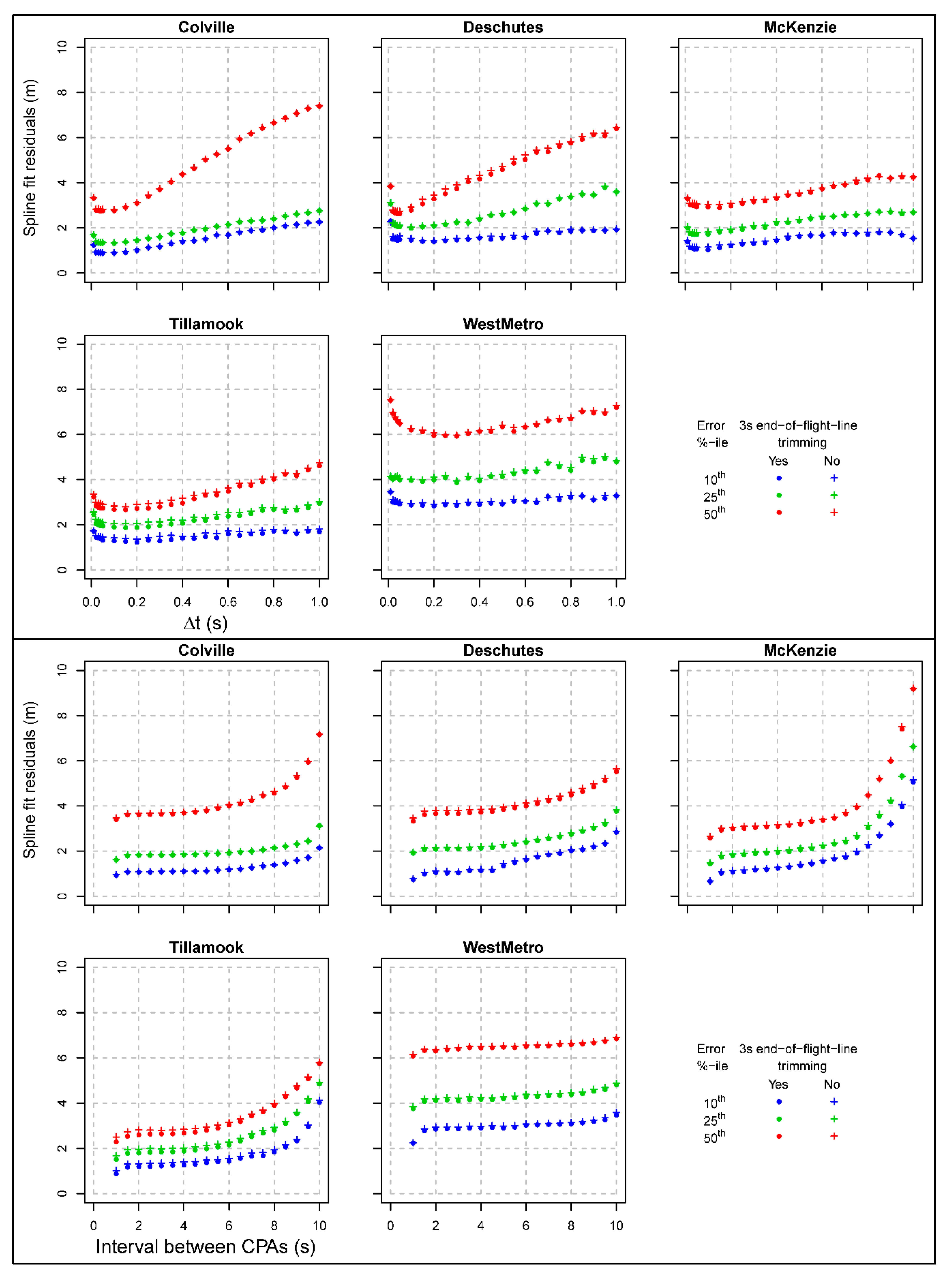
Figure 6 shows the distribution of residuals for the spline fit results to CPAs across the study areas, as a function of time block duration Δt and time interval between CPAs (intensity) respectively. Spline fit is quantified by the magnitude of the residuals. The 10th percentile of fit as function of Δt decreases very slowly across study areas, except for Colville, where it decreases faster. The 25th percentile fit decreases at a higher rate compared to the 10th. The fit improves slightly from the shortest Δt considered (0.1 s) to about 0.5 s, after which it increases again. End-of-swath 3 s trimming does not affect the fit. The best per study area median (50th percentile) fit is approximately 3 m, except for West Metro where is twice as much, 6 m. Spline fit residuals increase monotonically as a function of CPA intensity and their relationship has a sigmoidal form with flex points at 1.5 s and 7 to 9 s. The smallest residual median ranges between 2 and 3.5 m (6 m for West Metro). As with Δt, end-of-swath trimming has little effect.
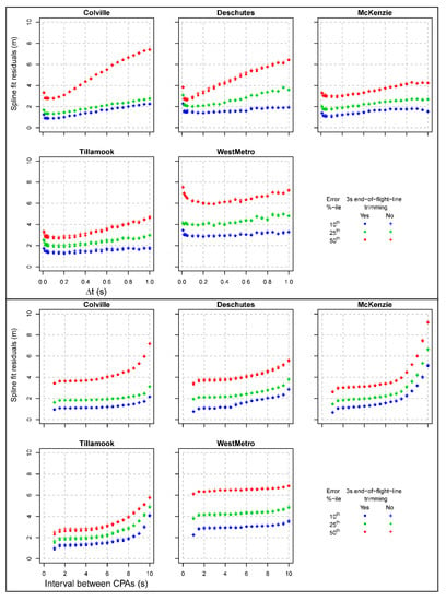
Figure 6.
Distribution of residuals in splines fit to flight-line-specific CPA sets across study areas as function of time block duration (top) and time intervals between CPAs used in the fitting (bottom). Crosses indicate the entire CPA set was used for each flight line; dots denote CPAs trimmed by 3 s on either end.
Results analogous to those presented in Figure 6 are shown in Figure A1 (Appendix A), only this time the swaths are organized into two categories, one with minimal trimming by the acquisition boundary, the other with substantial. The form of spline fit relationship as function of Δt and CPA intensity have remained largely the same as observed previously (Figure 6), but the magnitude of the residual difference between categories varies. The 10th residual percentile across time block duration for Colville shows little difference between trimmed and complete swaths. The 25th percentile for trimmed swaths, however, is 50% higher than for complete ones. The median residual is almost double for trimmed swaths and short Δt, but slowly converges to that observed for complete swaths for higher Δt values. In Deschutes, the trimmed swaths have lower 10th percentile residuals than the complete swaths, as it is also the case, although of much smaller magnitude, in Colville, Tillamook, and West Metro. The sigmoidal relationship of residuals as a function of CPA intensity persists (Figure A1, bottom), and the residual offsets are regular for all percentiles shown, except for the Deschutes area. As with Δt, for shorter time intervals between CPAs, the residual percentiles for complete swaths are higher than for trimmed ones in the Deschutes, and WestMetro areas; the order is reversed for larger time intervals between CPAs.
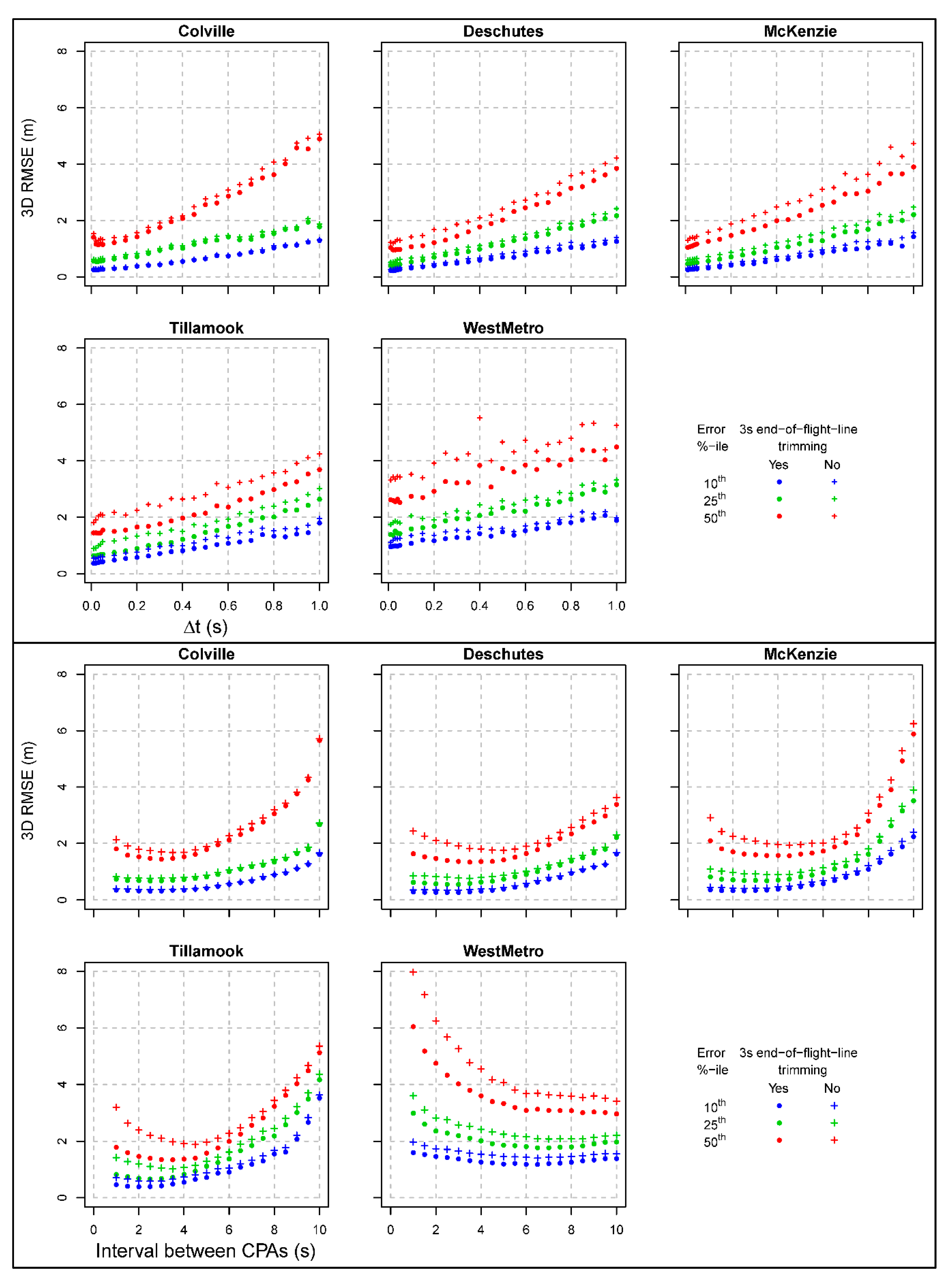
Figure 7 shows the spline fit to recorded laser instrument positions as a function of Δt and CPA intensity, quantified as the root mean square of the 3D distance, or 3D error (RMSE), between estimated and actual positions. It is evident that the magnitude of the error increases practically linearly with Δt across all study areas. End-of-swath trimming reduces the error by a small margin in Tillamook and West Metro, or not at all in Colville, at least for the lower distribution percentiles. The 10th error percentile for Δts shorter than 0.4 s is below 1 m for all study areas and approximately 1 m for West Metro. For the shortest Δt considered (0.1 s) the 10th error percentile is about 30 cm while the median error is under 2 m (under 4 m for West Metro). Examined as a function of CPA intensity (Figure 7, bottom), the form of the error varies. It increases monotonically for lower distribution percentiles, except for West Metro where there is very little variability. End-of-line trimming has practically no effect for lower distribution percentiles and is moderate for higher ones. The median error is lowest for CPA intervals in the 3 to 5 s range, while in West Metro the lowest error median is observed for larger intervals, 6 to 10 s.
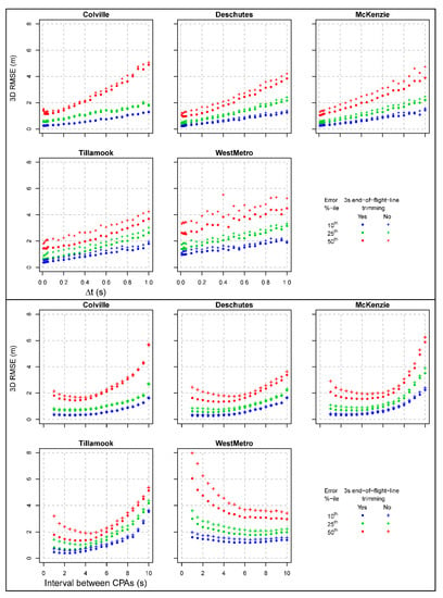
Figure 7.
Distribution of error percentiles in splines fit to flight line-specific CPA sets across study areas as function of time block duration (top) and time intervals between CPAs used in the fitting (bottom), calculated using recorded platform positions. Crosses indicate the entire CPA set was used for each flight line; dots denote CPAs trimmed by 3 s on either end, to reduce effects induced by acquisition boundaries.
The effects of acquisition boundary trimming are shown in Figure A2 (Appendix A). Unlike what was observed for the spline fit to CPA sets, the fit to the actual locations of the laser instrument across Δts is substantially worse for trimmed swaths, especially for higher error distribution percentiles. For most study areas, the median error for trimmed swaths is double that for complete. Note that the Y axis of panels in Figure A2 includes discontinuities aiming at preserving enough detail where the error rates are low, while including the higher error values. For any given error percentile, the error values corresponding to Δt values for trimmed swaths are occasionally rather different than those for neighboring Δts. For example, in the Colville area, the value of the 10th error percentile for Δt = 0.75 s is 3.15 m but only 1.30 m for Δt = 0.70 s. No similar anomalies were observed for complete swaths. The relationship between RMSE and CPA intensity (Figure A2, bottom) is complex. For complete swaths the 10th percentile of error distribution is increasing monotonically but at a low rate, with the rate increasing for larger intervals between CPAs or it is practically stationary (West Metro). For trimmed swaths the 10th error percentile is about 20 cm higher than for complete ones in Colville, 50 cm in McKenzie, and 150 cm in West Metro. In Deschutes, the error metric has the same value for CPA intervals between 4 and 7 s for both complete and trimmed swaths. For higher or lower CPA interval values, the error of the trimmed swaths is higher. In Tillamook, the 10th percentile of the fit error is lower for trimmed than for complete swaths when the CPA intervals exceeds 7 s. For higher RMSE distribution percentiles, the fit is much worse for trimmed swaths than for complete. The maximum median RMSE for trimmed swaths is 8 m in McKenzie (CPA interval is 10 s) and more than 40 m in WestMetro for CPA interval equal to 1s. Across study areas the 25th RMSE percentile for trimmed swaths rivals in magnitude or exceeds the median RMSE for complete swaths.
These findings suggest that for most of the 444 scan swaths examined, shorter time block duration values tend to provide the best spline fit to the actual laser instrument location. The effects of CPA intensity are less clear, however, given that the lowest 25th and 50th RMSE percentile values (best fit) often occur for larger intervals (Figure 7). Based on these observations, we selected a pair of parameter values, Δt = 0.1 s and CPA interval of 4 s, expected to yield near optimal results for most scan swaths, and then examined the corresponding fit values across study areas and swath processing options (Figure 8). For the parameter values selected, the spline fit residuals per study area are robust against swath processing options. Median spline fit residual is lowest for Tillamook and Colville and highest for West Metro. McKenzie exhibits the highest variability. Within each study area, the median residual is the smallest when considering only complete swaths and applying a 3 s trimming on either end, followed by complete swaths with no end-trimming applied.
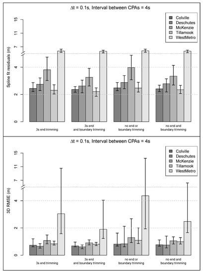
Figure 8.
Distribution of residuals in splines fit to flight-line-specific CPA sets (top) and of spline error calculated using recorded platform positions (bottom) for a selected time block duration and time interval between CPAs. Bars represent the median and the whiskers the 25th and 75% percentile respectively. Note the scale discontinuities along the Y axis.
The residuals are the largest when considering all swaths and applying no end trimming. The residual differences across options for the same study area are very small, ranging from 2 to 15 cm. Note that the maximum range between 25th and 75th percentile for residuals in West Metro across swath processing options is only 27 cm, even though the residual median is 5.20 m. For the rest of the study areas, the error median spline fit residual ranges between 2 and 4 m.
The spline fit error, however, is much lower, 1 m or less, except for West Metro. Unlike the residuals of the spline fit to CPA sets, the fit error (against recorded platform locations) varies more within each study area (Figure 8, bottom). In the Deschutes study area, for instance, the lowest error median is observed for complete swaths with end trimming applied (62 cm), followed by all swaths and end trimming (66 cm). The error range is also the lowest for those options, 29 and 33 cm respectively. When no swath-end trimming is applied, the error range is much larger, 87 cm for complete swaths and no end trimming and 150 cm for all swaths and no trimming. The 25th to 75th percentile error range for West Metro is much larger, up to 11.5 m. As a reminder, the spline fit results shown in Figure 8 are for time block duration and CPA intensity setting believe to yield near optimal results. For other combinations of fitting parameter choices, the error levels are much higher, and the fit metrics calculated are volatile (results not shown).
Figure A3 (Appendix A) illustrates the spline fitting process to a CPA set for a Colville scan swath, with the recorded trajectory of the laser instrument superimposed. The right half of the CPA set corresponds to an area with dense, continuous canopy forest, except the very end which is over water. At the right half there is very little variability in the positioning of the CPAs and the spline matches precisely the recorded trajectory. The left half is over sparse forest and mostly large patches of short vegetation. The CPA set is less compact there, yet there is still close correspondence between the recorded and estimated trajectory. The left end of the swath is trimmed by the acquisition boundary and has fewer multiple-return pulses, on which our process relies, and those represent only one side of the scan swath. The resulting large spacing between CPAs, and the positional noise they contain, leads to a spline fit that deviates substantially from the actual positions. It should be noted that the RMSE values computed for the planar dimensions are much larger than for the vertical dimension. Also, that although the fit of the cubic spline has submeter precision for 85% of the scan swath, the deviations observed near its two ends inflate the overall 3D RMSE value.
As stated in Section 2.2, the weights used to determine the optimal pair of pulses for a given time block, were obtained via simulation which uses the nominal above-target height as a controlling parameter. Table 2 shows the nominal heights retrieved from the vendor data delivery reports. Altering the nominal height changes the pulse pair selected per time block, the ensuing CPAs, and the spline formation and fit. Table 4 shows changes in the mean RMSE calculated using all swaths with 3 s end-trimming for the West Metro and McKenzie study areas. In both study areas, the actual nominal height was the one yielding the lowest (best) RMSE.

Table 4.
Cubic spline fit error against recorded laser instrument positions for selected above ground heights. Height is used to calculate pulse weights that, in turn, determine the selection of time block pulses participating in the formulation of CPAs. The nominal height effective for laser data acquisition in each study area is in bold. All swaths were used in the computations, with 3 s end trimming applied. Spline fit is represented as Root Mean Square Error (RMSE).
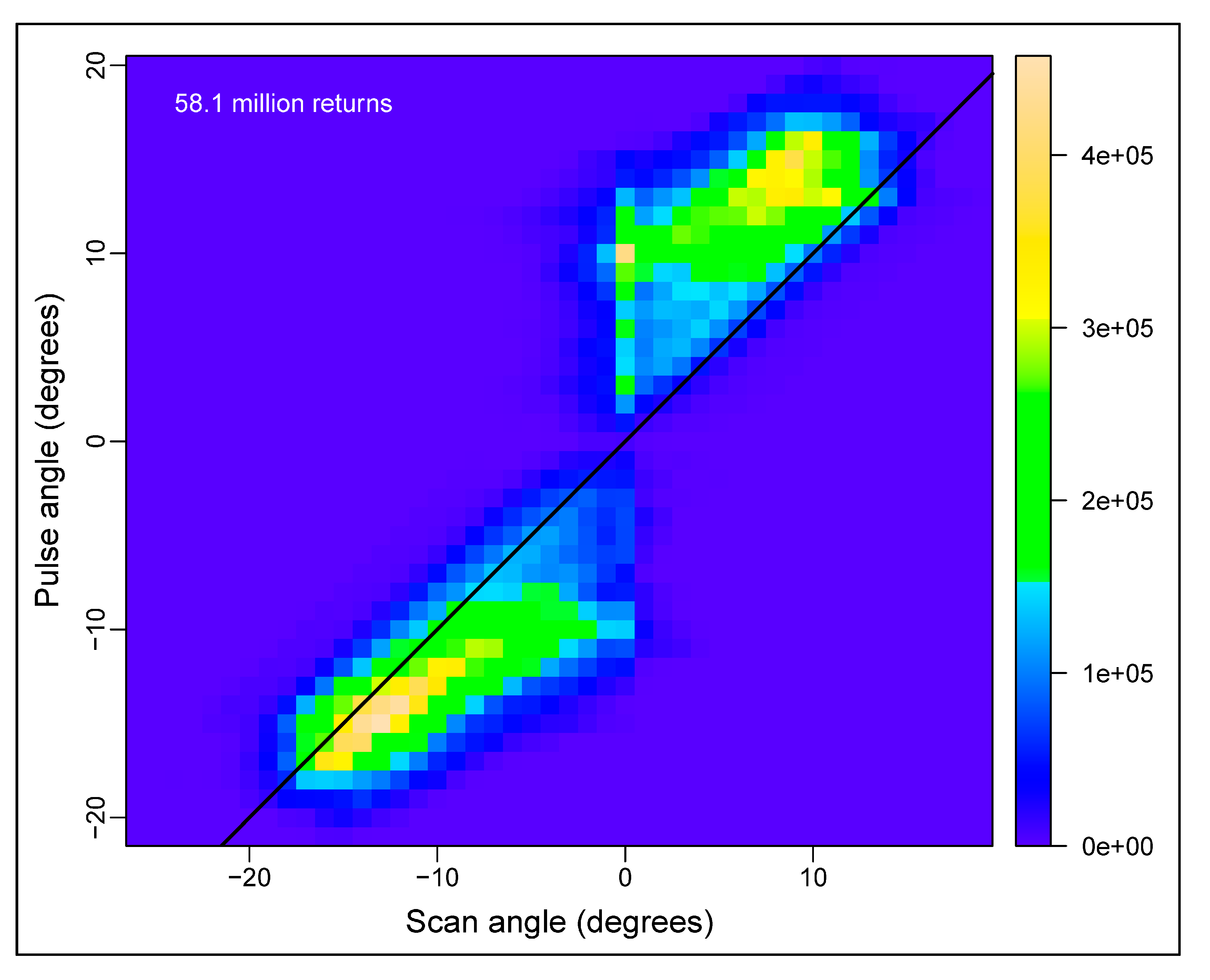
An advantage associated with deriving the laser instrument trajectory from the return cloud, when the actual one is missing from the laser data deliverables, is manifested in Figure A4 (Appendix A). The figure pertains to a Colville area scan swath over steep terrain and shows the discrepancies between the scan angle recorded by the laser instrument and the corresponding pulse angle calculated from the recorded trajectory. For a little over 58 million returns, the angular discrepancy is greater than 5 degrees for 37.7% of them; and greater than 10 degrees for a 6.1%. It suggests that the precision, and likely the accuracy, of analyses that rely on pulse angles can be benefited from their estimates obtained by using the process introduced herein, rather than relying on the recorded scan angles.
4. Discussion
The approach introduced in this study can retrieve the trajectory of an airborne laser instrument by exploiting the spatial arrangement of multiple return pulses it generates. Over forested areas the retrieval is accurate and precise, provided that recommended values for parameters which control the process are applied. In the presence of continuous canopies, time block duration under 0.5 s, and time interval between CPAs not exceeding 5 s, submeter precision should be expected (Figure 7). In such conditions, the estimated trajectory obtained by using our approach should be considered practically equivalent to the actual trajectory with a degree of precision adequate for most uses. The error rates observed over forested areas ensure that efforts to calibrate the raw recorded return intensity using the range (distance) and angle between the instrument and individual returns will require adjustments that are no more than 1 unit, for intensity quantified in the 0–255 range, different from those obtained by using the actual trajectory. Differences between estimated and recorded pulse angles will not exceed a few mrad. Even with suboptimal parametric choices, the trajectory estimation error should be expected to not exceed a few meters. The observed performance was achieved by applying our approach to dense return clouds (>7.5 pulses m−2). For optimal performance in acquisitions with much lower pulse densities, time block duration and CPA interval might need to be adjusted.
Our methodology partitions individual scan swaths into continuous, non-overlapping sections (time blocks), and for each section it identifies the pair of pulses believed to be optimal for assessing the position of the laser scanner. These provisions reduce the overall computation load and expedite the process. Our approach performs best where multi-return pulses are present in all time blocks and swath parts. Sporadic departures from this ideal arrangement are usually tolerated quite well (Figure A3). Where, however, there is a paucity of multiple return pulses across several consecutive time blocks or where the multi-return pulses are concentrated in a specific part of the swath, performance is suboptimal and the estimation error higher. Agricultural land and urban areas with limited tree cover belong to this category. Both discrete and waveform laser data sets restrict identified returns to be no closer than a threshold distance along the pulse trajectory. In the five study areas this threshold was between 1.5 and 2 m. The implication is that vegetation shorter than the threshold, the usual case over agricultural crops, will be represented only by single return pulses that are removed in an early stage of our process because they do not permit the calculation of the pulse’s ray. In urban areas, the majority of targets are opaque to the pulse photons and yield only one return. Buildings often completely occlude trees and tall plants or limit their exposure to the scanning instrument from limited viewing directions. Similarly, pulses with multiple returns from building sides and other manmade structures are concentrated to a narrow strip underneath the airborne platform where their angles to the vertical are narrow. In such conditions, and as implied by Equation (1), the CPAs generated can have large location errors. This is manifested in the West Metro area where the estimation errors are much larger than all the other study areas. Results from the same area suggest that in the presence of lower density and lack of uniformity in the spatial distribution of multiple returns, the value of the CPA interval parameter should be higher than those over forested areas.
We explored many alternatives and scenarios aiming at improving the scanner trajectory estimation for scan swaths containing large areas with few multiple returns or with multiple return pulses concentrated to a particular section but were unable to identify a consistent solution for those challenging circumstances. The alternatives explored included, but were not limited to, conditioning the directional vectors of the estimated trajectory to parallel the ground surface, locally replacing the cubic with a linear spline, or using dynamic, instead of fixed, time block duration adjusted to the spatial distribution of multi-return pulses. Each of these alternatives was found to improve the estimation precision for a selected subset of swaths but reduced it in most others. The approach detailed here had the most consistent performance.
At the design phase of an ALS acquisition, flight lines are drafted to minimize flight time and, therefore, cost. Longer flight lines are usually preferred (Figure 1), often positioned in approximate alignment to physiographic features such as watersheds. The exact spatial extent of data deliverables in the US pacific northwest, however, is often determined by land ownership (Figure 5). The resulting trimming of the return clouds usually affects several swaths proximal to the acquisition boundary and thus our ability to retrieve the scanner trajectory precisely. Trimming along the side of the swath leads to much higher error levels than trimming at the ends. Post-trimming pulses tend to be concentrated to smaller sections of the original swath and their converging rays form acute angles. The simulation results mentioned in Section 2.2 suggest that in such conditions calculated CPAs carry much higher positional uncertainty compared to those of complete swaths. Our analyses with actual data have corroborated this assumption. The acute angle formed between a pair of pulses identified as optimal within a time block, coupled with return coordinates rounding to two digits, occasionally yield CPAs that are kilometers higher than the true position of the laser instrument. At other times, the CPA of a pulse pair is below ground! The iterative fitting of cubic splines is very effective in eliminating outlier CPAs, but it also removes a few legitimate ones, especially where the airborne platform pitch changes rapidly, an event that occurs quite frequently over mountains with alternating ridges and valleys. To quantify the swath trimming effects, we presented our results separately for pulses with and without substantial boundary trimming and/or end trimming. The metric used (3D RMSE) to evaluate performance is the standard applied to performance assessments of models that have spatial components. It is, however, sensitive to outliers. As documented in Figure A3, trajectory estimation errors corresponding to a small part of the swath processed, even for a few seconds on either of its ends, inflate the overall error. To mitigate this sensitivity, we used percentiles as metrics of 3D RMSE distribution in our presentation of analysis results.
An analyst applying our methodology can only evaluate the residuals of the spline fit to CPAs (Figure 6 and Figure A1) as indicator of method performance. A typical residual median should be expected to be in the 2 to 4 m range over forested areas, and perhaps twice as large elsewhere (Figure 8). Our results indicate that the actual trajectory estimation error (3D RMSE) would likely be much smaller, about one fourth of the spline fit residual median over forests, and half elsewhere. Although not common, and despite efforts to avoid it, the residuals of the spline fit to CPAs can be zero. This implies an exact fit, with the spline intersecting every CPA, and that the value of the smoothing parameter λ in Equation (2) is near the bounds specified, [−1.5, 1.5] in our analyses. In such occurrences, the sinuosity of the spline is pronounced and the trajectory estimation error large. It is suggested that for the rare cases of swaths with exact spline fit and zero residuals, the time block duration (Δt) and/or the CPA intensity settings are altered slightly and the fitting process is repeated.
Our process was designed to be fully automated so that it can be applied effortlessly to acquisitions of any size. Manual adjustments of Δt and CPA interval coupled with visual assessment of the cubic spline fit will likely improve the trajectory estimation precision for most swaths with the problematic multiple-return pulse distribution characteristics mentioned above. Manual adjustments can also improve the estimation precision for swaths trimmed with the acquisition boundary. For example, the trimmed swath depicted in red in Figure 4 can be split into three sections. While the split will not improve the spline fit of the two shorter sections, it will reduce by more than half the 3D RMSE for the longer, as compared to the error for the entire swath, before the split. Manual interventions by an analyst may be realistic for a data set comprising a small number of swaths. For larger acquisitions, however, as the five used in this study, data processing involving multiple iterations and substantial analyst involvement can be economically and logistically infeasible.
The implementation of our approach requires two passes over the raw return cloud files, one to reorganize the tiled data into swaths, and a second for the derivation of the scanner’s trajectory. Reorganizing the tiled data into swaths is a simple, fully automated task if each return is furnished with a unique flight identifier. Alternatively, the GPS time data can be used to identify swaths, but the process can be complicated if time is recorded in the standard format and the acquisition has lasted more than a week. In such cases, different swaths can have overlapping time intervals and spatial extents. In rare cases, the reorganization process may require several passes over the data and analyst’s supervision. While tile size is controlled by the data vendor to a manageable size, files generated from the reorganization into individual swaths can be very large. In this study, there were many swaths more than 40 km long, with compressed file size [34] larger than 3GB. Processing of very long swaths may necessitate the use of computers with compatible hardware configuration (enough memory). Otherwise the long swath must be first split into chunks with a few seconds of time overlap, followed by processing of each chunk separately to identify time blocks and to calculate CPAs, and finally fuse the chunk CPAs, prior to fitting the cubic spline.
In the event that the nominal above-target height of the scanner cannot be established from the data delivery report or otherwise, a tentative value can be used to compute the vertical distance between the derived platform trajectory and the corresponding terrain elevation for a subset of the scan swaths. The resulting approximate mean above-target height can then be used with the entire data set. As documented in Table 4, discrepancies between actual and approximate nominal heights have limited impact on the overall precision of the estimated scanner trajectory. Achieving the highest attainable precision would require the process to be repeated twice. Once following the standard approach to calculate an initial trajectory, and a second time using time block-specific scanner heights calculated as the vertical difference between individual returns and the initial trajectory. The extra effort may be warranted in data acquisitions over mountainous terrain where departures from the nominal above-target height can be frequent and substantial.
The coefficients of pulse angle and distance between first and last return are used as weights to determine the pair of pulses present in a time block that is optimal for assessing the location of the laser scanner. They can be computed via simulation for a range of pulse angles and nominal scanner height above the target. The code provided for this purpose assumes that the only source of imprecision in the coordinates of returns is rounding to two decimal points. However, return coordinates stored with limited decimal precision in an intermediate system favored by the data vendor and reprojected, using the same level of precision, to the coordinate system requested by the client just prior to delivery carry positional uncertainty that is not anticipated by the code provided. The simulation settings must be adjusted to account for reprojection conditions, before being used to calculate pulse weights.
It is often stated that the scan angle recorded per individual return in raw laser files (see Supplementary Materials) is an adequate surrogate of the pulse angle for analyses that require the latter. Our calculations in each of the five study areas did not support this claim. As shown in the example of Figure A4, a considerable portion of returns exhibited substantial discrepancies between scan and pulse angle. After examining thousands of kilometers or recorded scanner trajectories in the US Pacific Northwest, we determined that these discrepancies emerge primarily from instability in the airborne platform’s pitch. Roll was much more stable. All aircraft used for laser data acquisition in our study areas maintained an upward pitch of about −5 degrees (electronic supplement). This is necessary to ensure adequate air lift. As a result, pulses are nominally directed forward instead of nadir. Larger discrepancies between pulse and scan angles are observed where the airborne platform dives or climbs abruptly, in response to local atmospheric instability or in an attempt to maintain nearly constant distance to the targets, especially over mountainous terrain. It should be noted that for gyrostabilized laser instruments, scan and pulse angular difference are expected to be minimal.
The technique described can be applied to data acquired with unmanned aerial systems (UAS), provided that they fly in approximately linear trajectories, can record at least two returns per pulse, and have return GPS time recorded with precision conducive to identifying individual pulses. Calculated UAS trajectories may be more precise than those computed from airborne systems because their above-target height is much lower and return coordinates are typically recorded with 3 digits of precision. Unlike UAS-based laser data, return clouds from Geiger mode or photon-counting systems are incompatible with our approach owing to fundamentally different data organization in a cubical tessellation with each ‘return’ representing backscattered photons from more than one pulse.
5. Conclusions
The goal of this study was to develop and present a new method that computes the trajectory of the aircraft and thus the laser instrument using the point cloud. Our method is robust and produces trajectories that compare well to those recorded as part of the original data collection effort. While error varies by acquisition, the error in the computed aircraft position seldom exceeded a few meters. In general, the resulting trajectories are sufficient for all applications requiring them. However, success of the method relies on data where pulses have at least two returns. Our main area of interest is in forested areas where the vegetation height and gaps in the canopy between trees, between branches on the same tree, or between leaves or needles result in multiple returns for a substantial proportion of the laser pulses. Our method may not work well with data collected for areas with little or no vegetation.
At first glance, reconstruction of aircraft trajectories may seem like a trivial exercise given that aircraft position data are an essential part of the data collected during an ALS campaign. However, because trajectory data are not typically needed for analyses involving the terrain surface or point cloud, they are often not included as a deliverable. Once the need for the trajectory data is realized, often months or years after the data have been delivered, it may be costly or impossible to obtain. Our work aims to facilitate analyses of ALS data that, for whatever reason, do not include trajectory information.
Supplementary Materials
Supplementary materials are available online at https://www.mdpi.com/2072-4292/11/19/2258/s1. C program LAS_Tile2Swath.exe: Rearranges tiled ALS data to swaths. Supports LAS versions up to 1.2. R program cmp_trj.R: Implements the methodology described in the text. R program cmp_trj_functions.R: includes functions used by cmp_trj.R. 64-bit C library cmp_trj.dll: contains functions called by cmp_trj.R. Please contact the authors if you need a 32-bit version. R program calc_pulse_weights.R: implements the simulation described in the text to compute pulse weights that are required by cmp_trj.R. Video ALS_platform_pitch_and_roll_demo.mp4: real time animation based on actual smoothed best estimate of trajectory (SBET) and ALS data. Documents variability in airborne platform pitch which induces substantial discrepancies between scan and view pulse angles.
Author Contributions
Conceptualization, D.G.; Methodology, D.G and R.J.M.; Software, D.G.; Validation, D.G. and R.J.M.; Formal Analysis, D.G.; Investigation, D.G; Resources, D.G and R.J.M.; Data Curation, D.G. and R.J.M.; Writing—Original Draft Preparation, D.G.; Writing—Review & Editing, D.G. and R.J.M.; Visualization, D.G.
Funding
This research received no external funding.
Acknowledgments
The authors would like to thank Quantum Spatial for help with resolving data consistency issues in one of the acquisitions.
Conflicts of Interest
The authors declare no conflict of interest.
Appendix A
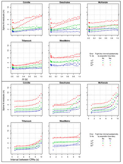
Figure A1.
Distribution of residuals in splines fit to flight line-specific CPA sets across study areas as function of time block duration (top) and time intervals between CPAs used in the fitting (bottom). Dots/Xs pertain to CPA sets from scan swaths free of/affected by substantial trimming with acquisition boundaries respectfully. Note scale discontinuities along the Y axes.
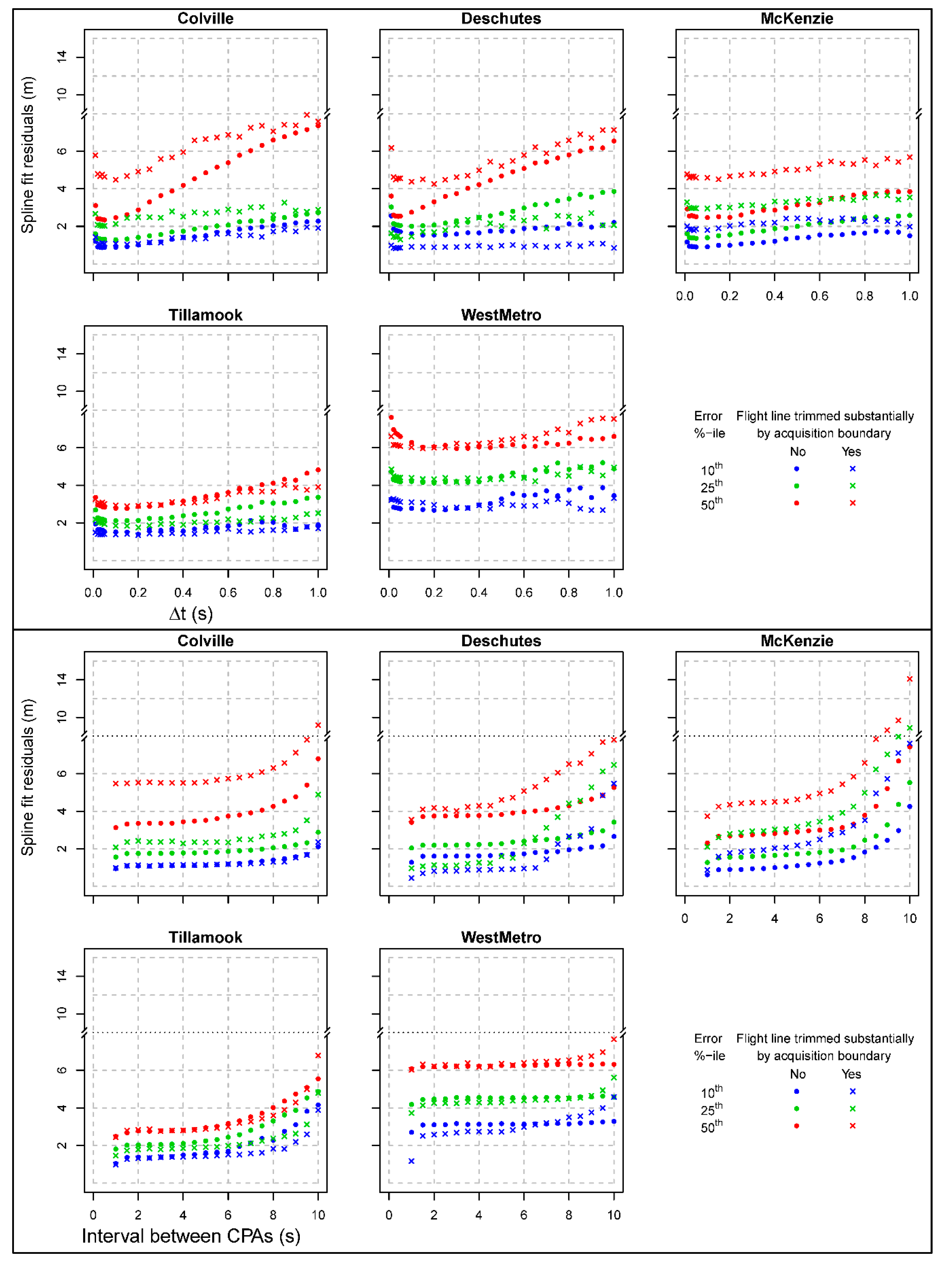
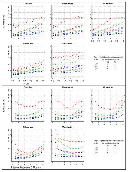
Figure A2.
Distribution of error percentiles in splines fit to flight line-specific CPA sets across study areas as function of time block duration (top) and time intervals between CPAs used in the fitting (bottom), calculated using recorded platform positions. Dots/Xs pertain to CPA sets from scan swaths free of/affected by substantial trimming with acquisition boundaries respectfully. Note scale discontinuities along the Y axes.
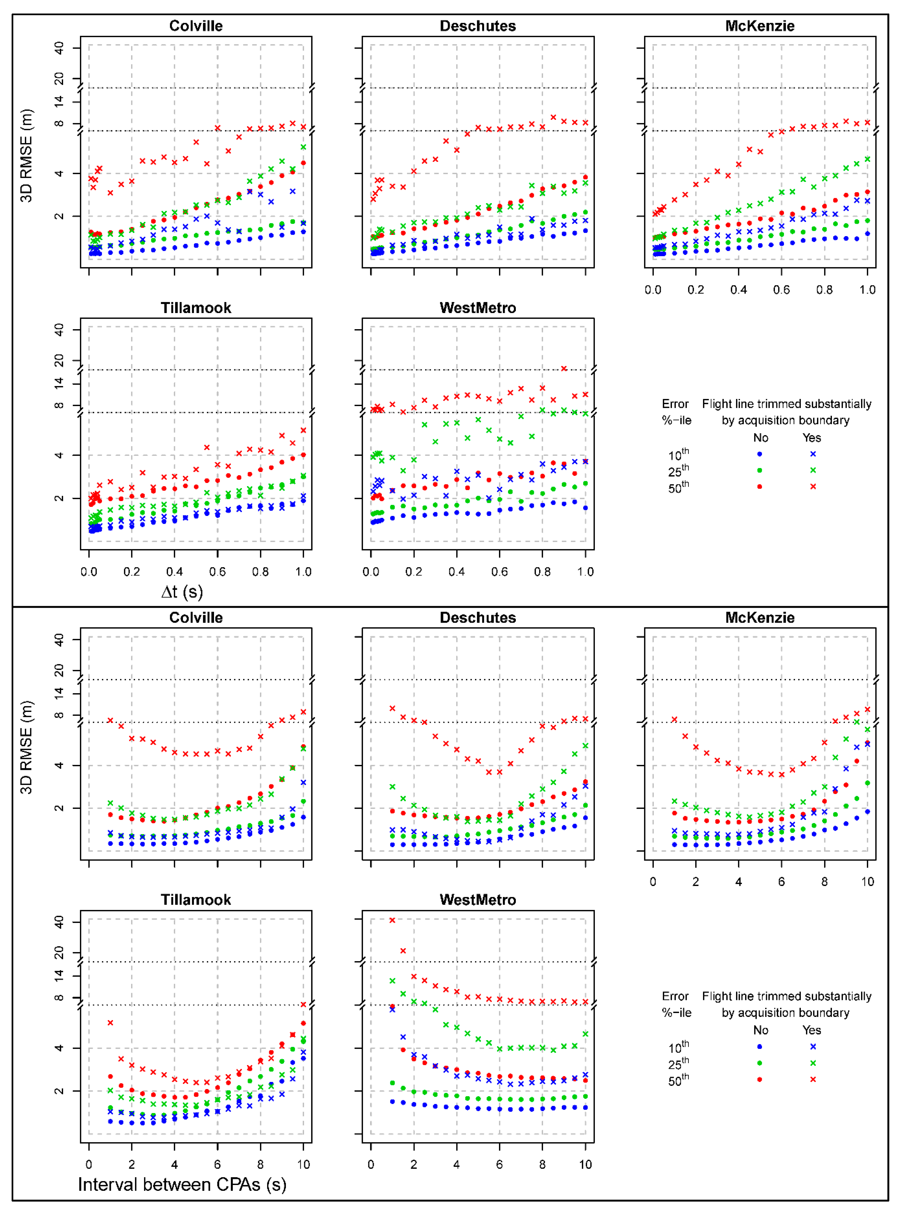
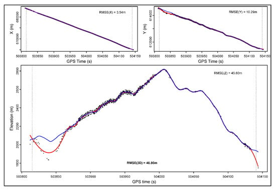
Figure A3.
Example of spline fitting (red line) to a CPA set (points) and the recorded laser instrument trajectory, with each dimension present separately. The Z dimension is featured in larger scale to convey fit detail.
Figure A3.
Example of spline fitting (red line) to a CPA set (points) and the recorded laser instrument trajectory, with each dimension present separately. The Z dimension is featured in larger scale to convey fit detail.
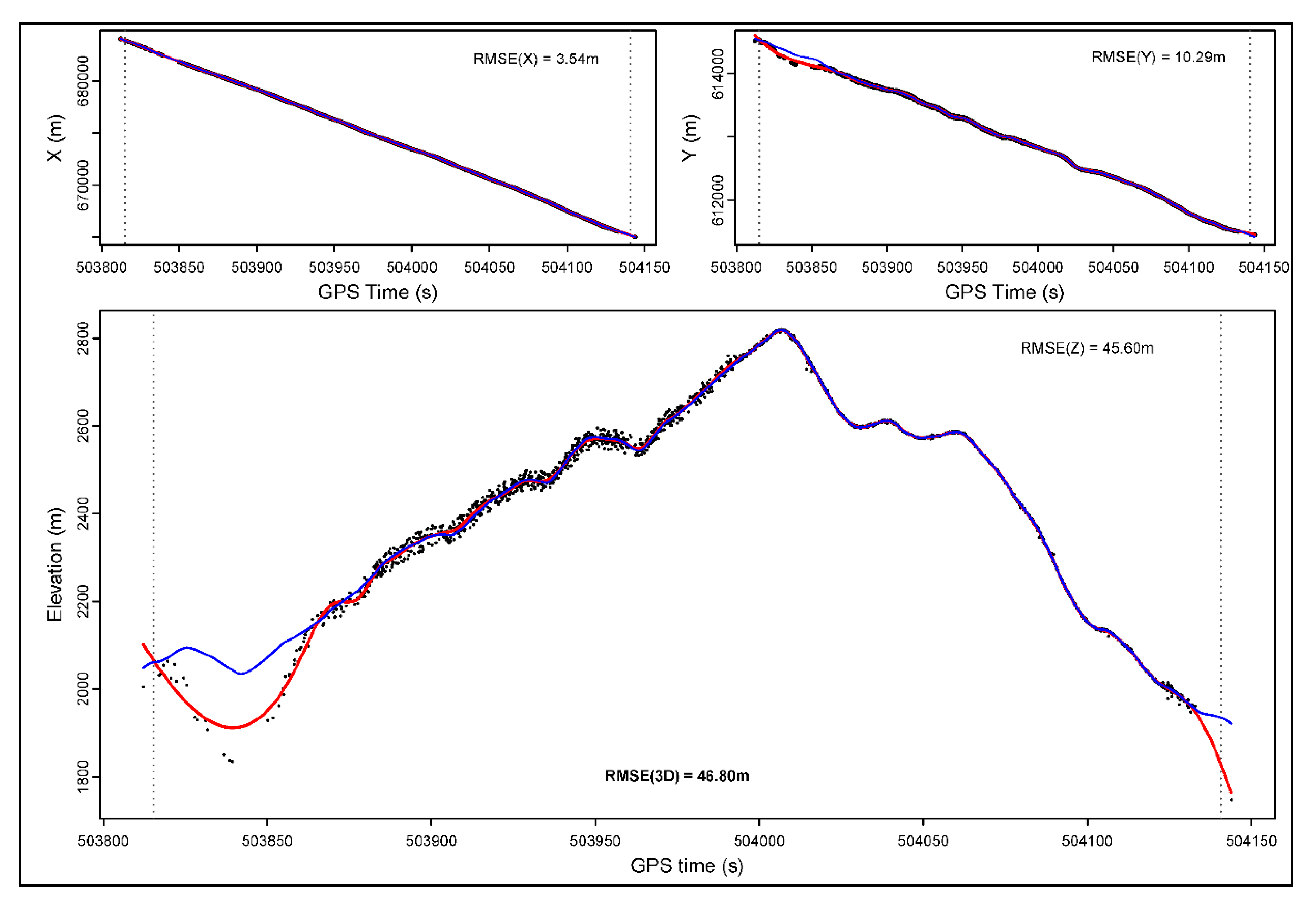
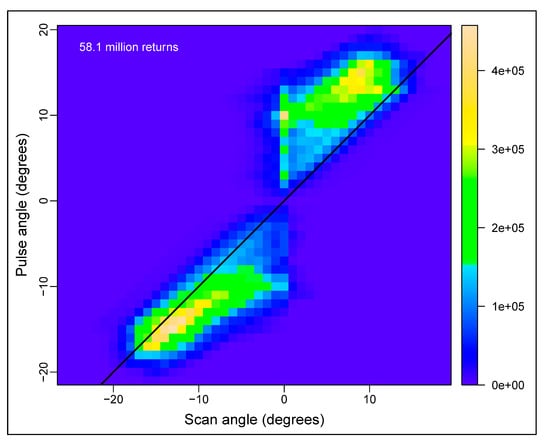
Figure A4.
Two-dimensional histogram of a scan swath from the Colville area, depicting correspondence between recorded pulse scan angle and computed pulse angle. 1:1 line in black.
Figure A4.
Two-dimensional histogram of a scan swath from the Colville area, depicting correspondence between recorded pulse scan angle and computed pulse angle. 1:1 line in black.
References
- Næsset, E. Airborne laser scanning as a method in operational forest inventory: Status and accuracy assessments accomplished in Scandinavia. Scand. J. Forest Res. 2007, 22, 433–442. [Google Scholar] [CrossRef]
- Liu, X. Airborne LiDAR for DEM generation: Some critical issues. Prog. Phys. Geog. 2008, 32, 31–49. [Google Scholar] [CrossRef]
- Barber, C.; Shortridge, A. LiDAR elevation data for surface hydrologic modeling: Resolution and representation issues. Cartogr. Geogr. Inf. Sci. 2005, 32, 401–410. [Google Scholar] [CrossRef]
- Sheridan, R.D.; Popescu, S.C.; Gatziolis, D.; Morgan, C.L.S.; Ku, N.-W. Modeling forest aboveground biomass and volume using airborne LiDAR metrics and forest inventory and analysis data in the Pacific Northwest. Remote Sens. 2015, 7, 229–255. [Google Scholar] [CrossRef]
- Deems, J.S.; Painter, T.H.; Finnegan, D.C. Lidar measurement of snow depth: A review. J. Glaciol. 2013, 59, 467–479. [Google Scholar] [CrossRef]
- Jwa, Y.; Sohn, G.; Kim, H.B. Automatic 3D powerline reconstruction using airborne LiDAR data. In Proceedings of the Laser Scanning, Paris, France, 1–2 September 2009; Bretar, F., Pierrot-Deseilligny, M., Vosselman, G., Eds.; IAPRS: Paris, France, 2009; pp. 105–110. [Google Scholar]
- Huallpa, L.A.M.; Yamazaki, F.; Liu, W.; Chiba, T. Calculation of coseismic displacement from lidar data in the 2016 Kumamoto, Japan, earthquake. Nat. Hazards Earth Sys. 2017, 17, 143–156. [Google Scholar] [CrossRef]
- Soilán, M.; Truong-Hong, L.; Riveiro, B.; Laefer, D. Automatic extraction of road features in urban environments using dense ALS data. Int. J. Appl. Earth Obs. 2018, 64, 226–236. [Google Scholar] [CrossRef]
- Weng, Q. Remote sensing of impervious surfaces in the urban areas: Requirements, methods, and trends. Remote Sens. Environ. 2012, 117, 34–49. [Google Scholar] [CrossRef]
- Goodwin, N.R.; Coops, N.C.; Tooke, T.R.; Christen, A.; Voogt, J.A. Characterizing urban surface cover and structure with airborne lidar technology. Can. J. Remote Sens. 2009, 35, 297–309. [Google Scholar] [CrossRef]
- Höfle, B.; Hollaus, M.; Hagenauer, J. Urban vegetation detection using radiometrically calibrated small-footprint full-waveform airborne LiDAR data. ISPRS J. Photogramm. 2012, 67, 134–147. [Google Scholar] [CrossRef]
- He, C.; Convertino, M.; Feng, Z.; Zhang, S. Using LiDAR data to measure the 3D green biomass of Beijing urban forest in China. PLoS ONE 2013, 8, e75920. [Google Scholar] [CrossRef] [PubMed]
- Alonzo, M.; Bookhagen, B.; McFadden, J.P.; Sun, A.; Roberts, D.A. Mapping urban forest leaf area index with airborne lidar using penetration metrics and allometry. Remote Sens. Environ. 2015, 162, 141–153. [Google Scholar] [CrossRef]
- Rahman, M.T.; Rashed, T. Urban tree damage estimation using airborne laser scanner data and geographic information systems: An example from 2007 Oklahoma ice storm. Urban For. Urban Green. 2015, 14, 562–572. [Google Scholar] [CrossRef]
- Jochem, A.; Höfle, B.; Rutzinger, M.; Pfeifer, N. Automatic roof plane detection and analysis in airborne lidar point clouds for solar potential assessment. Sensors 2009, 9, 5241–5262. [Google Scholar] [CrossRef] [PubMed]
- Santos, T.; Gomes, N.; Freire, S.; Brito, M.C.; Santos, L.; Tenedório, J.A. Applications of solar mapping in the urban environment. Appl. Geogr. 2014, 51, 48–57. [Google Scholar] [CrossRef]
- Korpela, I.; Ørka, H.O.; Hyyppä, J.; Heikkinen, V.; Tokola, T. Range and AGC normalization in airborne discrete-return LiDAR intensity data for forest canopies. ISPRS J. Photogramm. 2010, 65, 369–379. [Google Scholar] [CrossRef]
- Gatziolis, D. Dynamic range-based intensity normalization for airborne, discrete return LiDAR data of forest canopies. Photogramm. Eng. Remote Sens. 2011, 77, 251–259. [Google Scholar] [CrossRef]
- Yoga, S.; Bégin, J.; St-Onge, B.; Gatziolis, D. Lidar and multispectral imagery classifications of Balsam fir tree status for accurate predictions of merchantable volume. Forests 2017, 8, 253. [Google Scholar] [CrossRef]
- Zhao, K.; Popescu, S.C. Lidar-based mapping of leaf area index and its use for validating GLOBCARBON satellite LAI product in a temperate forest of the southern USA. Remote Sens. Environ. 2009, 113, 1628–1645. [Google Scholar] [CrossRef]
- Holmgren, J.; Nilsson, M.; Olsson, H. Simulating the effects of lidar scanning angle for estimation of mean tree height and canopy closure. Can. J. Remote Sens. 2003, 623–632. [Google Scholar] [CrossRef]
- Morsdorf, F.; Frey, O.; Meier, E.; Itten, K.I.; Allgöwer, B. Assessment of the influence of flying altitude and scan angle on biophysical vegetation products derived from airborne laser scanning. Int. J. Remote Sens. 2008, 29, 1387–1406. [Google Scholar] [CrossRef]
- Hopkinson, C.; Chasmer, L. Testing LiDAR models of fractional cover across multiple forest ecozones. Remote Sens. Environ. 2009, 113, 275–288. [Google Scholar] [CrossRef]
- Korhonen, L.; Korpela, I.; Heiskanen, J.; Maltamo, M. Airborne discrete-return LIDAR data in the estimation of vertical canopy cover, angular canopy closure and leaf area index. Remote Sens. Environ. 2011, 115, 1065–1080. [Google Scholar] [CrossRef]
- American Society for Photogrammetry and Remote Sensing. LIDAR Data Exchange Format Standard, Version 1.0, 9 May 2003. Available online: https://www.asprs.org/wp-content/uploads/2010/12/asprs_las (accessed on 31 July 2019).
- American Society for Photogrammetry and Remote Sensing. LAS Specification Version 1.4—R13, 15 July 2013. Available online: https://www.asprs.org/wp-content/uploads/2010/12/LAS_1_4_r13.pdf (accessed on 31 July 2019).
- Gatziolis, D.; Andersen, H.-E. A Guide to LIDAR Data Acquisition and Processing for the Forests of the Pacific Northwest; General Technical Report PNW-GTR-768; US Department of Agriculture, Forest Service, Pacific Northwest Research Station: Portland, OR, USA, 2008; 32p.
- Archuleta, C.M.; Constance, E.W.; Arundel, S.T.; Lowe, A.J.; Mantey, K.S.; Phillips, L.A. The National Map Seamless Digital Elevation Model Specifications: U.S. Geological Survey Techniques and Methods; US Geological Survey: Reston, VA, USA, 2017; 39p. [CrossRef]
- Clarke, S.E.; Bryce, S.A. Hierarchical Subdivisions of the Columbia Plateau & Blue Mountains Ecoregions, Oregon & Washington; General Technical Report PNW-GTR-395; US Department of Agriculture, Forest Service, Pacific Northwest Research Station: Portland, OR, USA, 1997; 114p.
- Blue Marble Geographics. GlobalMapper 20 LiDAR Module. Available online: http://bluemarblegeo.com (accessed on 31 July 2019).
- Eberly, D.H. 3D Game Engine Design; Elsevier: Amsterdam, The Netherlands, 2007; 1040p, ISBN 9780080917993. [Google Scholar] [CrossRef]
- Sunday, D. Distance between 3D Lines & Segments. Available online: http://geomalgorithms.com/a07-_distance.html (accessed on 31 July 2019).
- R Core Team. R: A Language and Environment for Statistical Computing; R Foundation for Statistical Computing: Vienna, Austria, 2016; Available online: https://www.R-project.org/ (accessed on 31 July 2019).
- Isenburg, M. LA Stools—Efficient Tools for LiDAR Processing. Available online: http://lastools.org (accessed on 31 July 2019).
- Hastie, T.J.; Tibshirani, R.J. Generalized Additive Models, 1st ed.; CRC: Boca Raton, FL, USA, 1990; 352p, ISBN 9780412343902. [Google Scholar]
- Chambers, J.M.; Hastie, T.J. Statistical Models; CRC: Boca Raton, FL, USA, 1992; 624p, ISBN 9780412830402. [Google Scholar]
© 2019 by the authors. Licensee MDPI, Basel, Switzerland. This article is an open access article distributed under the terms and conditions of the Creative Commons Attribution (CC BY) license (http://creativecommons.org/licenses/by/4.0/).


