Abstract
Multi-temporal interferometric synthetic aperture radar (MT-InSAR) can be applied to monitor the structural health of infrastructure such as railways, bridges, and highways. However, for the successful interpretation of the observed deformation within a structure, or between structures, it is imperative to associate a radar scatterer unambiguously with an actual physical object. Unfortunately, the limited positioning accuracy of the radar scatterers hampers this attribution, which limits the applicability of MT-InSAR. In this study, we propose an approach for health monitoring of railway system combining MT-InSAR and LiDAR (laser scanning) data. An amplitude-augmented interferometric processing approach is applied to extract continuously coherent scatterers (CCS) and temporary coherent scatterers (TCS), and estimate the parameters of interest. Based on the 3D confidence ellipsoid and a decorrelation transformation, all radar scatterers are linked to points in the point cloud and their coordinates are corrected as well. Additionally, several quality metrics defined using both the covariance matrix and the radar geometry are introduced to evaluate the results. Experimental results show that most radar scatterers match well with laser points and that LiDAR data are valuable as auxiliary data to classify the radar scatterers.
1. Introduction
Satellite-based differential interferometric synthetic aperture radar (DInSAR) is a standard geodetic technology for deformation monitoring over wide areas with millimeter accuracy [1]. Multi-temporal interferometric synthetic aperture (MT-InSAR) approaches are used to reduce the atmospheric signal delays and decorrelation noise in DInSAR [2]. Based on a set of co-registered radar acquisitions, coherent scatterers are identified and their deformation time series are estimated [3,4,5,6]. Several studies have shown the potential of MT-InSAR for the observation of (line-)infrastructure, such as dams, dikes, tunnels, roads, highways and railways [7,8,9,10,11,12].
Railway systems consist of a complex collection of constructions, such as embankments, tunnels and bridges, subject to changing environmental conditions (geology, relief). As a result, several processes impact the structural health of these networks, depending on their locations. Examples are the differential subsidence of assets in soft soils, slope instabilities/slow landslides in mountainous areas, embankment instabilities, and aging and degradation of concrete constructions. Due to the foundation and construction of a railway section, several processes may occur on a very local scale. For example, in soft soils, the embankment with the rails may show a different deformation behavior compared to the catenary poles. Significant differential settlements have been observed in the transition zones relative to fixed structures [13]. Current approaches for structural health monitoring are levelling, linear variable differential transformers and video based systems [14]. While the latter can be used to monitor dynamic displacements [15,16], their applicability is limited due to manual operation and localized implementation. MT-InSAR is complementary to these in situ techniques and has the advantage of wide area applications, frequent revisits, and a millimeter level precision.
For a proper analysis and interpretation of MT-InSAR products, the locations of the coherent scatterers (CS) need to be known with at least decimeter level precision. Unfortunately, whereas the relative displacements with MT-InSAR is estimated with millimeter-level precisions, the positioning precision of radar scatterers is usually poor, in the order of meters [17]. As a consequence, it is difficult to link the radar scatterers to the ground objects, which hampers the interpretation of the deformation signal and limits the applicability of MT-InSAR. The positioning accuracy of CS is dependent on: (i) factors influencing all CS systematically; and (ii) factors specific for each individual CS [6]. The largest systematic uncertainty is introduced by the unknown absolute height of the reference CS. If a corner reflector or radar transponder is available for the whole time series, the reference height offset can be estimated by measuring its position [18,19]. However, often such a device is not available. Airborne LiDAR provides 3D point clouds with very high spatial density, thus LiDAR points can be found close to all radar scatterers, which makes it attractive to estimate the systematic MT-InSAR height offset based on the full CS dataset [20,21,22].
The individual CS positioning precision is dependent on the sub-pixel positionand the relative height of the scatterers [6,23]. The precision with which these parameters can be estimated depends on the SAR mission characteristics, e.g., spatial resolution and the orbital tube dimensions. For each CS, the uncertainty in the position is described by a 3D positioning error ellipsoid [23]. Van Natijne A and Hanssen [21] introduced an approach to use the position error ellipsoids to snap the CS point cloud to a LiDAR point cloud. This way, the positioning accuracy of the CS is improved and the CS are linked to physical objects. The snapping procedure also enables adding attributes to the CS, such as the type of object that it represents. The attribution could be based on existing attributes in the LiDAR dataset, or on an intersection with auxiliary data sources.
Combining an improved positioning of CS with their attribution, the state of the railway infrastructure can be assessed. Both CS originating from the railway infrastructure, as well as CS from the direct surroundings are of interest. Often, only scatterers which remain highly coherent over the entire time period are considered, called continuously coherent scatterers (CCS). As the time series lengthen, scatterers may only remain coherent during parts of the time period, referred to as temporary coherent scatterers (TCS) [24,25,26]. These scatterers are widely distributed over urban construction areas [27]. To optimally exploit the information content of the MT-InSAR dataset, analyses with an adaptive temporal window are desirable.
Because of the regular maintenance of the railway systems and the subsurface characteristics, the measured deformation may be a superposition of different deformation regimes, for example: (i) long-term settlement; (ii) seasonal shrinking and swelling; and (iii) potential anomalies [8]. To estimate and distinguish different deformation regimes, a proper parameterization of the deformation is required. For example, previous research has shown that temperature [28], possibly in combination with rainfall [7], is a good proxy for sub-seasonal deformation assessment. This applies both for concrete/metal constructions, as well as for embankments. For the selection of the most suitable deformation model at a certain location, a hypothesis testing scheme can be used [29]. In addition, by using various quality metrics, a proper selection of the CS can be made to retrieve the valuable information for a railway network.
Here, we propose an optimized process for deformation monitoring along railway networks combining radar scatterers and LiDAR point clouds. In Section 2, we briefly describe the process of MT-InSAR with both CCS and TCS, including parameter estimation and precision, absolute height correction, snapping to LiDAR, and quality metrics. Section 3 demonstrates the approach based on railway sections in the Netherlands, using RadarSAT-2 SAR and LiDAR data, and analyzes and discusses the performed experiments. The conclusions follow in Section 4.
2. Methodology
2.1. Mt-Insar Process
In MT-InSAR, the basic observations are the differential interferometric phases between two scatterers, denoted as an arc. We estimate the residual height and velocity using a time series analysis. A thermal dilation parameter is introduced to describe the variations of interferometric phase with temperature since thermal dilation often happens along the railway due to its steel structure [28,30]. Considering differential interferograms from m SAR images, the unwrapped phase difference between two scatterers i and j of a single arc in the kth interferogram can be expressed as [4]
where , and denote the residual height difference, the velocity difference and the thermal dilation difference between the two scatterers; denotes the integer phase ambiguity; , and are the temporal, perpendicular and thermal baseline, respectively; is the slant range, is the local incidence angle and is the radar wavelength; denotes the phase constant that corresponds to the atmospheric delay difference in the master image; and denotes the random error of the phase, including the atmospheric delay difference in the slave image. Then, the Integer Least Squares (ILS) model of CCS and TCS is defined as [4,27]
where and are the start and stop times obtained from amplitude time series change detection [27]. Note that, for CCS, the start and stop times are equal to the first and last epoch. It is worth noting that the validation of the ambiguity resolution is tested by the a likelihood-ratio test [31]. Parameters of all arcs are estimated using a least-squares approach and checked based on temporal coherence [32]. After getting the arc solutions, we can estimate the parameters of all scatterers by integration of all arc solutions. Since the design matrix of the network is rank defect, conventionally, a reference point is selected to resolve this. In fact, the reference is an arbitrary choice, as long as the full covariance matrix of the network solution is considered [33]. Here, we prefer to use the pseudo-inverse for the network solution instead of choosing a reference point. This way, the obtained solution is equivalent to using the average parameter value of all scatterers as reference. For example, the heights of the scatterers are estimated by
where denotes the design matrix related to the network [34]; denotes the estimated differential height of all arcs. denotes the pseudo-inverse and is solved by a fast algorithm [35]. is the Covariance (CV) matrix related to the quality of the arc solutions, which is defined as
where denotes the variance of the estimated height and n denotes the number of accepted arcs. The term diag(·) denotes the diagonal elements of the matrix. The height precision of all scatterers can be estimated as [36]
Similarly, we also estimate deformation velocities and thermal dilations of all scatterers, as well as their precision. Based on the estimated reference network, we conduct a densification of the CCS and incorporate the TCS in the final result. Details can be found in [6,27]. The displacement time series of all scatterers are generated following the conventional PS-InSAR methodology, separating nonlinear deformation from atmospheric delay by a spatiotemporal filter [32].
2.2. Attribution of the Insar Observations
In this section, we introduce a standard approach to link the radar scatterers to points in a LiDAR point cloud using the error ellipsoid. This approach includes three steps: absolute height correction, estimating the error ellipsoid, and snapping, see the flowchart in Figure 1.
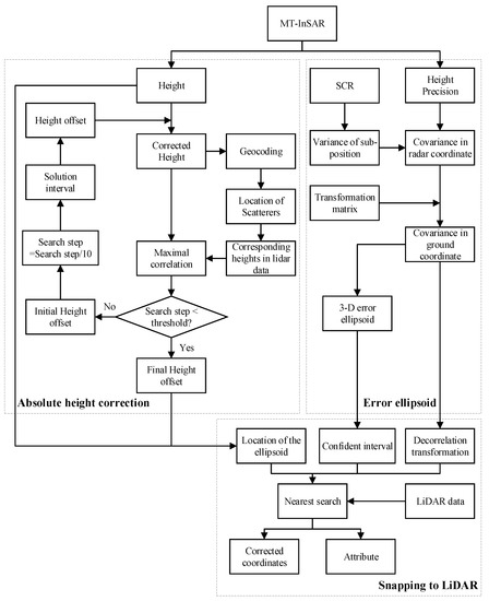
Figure 1.
Flowchart of the attribution of the InSAR observations using LiDAR data. There are three main steps: (1) absolute height correction; (2) error ellipsoid estimation; and (3) snapping to the LiDAR point cloud.
2.2.1. Absolute Height Correction
For a scatterer located at in terrestrial coordinates with a corresponding zero Doppler coordinate , we obtain the position state vector and velocity vector of the satellite using azimuth time t. The range time is indicated by r. The position is now determined by solving three equations, called Doppler–Range–Ellipsoid equations, which are defined as [1,6,37,38]
where a and b denote the semi-major and semi-minor axis of the reference ellipsoid, respectively. represents the distance from scatterer P to the satellite and H is the height relative to the reference ellipsoid.
Because the phase observations are wrapped, the absolute phase difference with respect to the ellipsoid cannot be determined, leading to a coordinate offset for all scatterers. Depending on the position of the scatterer in the image, which leads to a different local incidence angle, the estimated horizontal coordinate offset varies over the image. Since the estimated heights of all scatterers are related to a specified reference, we propose a solution search method to estimate the height offset with the help of grid data obtained by LiDAR point cloud. In each search, we add an initial height offset to the heights of all scatterers and update their coordinates. Then, the heights of corresponding LiDAR point cloud are extracted using the new coordinates of all radar scatterers. Furthermore, to evaluate the similarity between the heights of radar scatterers and that of point cloud, we calculate the Pearson correlation coefficient [39], which is defined as
where N is the number of radar scatterers, and and denote the standard deviation and the average, respectively. denotes the height of the radar scatterers while denotes that of the LiDAR point cloud. Pearson’s correlation coefficient is used to evaluate the similar tendency of two datasets, irrespective of the absolute value of the difference.
Setting an initial search interval and search step for the height offset, we repeat the calculation and obtain the corresponding correlations. In the end, the height offset candidate is located at maximal correlation. To improve the efficiency and obtain a result with high precision, the solution search approach is conducted several times with different search steps. For example, in the first search, we set a loose search interval and the search step is set to 1 m. In the following search, the initial height offset is used to determine a smaller search interval and the step is set to a smaller value as well. We repeat the process until the search step satisfies with the desired precision.
To estimate the height offset, it is not required to have LiDAR over the entire area covered by the radar, a small region may suffice, which also decreases the computational burden. Note that our matching method is expected to result in a height offset estimation that has a higher precision than that by single point correction, such as using GNSS or levelling.
2.2.2. Generating the Positioning Error Ellipsoid
The uncertainty in the position of the scatterers is determined by the covariance matrix, and the 3D error ellipsoid is the geometric representation of the covariance matrix. In radar coordinates, the position of a scatterer is described using the range, azimuth and cross-range coordinates [22], denoted as . The variance of the sub-position in azimuth and range is obtained using the estimated SCR [17]
where denotes the oversampling factor, which is set to 1 in our study. Based on the work of Adam et al. [40], the temporal is defined using the normalized amplitude dispersion index [3], described as
The variance of the position along the cross-range direction can be obtained by the height precision described in Section 2.1 and the radar geometry, which is described as . Hence, the VC matrix of the position in radar coordinate is defined as With the estimated absolute height offset, we obtain the corrected ground coordinates of all scatterers. After the geocoding step, we obtain scatterers in both the radar and ground coordinates and the datum transformation matrix is obtained by the S-transformation [33]. Furthermore, the VC matrix of the position of a scatterer in ground coordinates can be obtained using the propagation law of variances as
where the elements of the VC matrix are the variance and covariance in ground coordinates, denoted by . Based on this VC matrix, the error ellipsoid can be generated for each scatterer. The corrected coordinates of the scatterers estimated by the absolute heights are used as the center of the error ellipsoid. Setting a significance level , the size of the error ellipsoid, i.e. the three semi-axis lengths of the ellipsoid, are obtained by the eigenvalues of [17].
2.2.3. Snapping to the Point Cloud
The LiDAR point cloud is used to correct the locations of the radar scatterers and to add properties to them. It is worth noting that most coherent radar scatterers are related to man-made structures, such as buildings, bridges, and railways, while the LiDAR point cloud contains all kinds of geo-objects. However, some part of point clouds, e.g. vegetation and water, should be removed, since these objects cannot provide coherent scatterers.
A nearest neighbor search process with respect to the radar geometry estimation is used to snap the scatterers to their most likely point in the point cloud [20,21]. Considering the full covariance matrix of each radar scatterer, a Whitening transform is adopted to decorrelate the dimensions of the data coordinates. Given a data matrix with the VC matrix , two matrices and are obtained using the eigenvalue decomposition
where is eigenvector matrix and is a diagonal matrix whose diagonal elements are eigenvalues. Thus, we can transform the original data matrix into a new data matrix [41]
In the new coordinates, the unit of Euclidean distance is rather than meters, so the errors in different dimensions exhibit a normal distribution. Thus, the ellipsoids become spheres and the closest point, in Euclidian distance, is the most likely one. Additionally, a kd tree search algorithm [42] with a time complexity of is conducted to search the nearest neighbor. This algorithm is faster when the number of points is large.
After establishing the relationship between the point cloud and radar scatterers, the coordinates as well as the attributes of the point cloud are assigned to those of the radar scatterers.
2.3. Quality Metrics
During the estimation in the MT-InSAR process, we derive the precision of the parameters. Here, we summarize the quality metrics for assessing the performance using MT-InSAR considering both the deformation time series and the radar geometry.
2.3.1. Temporal Coherence
The temporal coherence estimator is an indicator for evaluating the deviation between the deformation time series and the estimated deformation model, which is defined as [6]
where m is the number of SAR images, is the phase component related to the displacement including modeled and un-modeled deformation and is the model phase. The coherence ranges between 0 and 1. Low coherence indicates large unmodeled deformation and/or large phase noise.
2.3.2. Dilution of Precision
Dilution of Precision (DoP) describes the geometric contribution to the quality of the parameters, which is defined using the covariance matrix of the Line of Sight (LOS) vector decomposition. Considering the application of railway monitoring, the displacement vector in a local, asset-fixed, right-handed Cartesian coordinate system, as defined in [43], is introduced. These coordinates describe the deformation in transversal, longitudinal, and normal directions, respectively. Longitudinal direction is along the rail track, while the transversal direction represents the cross-track direction. The normal direction is orthogonal to the transversal-longitudinal plane (see [43]).
A LOS vector decomposition can be conducted if at least three LOS observations with different viewing geometries are available, for the same object. If this condition cannot be met, optional constraints may be introduced, e.g. the assumption that deformation in a specific direction can be neglected. Under this constraint, we construct the covariance matrix with a different number of LOS observations.
- One track. If only one LOS observation is available, we may decide to evaluate only the projection of the deformation vector onto the normal direction, assuming that the longitudinal and transversal directions may be negligible. Here, we introduce pseudo-observations and , which are set to zero. Supposing that denote the transformation matrix from local coordinate to ground coordinate [43], the relationship between the displacement vector and LOS observation is defined as
- Two tracks. If two LOS observations are available, we may decide to assume that deformation in the longitudinal direction is negligible, by using a pseudo-observation to be equal to zero. Then, the relationship between the displacement vector and LOS observations is defined aswhere is the flight azimuth angle (heading) of the satellite.
- Three or more tracks. If at least three LOS observations are available, the LOS decomposition can be solved directly, as long as the viewing geometries are significantly different. The relationship between the displacement vector and LOS observations is defined as
The variance matrix of the displacement vector is obtained using the error propagation law
where denotes the design matrix and is the VC matrix of the LOS observations.
The DoP is obtained using covariance matrix of the displacement vector [43]
where is the determinant operator. A smaller DoP value indicates a higher quality of the parameters.
2.3.3. Sensitivity
Sensitivity is used to assess whether a deformation is observable with the LOS observations, which is defined as the modulus of the inner product [43]
where denotes the LOS unit vector from the scatterer to the satellite. This indicator ranges between 0 and 1. A sensitivity of 1 shows the geometric quality of the LOS deformation is optimal while a sensitivity of 0 means the deformation cannot be detected using the LOS measurements.
3. Results and Discussion
Subsequently, we discuss the used data sources for the area of interest, the estimation results, coordinate corrections and point classification, and the analysis of the results.
3.1. Data Resources
The amplitude-augmented interferometric processing is demonstrated using 48 RadarSAT-2 XF images acquired between March 2015 and August 2018 over Zaltbommel, The Netherlands. The selected dataset covers 10 km of railway and a buffer zone of 2 km width. The slant-range and azimuth pixel spacings are 2.66 m and 2.47 m, respectively. An external digital elevation models (DEM) is not needed due to the lack of significant topography. However, the residual topographic phase of each coherent scatterer is estimated in the time series analysis. The temporal baseline range is 870 days, while the spatial baseline range is 280 m. Temperatures are recorded per hour and interpolated to the time of the SAR acquisition [44].
The used airborne LiDAR product, Actueel Hoogtebestand Nederland 3 (AHN3), covering the entire territory of the Netherlands [45], contains both a DEM and a Digital Surface Model (DSM) with a point density of 12.7 pts/m and a grid of 0.5 m × 0.5 m with an elevation accuracy of less than 5 cm systematic and 5 cm stochastic. Given this point spacing, an object of 2 m × 2 m has an error of maximum 25 cm, which is less than one quarter of a pixel in the image resolution of RadarSAT-2 XF. Furthermore, five classes (i.e., ground, building, water, civil structure, and unclassified) are included in the the newest version of AHN3 data, which were updated in 2019. In this case, the AHN3 point cloud covers the selected railway within a buffer zone of 500 m width. All software used for InSAR time series analysis and classification was coded in MATLAB.
3.2. Radar Observations along the Railway
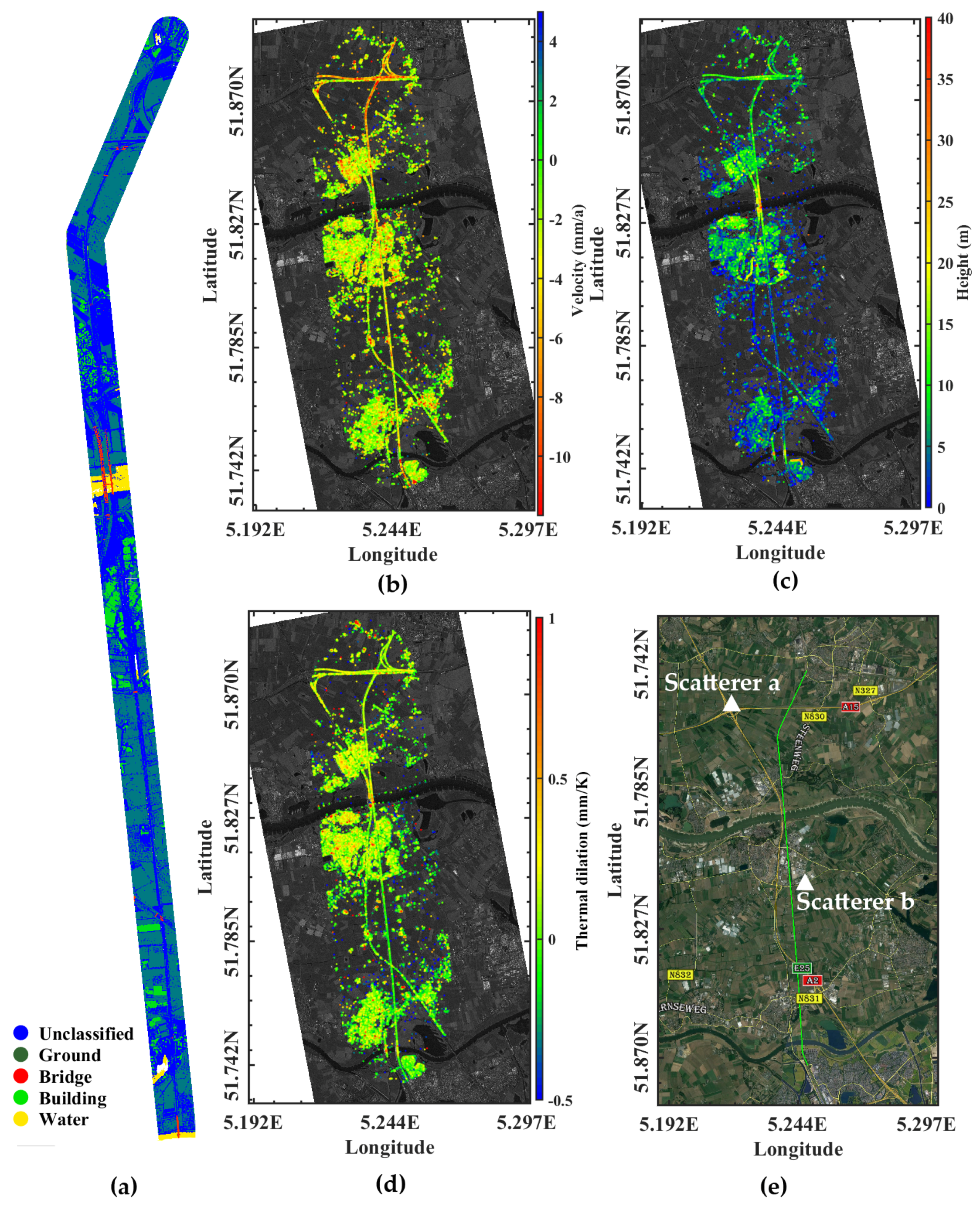
Figure 2a shows the AHN3 point cloud along the railway with classification and Figure 2e denotes the location of the railway. Both CCS and TCS are processed and the final result maps contain about CCS and TCS (see Figure 2b–d). Since the number of CCS is much larger than the number of TCS, apparently most areas did not change during the acquired time. The deformation velocities range from to mm/a, and the scatterers along the railway are homogeneously distributed. The velocity map shows that the settlement along the north of the railway is larger than that along the south. The heights range from 0 to m and the thermal dilation range from to mm/K. Since thermal dilation depends on the material of the radar scatterer, it only shows a limited variation over the area. With the help of the TCS, we significantly improve the point density and extract more information using the radar observations.
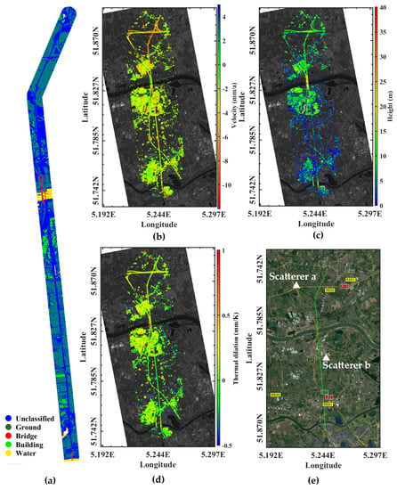
Figure 2.
(a) AHN3 point cloud along the railway and its buffer zone with classifications. Estimated parameters on both CCS and TCS: (b) velocity map; (c) height map; (d) thermal dilation; and map. (e) Location of the railway (green line).
The precision of the estimated parameters is obtained, and the histograms of the estimated height and deformation velocities are shown in Figure 3. The precision of the estimated height is used to generate the error ellipsoid (cf. Section 2.2.2) while that of velocity is used to calculate the DoP (cf. Section 2.3.2).
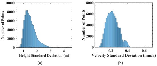
Figure 3.
Histograms of the precision: (a) height; and (b) deformation velocity.
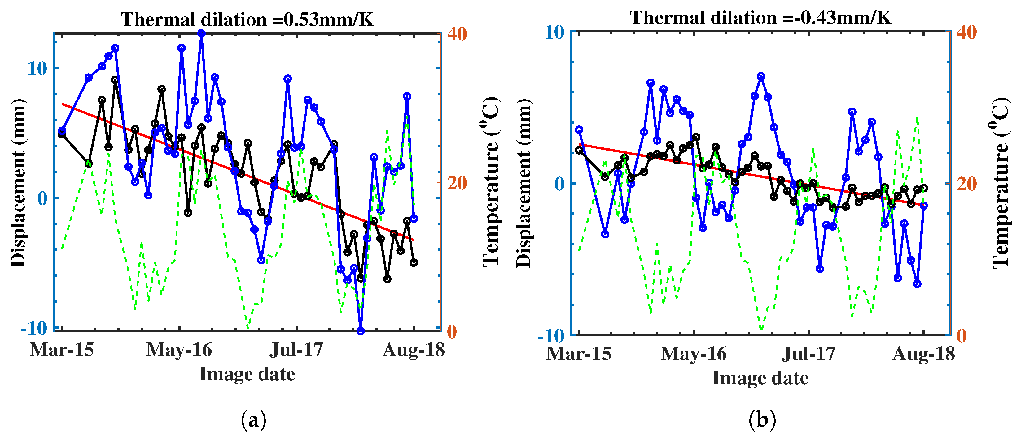
Figure 2c shows that some scatterers are strongly related to the temperature with a maximum thermal dilation of more than 0.5 mm/K. Two scatterers are selected and their displacement time series are shown in Figure 4. After removing the thermal dilation phase, the displacement time series becomes smoother with decreasing RMS and it is easier to detect phase anomalies.
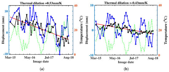
Figure 4.
Displacement time series of two selected scatterers with strong thermal dilation: (a) the RMS of the displacement drops from 4.2 to 1.0 mm; and (b) the RMS of the displacement drops from 5.2 to 2.3 mm. Green dot line, temperature per acquisition; red line, linear deformation time series; blue line, deformation time series without temperature correction including linear deformation, nonlinear deformation, temperature motion and noise; black line, temperature-corrected deformation time series including linear deformation, nonlinear deformation and noise.
3.3. Coordinate Correction and Classification
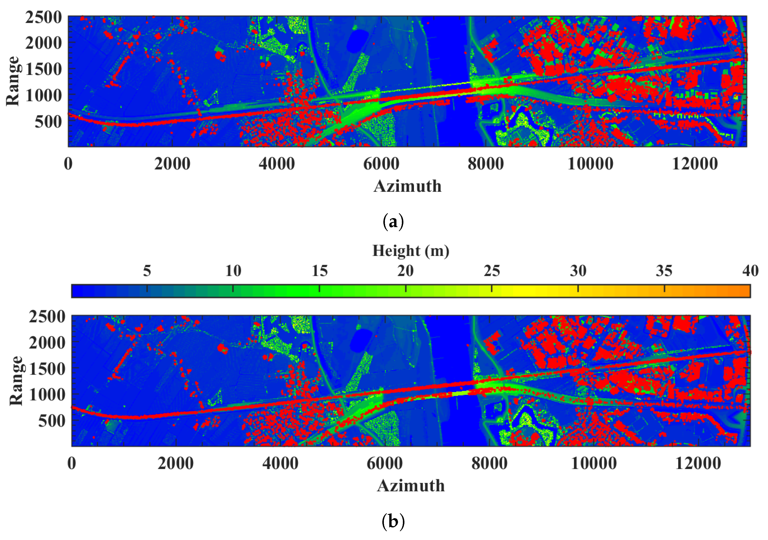
During the absolute height correction with the LiDAR data, the iterative search process is repeated three times, leading to a height offset estimate with centimeter precision. This height offset results in an additional horizontal offset, as shown by comparing the radar scatterers (red points) with the Lidar point cloud (see Figure 5a). After the height correction (cf. Figure 5b), the radar scatterers align with the Lidar points indicating infrastructure.
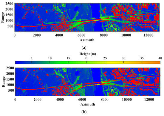
Figure 5.
Distribution of the radar scatterers (red dots) relative to the LiDAR data (height-colored dots): (a) coordinates of radar scatterers before height offset correction; and (b) coordinates of radar scatterers after height offset correction.
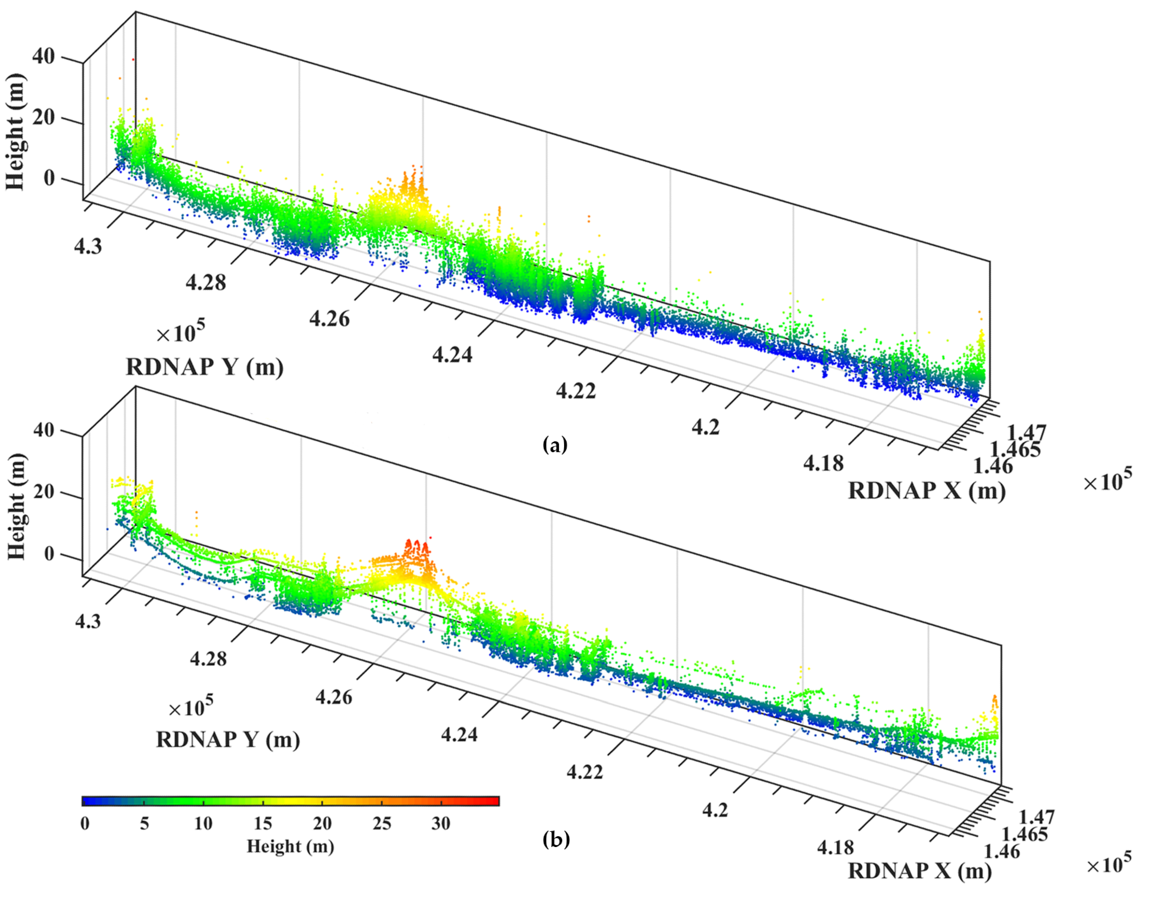
Setting the significance level to 0.005, we generated the error ellipsoids for all scatterers. The semi-axis length of the ellipsoid in the cross-range direction is much larger than the lengths of those of range and azimuth in radar coordinates. Subsequently, we applied a coordinate decorrelation and snapped the radar scatterers to the point cloud [20]. This process was conducted per point. Thus, a parallel processing approach can be adopted to improve the search efficiency. During the process, we discarded the scatterers that are not associated with any point in the cloud. Finally, we snapped 94% of the radar scatterers to a new position. The 3D height map of all radar scatterers with corrected coordinates is shown in Figure 6b. Figure 6a shows the same scatterers with the initial coordinates. Here, we project the geodetic coordinate [46] using RDNAPTRANS into the Dutch National Triangulation system RD and vertical NAP, denoted as RDNAP, which is referred to as ground coordinates in the following. In Figure 6a,b, it is more convenient to associate the radar scatterers with ground objects.
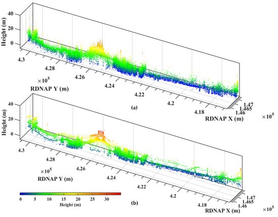
Figure 6.
3D map of radar scatterers (a) without and (b) with coordinate correction by LiDAR, showing a better separability of high and low objects.
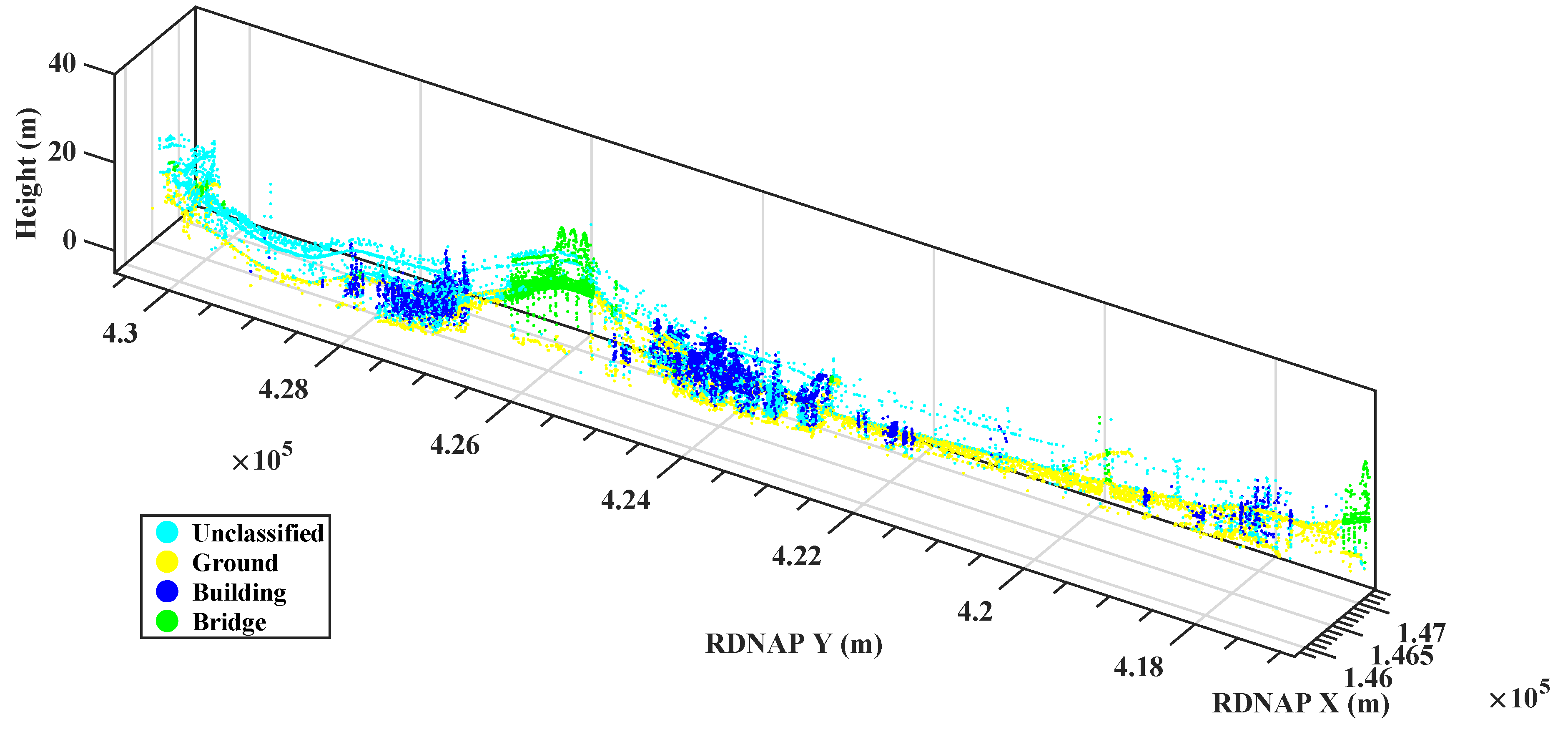
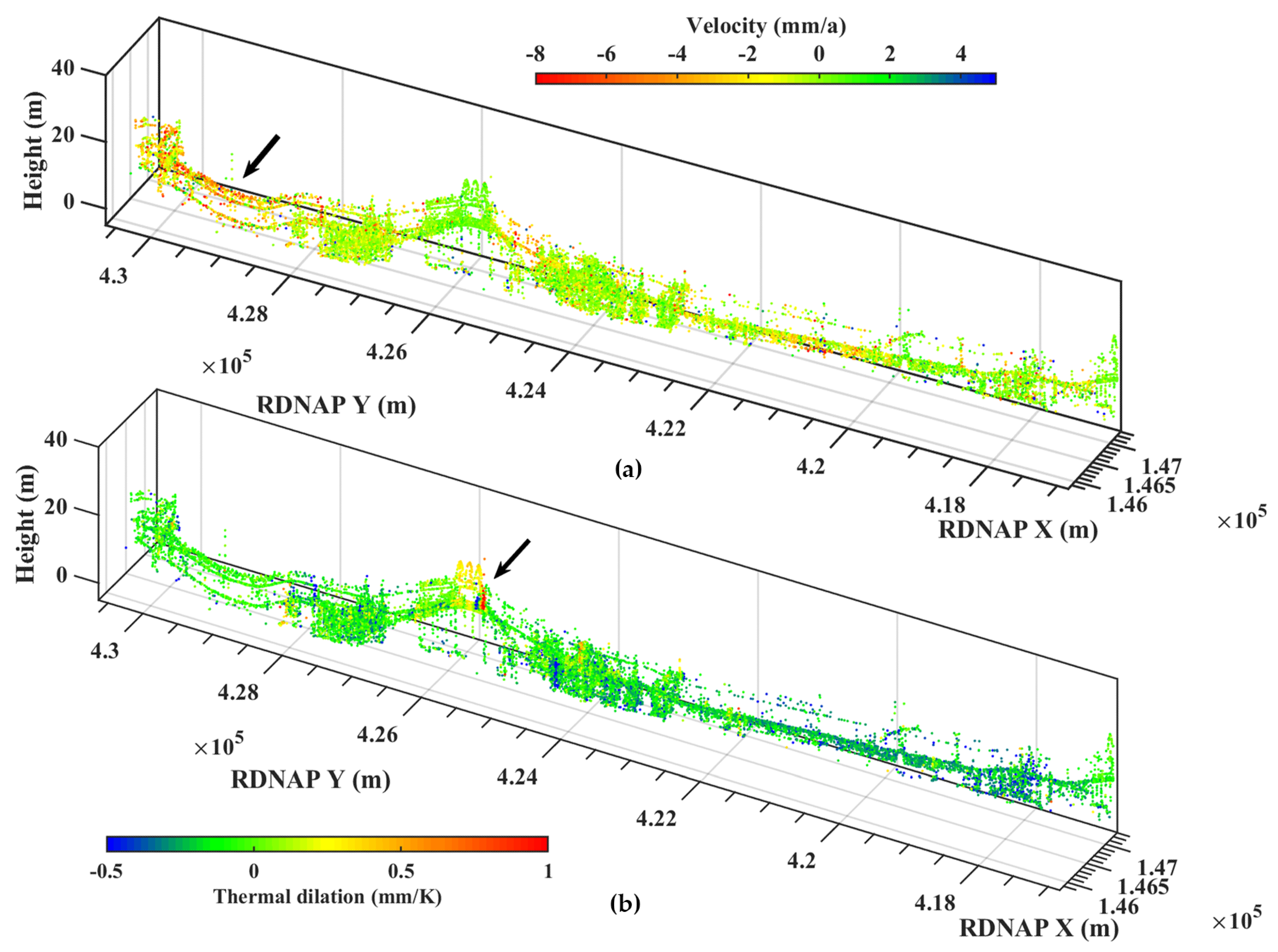
The classification of the LiDAR point cloud is transferred to the corresponding radar scatterers (see Figure 7). There are four classes in our result, i.e. bridge, ground, building, and unclassified, e.g., the catenary poles along the railway. Figure 8 shows the parameters of the scatterers with corrected coordinates. The scatterers on the bridge are very stable while those on the ground exhibit higher settlements (north area indicated by the black arrow) (see Figure 7 and Figure 8a). The thermal dilations on the bridge are larger than those of scatterers on the ground, which supports our classification (see Figure 8b).

Figure 7.
Classification of the radar scatterers with corrected coordinates based on their attribute to the LiDAR points, which are already classified.

Figure 8.
Parameters of the scatterers with corrected coordinates: (a) deformation velocity, demonstrating the instability of the north area; and (b) thermal dilation, showing the strong thermal dilation of the bridge structure.
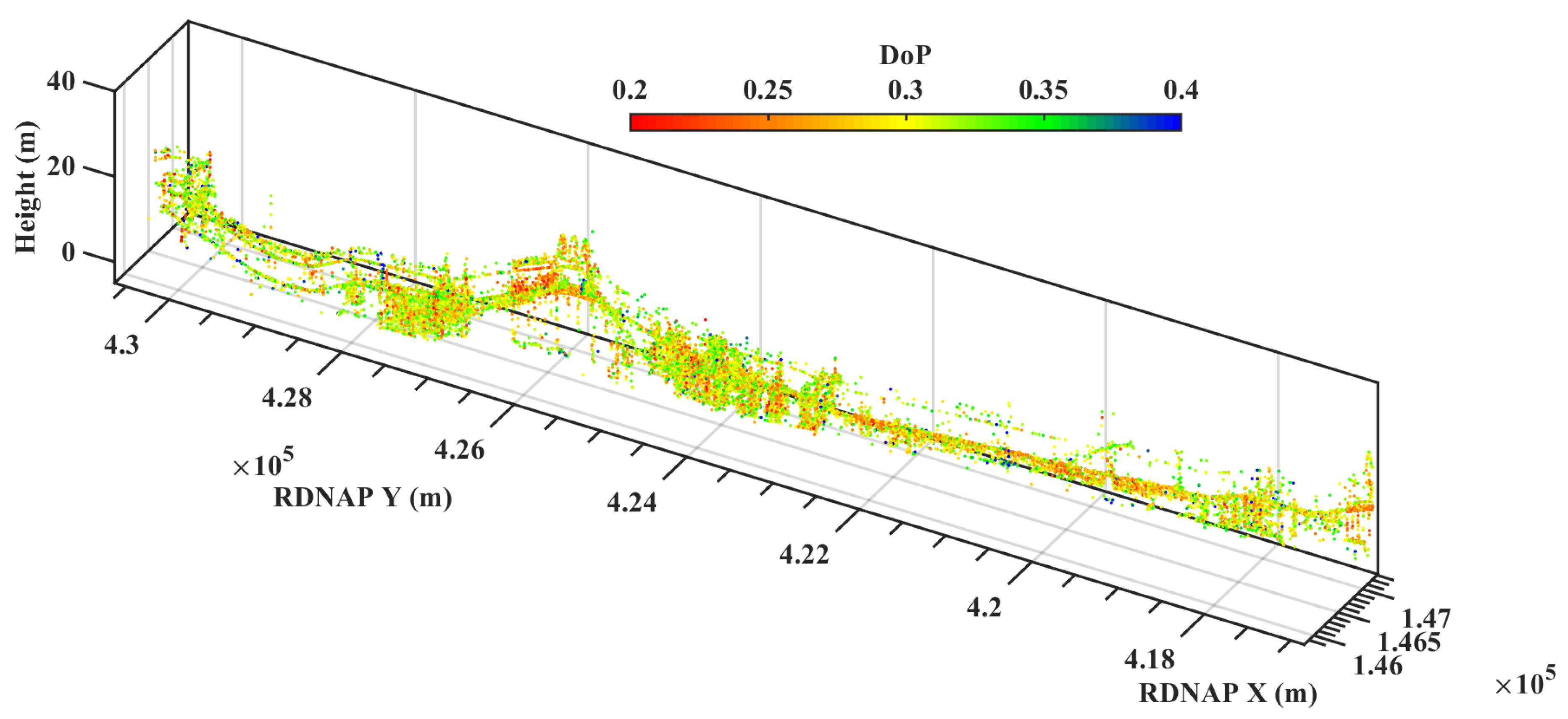
The quality metrics described in Section 2.3 are calculated for all scatterers. For 96% of the scatterers, the ensemble coherences are larger than 0.75, which implies that the deformation time series derived from the MT-InSAR process has a high precision, and that the model fits generally well.Considering the DoP and sensitivity, we use Equation (16) of one LOS observation for the calculation. Figure 9 shows the DoP values of all scatterers, ranging between 0.1 and 0.5, where a larger DoP value indicates a lower quality. Most scatterers have a DoP of approximately 0.25. Since the orientation of the selected railway section is north–south, the sensitivity of all scatterers is comparable. The sensitivities of most scatterers are around 0.57, indicating a reasonable capability of deformation detection (see Section 2.3.3).
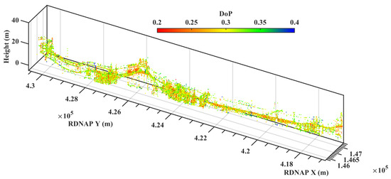
Figure 9.
DoP values of radar scatterers with correct coordinates, showing the qualities of different scatterers.
3.4. Comparison and Analysis
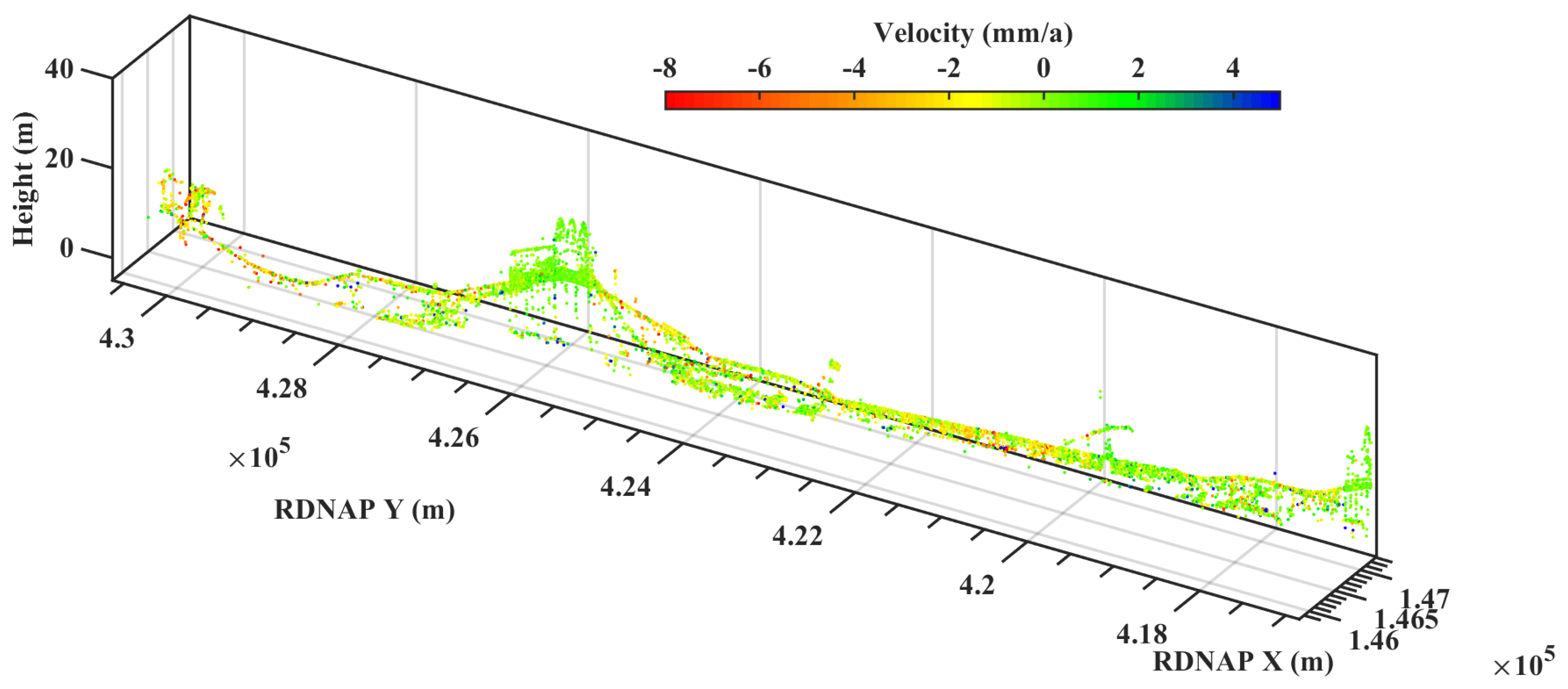
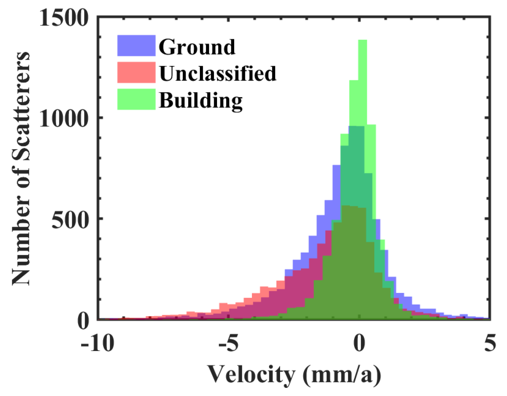
Based on the classification (see Figure 8a), scatterers within a specified class can be extracted for further analysis. For example, if we are only interested in the deformation of the ground and the bridge, scatterers with other classifications can be removed. The deformation velocity of the selected scatterers is shown in Figure 10. Compared to Figure 8a, this shows that the classification leads to a successful isolation of the scatterers representative of the railway track. Additionally, Figure 11 shows the histograms of the deformation velocity within different classes. Scatterers from different classes exhibit a different distribution. For example, scatterers on buildings are relatively stable with deformation velocities ranging from mm/a to mm/a, while other scatterers (on the ground or on catenary poles) show more variable deformation rates with maximum rates exceeding 10 mm/a. Thus, the classification improves the interpretation relative to the original mixed deformation signal.
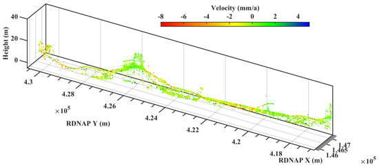
Figure 10.
Deformation velocity of the scatterers with selected classifications (bridge and ground), indicating the deformation related to the railway.
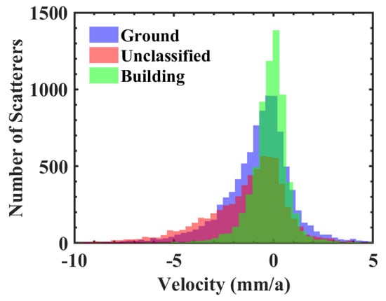
Figure 11.
Histograms of the deformation velocity within different classes, showing a better interpretation of deformation signals with classified scatterers.
Three segments of the railway are selected to show more detail. We compare the height map of radar scatterers with that of the LiDAR point cloud (see Figure 12). In Figure 12a,b, the density of radar scatterers is high enough to show the structure of the railway. Comparing Figure 12d,f, the density of the scatterers along the second and third segment is different. The second segment of the railway is east–west with a scatterer density of 0.51 pt/m while the third is north–south with a scatterer density of 0.72 pt/m, which means that the density of coherent scatterers depends on the orientation of the railway, relative to the satellite heading.
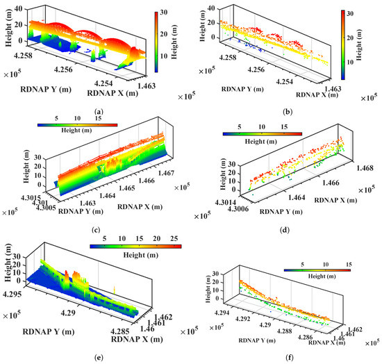
Figure 12.
(a–f) Comparison of the height model between LiDAR data and radar scatterers. The first column corresponds to the LiDAR data and the second column corresponds to the radar scatterers. Each row corresponds to a selected segment of the railway.
Figure 13 shows the deformation velocity and thermal dilation of scatterers from bridge and ground. The deformation velocity of scatterers on the bridge is smaller than that of scatterers on the ground, while the thermal dilation of the scatterers on the bridge is larger than that of scatterers on the ground. In addition, the thermal dilation of the scatterers on the bridge arches are also greater than that of scatterers on the bridge deck. Thus, all results support the classification results.

Figure 13.
Parameters of the selected bridge: (a) velocity map, showing the transitions of velocity between bridge and ground; and (b) thermal dilation map, showing the strong thermal dilation on the bridge structure.
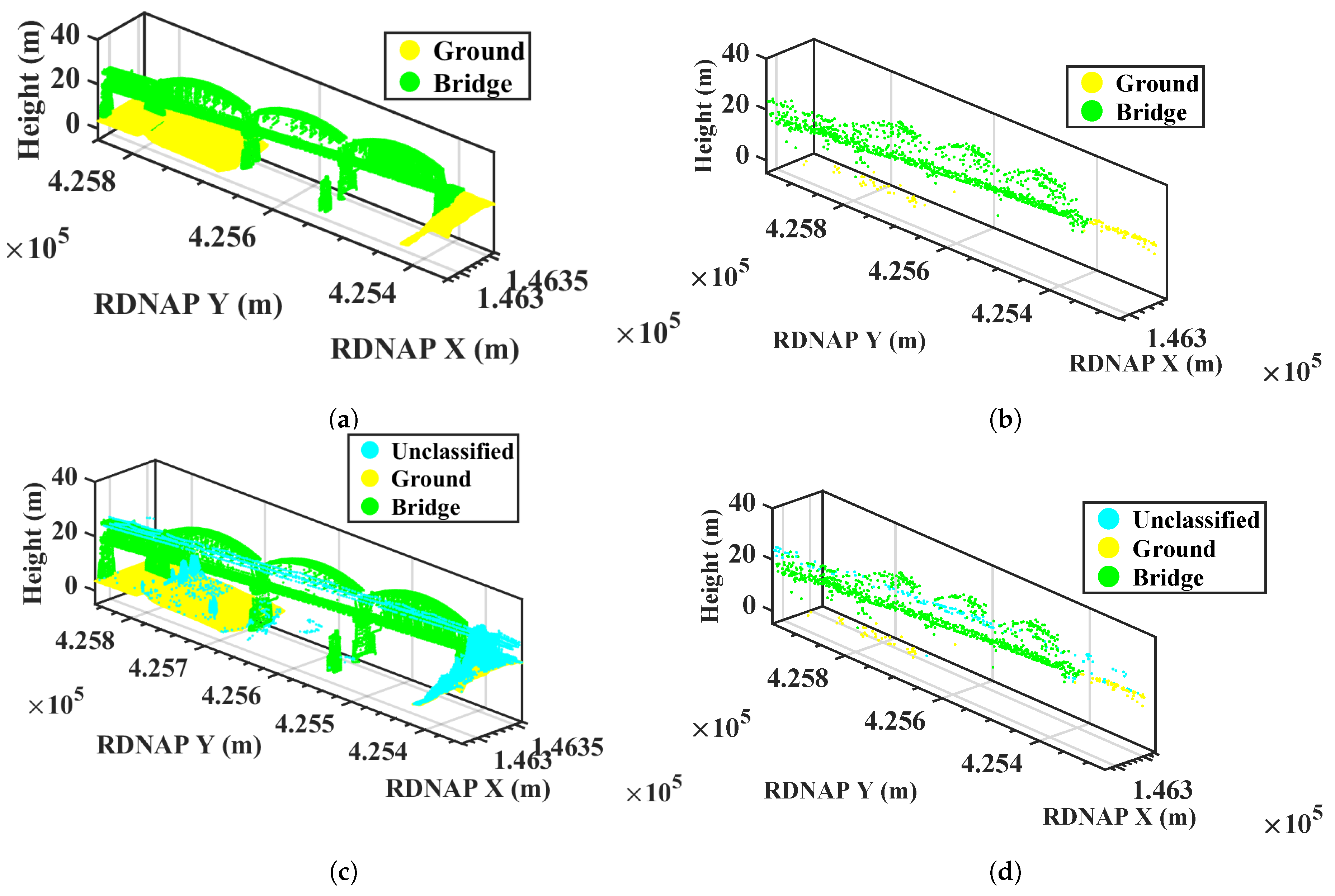
In the LiDAR point clouds, there is a class of “unclassified” points including trees, power lines and other geo-objects. Some objects, such as catenary poles, are coherent scatterers while others (vegetation) can never be coherent scatterers because of the leaf cover, at least part of the year. Therefore, we evaluate whether this class should be used in our classification (see Figure 14). In Figure 14a,c, some scatterers in the unclassified group are related to the poles, which are important to evaluate the state of the railway. In Figure 14b,d, some scatterers related to the power lines are misclassified as scatterers on the ground and a few scatterers are missing if we neglect the unclassified group. Figure 15 shows the classification maps of the other two segments. We also found many scatterers related to the catenary poles along the railway. Therefore, it is necessary to include the “unclassified” group during the classification.
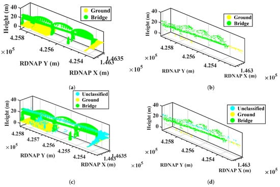
Figure 14.
Comparison of classification map: (a,c) classification maps of LiDAR; (b,d) classification maps of radar scatterers; (a,b) classification maps without unclassified one; and (c,d) classification maps with unclassified one.
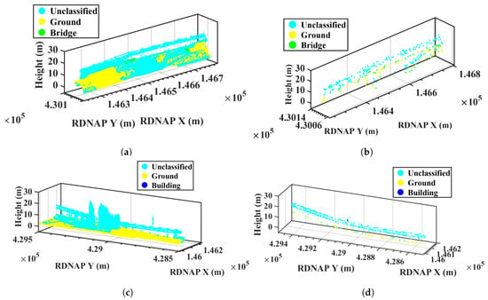
Figure 15.
Classification maps of two selected areas: (a,c) classification maps of LiDAR; and (b,d) classification maps of radar scatterers, showing the importance of including the unclassified group.
4. Conclusions
While MT-InSAR is a useful tool for structural health monitoring of large structures, there are limitations in the interpretation of the data due to the imperfect attribution of radar scatterers to physical objects. This is mainly due to the relative nature of the elevation estimates and the limited positioning accuracy. With the help of LiDAR data, we can overcome these limitations and increase the value of the MT-InSAR results. A structural health monitoring approach for railway systems is proposed and demonstrated combining MT-InSAR and LiDAR point clouds. A case study using RadarSAT-2 XF data over the Netherlands was conducted. A novel amplitude-augmented interferometric processing approach, including temperature coefficients, demonstrates a good point density of radar observations. Quality metrics such as the ensemble coherence, the DoP value, the sensitivity and the covariance matrix of all radar scatterers are calculated given the radar and infrastructure geometry. This way railway asset managers can select and interpret observations based on different combinations of the quality metrics. Results of snapping radar scatterers to the corresponding laser points using the 3D confidence ellipsoid show that LiDAR can not only be used to improve the positioning of the scatterers but to classify the scatterers as well. The classification enables the isolation of specific types of radar scatterers, leading to an improved interpretation of the deformation signal. With the help of the classification, it is easier to interpret the deformation signals, in particular over transition zones. If more datasets are available, an increasing number of attributes can yield more details in the classification.
Author Contributions
F.H., F.J.v.L., L.C., J.W. and R.F.H. conceived and designed the experiments; F.H. processed the InSAR data and LiDAR point cloud; and F.H. and F.J.v.L. wrote the main manuscript.
Funding
This research was funded in part by the China Scholarship Council (201706260149), the State Key Development Program for Basic Research of China (No.2013CB733304) and the National Nature Science Foundation of China (No.41674003).
Conflicts of Interest
The authors declare no conflict of interest.
References
- Hanssen, R.F. Radar Interferometry: Data Interpretation and Error Analysis; Kluwer Academic Publishers: Dordrecht, The Netherlands, 2001. [Google Scholar] [CrossRef]
- Ferretti, A.; Prati, C.; Rocca, F. Permanent Scatterers in SAR Interferometry. In Proceedings of the International Geoscience and Remote Sensing Symposium, Hamburg, Germany, 28 June–2 July 1999; pp. 1–3. [Google Scholar]
- Ferretti, A.; Prati, C.; Rocca, F. Permanent Scatterers in SAR Interferometry. IEEE Trans. Geosci. Remote Sens. 2001, 39, 8–20. [Google Scholar] [CrossRef]
- Kampes, B.M.; Hanssen, R.F. Ambiguity Resolution for Permanent Scatterer Interferometry. IEEE Trans. Geosci. Remote Sens. 2004, 42, 2446–2453. [Google Scholar] [CrossRef]
- Hooper, A.; Zebker, H.; Segall, P.; Kampes, B. A new method for measuring deformation on volcanoes and other non-urban areas using InSAR persistent scatterers. Geophys. Res. Lett. 2004, 31, L23611. [Google Scholar] [CrossRef]
- Van Leijen, F.J. Persistent Scatterer Interferometry Based on Geodetic Estimation Theory; NCG: Amersfoort, The Netherlands, 2014. [Google Scholar]
- Özer, I.E.; Rikkert, S.J.; van Leijen, F.J.; Jonkman, S.N.; Hanssen, R.F. sub-seasonal Levee Deformation observed Using satellite Radar Interferometry to enhance Flood protection. Sci. Rep. 2019, 9, 2646. [Google Scholar] [CrossRef] [PubMed]
- Özer, I.E.; van Leijen, F.J.; Jonkman, S.N.; Hanssen, R.F. Applicability of satellite radar imaging to monitor the conditions of levees. J. Flood Risk Manag. 2018, 12509, 1–16. [Google Scholar] [CrossRef]
- Perissin, D.; Wang, T. Time-series InSAR applications over urban areas in China. IEEE J. Sel. Top. Appl. Earth Obs. Remote Sens. 2011, 4, 92–100. [Google Scholar] [CrossRef]
- Costantini, M.; Falco, S.; Malvarosa, F.; Minati, F.; Trillo, F.; Vecchioli, F. Persistent scatterer pair interferometry: Approach and application to COSMO-SkyMed SAR data. IEEE J. Sel. Top. Appl. Earth Obs. Remote Sens. 2014, 7, 2869–2879. [Google Scholar] [CrossRef]
- Wu, J.; Hu, F. Monitoring ground subsidence along the Shanghai Maglev zone using TerraSAR-X images. IEEE Geosci. Remote Sens. Lett. 2017, 14, 117–121. [Google Scholar] [CrossRef]
- Chang, L.; Dollevoet, R.P.; Hanssen, R.F. Nationwide railway monitoring using satellite SAR interferometry. IEEE J. Sel. Top. Appl. Earth Obs. Remote Sens. 2017, 10, 596–604. [Google Scholar] [CrossRef]
- Wang, H.; Chang, L.; Markine, V. Structural health monitoring of railway transition zones using satellite radar data. Sensors 2018, 18, 413. [Google Scholar] [CrossRef]
- Ribeiro, D.; Calçada, R.; Ferreira, J.; Martins, T. Non-contact measurement of the dynamic displacement of railway bridges using an advanced video-based system. Eng. Struct. 2014, 75, 164–180. [Google Scholar] [CrossRef]
- Bowness, D.; Lock, A.; Powrie, W.; Priest, J.; Richards, D. Monitoring the dynamic displacements of railway track. Proc. Inst. Mech. Eng. Part F J. Rail Rapid Transit 2007, 221, 13–22. [Google Scholar] [CrossRef]
- Iryani, L.; Setiawan, H.; Dirgantara, T.; Putra, I.S. Development of a railway track displacement monitoring by using digital image correlation technique. Appl. Mech. Mater. 2014, 548, 683–687. [Google Scholar] [CrossRef]
- Dheenathayalan, P.; Small, D.; Schubert, A.; Hanssen, R.F. High-precision positioning of radar scatterers. J. Geod. 2016, 90, 403–422. [Google Scholar] [CrossRef]
- Yang, M.; Dheenathayalan, P.; Chang, L.; Wang, J.; Lindenbergh, R.C.; Liao, M.; Hanssen, R.F. High-precision 3D geolocation of persistent scatterers with one single-Epoch GCP and LIDAR DSM data. In Proceedings of the ESA Living Planet Symposium 2016, Prague, Czech Republic, 9–13 May 2016. [Google Scholar]
- Mahapatra, P.; van der Marel, H.; van Leijen, F.; Samiei-Esfahany, S.; Klees, R.; Hanssen, R. InSAR datum connection using GNSS-augmented radar transponders. J. Geod. 2018, 92, 21–32. [Google Scholar] [CrossRef]
- Van Natijne, A. Locating PS-InSAR Derived Deformation Using LiDAR Point Clouds. Master’s Thesis, Delft University of Technology, Delft, The Netherlands, 2018. [Google Scholar]
- Van Natijne, A.; Lindenbergh, R.C.; Hanssen, R.F. Massive linking of PS-InSAR deformations to a national airborne laser point cloud. Int. Arch. Photogramm. Remote Sens. Spat. Inf. Sci. 2018, 42, 2. [Google Scholar] [CrossRef]
- Dheenathayalan, P.; Small, D.; Hanssen, R.F. 3-D Positioning and Target Association for Medium-Resolution SAR Sensors. IEEE Trans. Geosci. Remote Sens. 2018, 56, 6841–6853. [Google Scholar] [CrossRef]
- Dheenathayalan, P.; Cuenca, M.C.; Hoogeboom, P.; Hanssen, R.F. Small reflectors for ground motion monitoring with InSAR. IEEE Trans. Geosci. Remote Sens. 2017, 55, 6703–6712. [Google Scholar] [CrossRef]
- Ferretti, A.; Colesanti, C.; Perissin, D.; Prati, C.; Rocca, F. Evaluating the effect of the observation time on the distribution of SAR Permanent Scatterers. In Proceedings of the Third International Workshop on ERS SAR Interferometry, ‘FRINGE03’, Frascati, Italy, 1–5 December 2003; pp. 1–5. [Google Scholar]
- Perissin, D.; Ferretti, A. Urban-Target Recognition by Means of Repeated Spaceborne SAR Images. IEEE Trans. Geosci. Remote Sens. 2007, 45, 4043–4058. [Google Scholar] [CrossRef]
- Zhang, L. Temporarily Coherent Point SAR Interferometry. Ph.D. Thesis, The Hong Kong Polytechnic University, Hong Kong, China, 2012. [Google Scholar]
- Hu, F.; Wu, J.; Chang, L.; Hanssen, R.F. Incorporating Temporary Coherent Scatterers in Multi-Temporal InSAR Using Adaptive Temporal Subsets. IEEE Trans. Geosc. Remote Sens. 2019, 57, 7658–7670. [Google Scholar] [CrossRef]
- Crosetto, M.; Monserrat, O.; Cuevas-González, M.; Devanthéry, N.; Luzi, G.; Crippa, B. Measuring thermal expansion using X-band persistent scatterer interferometry. ISPRS J. Photogramm. Remote Sens. 2015, 100, 84–91. [Google Scholar] [CrossRef]
- Chang, L.; Hanssen, R.F. A probabilistic approach for InSAR time-series postprocessing. IEEE Trans. Geosci. Remote Sens. 2016, 54, 421–430. [Google Scholar] [CrossRef]
- Monserrat, O.; Crosetto, M.; Cuevas, M.; Crippa, B. The thermal expansion component of persistent scatterer interferometry observations. IEEE Geosci. Remote Sens. Lett. 2011, 8, 864–868. [Google Scholar] [CrossRef]
- Verhagen, S.; Teunissen, P.J. New global navigation satellite system ambiguity resolution method compared to existing approaches. J. Guid. Control Dyn. 2006, 29, 981–991. [Google Scholar] [CrossRef]
- Ferretti, A.; Prati, C.; Rocca, F. Nonlinear Subsidence Rate Estimation using Permanent Scatterers in Differential SAR Interferometry. IEEE Trans. Geosci. Remote Sens. 2000, 38, 2202–2212. [Google Scholar] [CrossRef]
- Baarda, W. S-Transformations and Criterion Matrices, 2nd ed.; Publications on Geodesy, New Series; Netherlands Geodetic Commission: Delft, The Netherlands, 1981; Volume 5, p. 168. [Google Scholar]
- Kampes, B.M. Radar Interferometry; Springer: Houten, The Netherlands, 2006. [Google Scholar]
- Ataei, A. Improved Qrginv algorithm for computing Moore-Penrose inverse matrices. ISRN Appl. Math. 2014, 2014, 1–5. [Google Scholar] [CrossRef]
- Johnson, R.A.; Wichern, D.W. Applied Multivariate Statistical Analysis; Prentice Hall: Upper Saddle River, NJ, USA, 2002; Volume 5. [Google Scholar]
- Montazeri, S.; Rodríguez González, F.; Zhu, X. Geocoding Error Correction for InSAR Point Clouds. Remote Sens. 2018, 10, 1523. [Google Scholar] [CrossRef]
- Schreier, G. SAR Geocoding: Data and Systems; Wichmann Verlag: Karlsruhe, Germany, 1993. [Google Scholar]
- Ahlgren, P.; Jarneving, B.; Rousseau, R. Requirements for a cocitation similarity measure, with special reference to Pearson’s correlation coefficient. J. Am. Soc. Inf. Sci. Technol. 2003, 54, 550–560. [Google Scholar] [CrossRef]
- Adam, N.; Kampes, B.M.; Eineder, M. Development of a scientific Persistent Scatterer System: Modifications for mixed ERS/ENVISAT time series. In Proceedings of the ENVISAT & ERS Symposium, Salzburg, Austria, 6–10 September 2004; p. 9. [Google Scholar]
- Stansbury, D. The Statistical Whitening Transform. Available online: https://theclevermachine.wordpress.com/tag/eigenvalue decomposition (accessed on 30 March 2019).
- Finkel, R.; Friedman, J.; Bentley, J. An algorithm for finding best matches in logarithmic expected time. ACM Trans. Math. Softw. 1977, 3, 209–226. [Google Scholar]
- Chang, L.; Dollevoet, R.P.; Hanssen, R.F. Monitoring line-infrastructure with multisensor SAR interferometry: Products and performance assessment metrics. IEEE J. Sel. Top. Appl. Earth Obs. Remote Sens. 2018, 11, 1593–1605. [Google Scholar] [CrossRef]
- KNMI. Available online: http://projects.knmi.nl/klimatologie/uurgegevens (accessed on 30 October 2018).
- Kadaster; Geonovum. Publieke Dienstverlening Op de Kaart (PDOK). Available online: https://www.pdok.nl/ (accessed on 30 November 2018).
- De Bruijne, A.; van Buren, J.; Kösters, A.; van der Marel, H. Geodetic Reference Frames in The Netherlands. Definition and Specification of ETRS89, RD and NAP, and Their Mutual Relationships; Netherlands Geodetic Commission: Delft, The Netherlands, 2005. [Google Scholar]
© 2019 by the authors. Licensee MDPI, Basel, Switzerland. This article is an open access article distributed under the terms and conditions of the Creative Commons Attribution (CC BY) license (http://creativecommons.org/licenses/by/4.0/).


