Article

Sea Surface Temperature in Global Analyses: Gains from the Copernicus Imaging Microwave Radiometer

1
Department of Meteorology, University of Reading, PO Box 243, Reading, RG6 6BB, UK
2
Department of Geography, Swansea University, Singleton Park, Swansea, SA2 8PP, UK
3
Met Office, FitzRoy Road, Exeter, EX1 3PB, UK
4
LERMA, Observatoire de Paris, 61 Av. de l’Observatoire, 75014 Paris, France
5
European Space Agency, European Space & Technology Centre, Keplerlaan 1, Postbus 299, 2200 AG Noordwijk, The Netherlands
*
Author to whom correspondence should be addressed.
Remote Sens. 2019, 11(20), 2362; https://doi.org/10.3390/rs11202362
Submission received: 9 August 2019 / Revised: 18 September 2019 / Accepted: 23 September 2019 / Published: 11 October 2019
(This article belongs to the Section Ocean Remote Sensing)

Abstract

:
Sea surface temperatures (SSTs) derived from passive microwave (PMW) observations benefit global ocean and SST analyses because of their near-all-weather availability. Present PMW SSTs have a real aperture-limited spatial resolution in excess of 50 km, limiting the spatial fidelity with which SST features, reflecting ocean dynamics, can be captured. This contrasts with the target resolution of global analyses of 5 to 10 km. The Copernicus Imaging Microwave Radiometer (CIMR) is a mission concept under consideration as a high-priority candidate mission for the expansion of the Copernicus space programme. This instrument would be capable of real aperture resolution < 15 km with low total uncertainties in the range 0.4–0.8 K for channels between 1.4 and 36.5 GHz, and a dual-view arrangement that further reduces noise. This paper provides a comparative study of SST uncertainty and feature resolution with and without the availability of CIMR in the future SST-observing satellite constellation based on a detailed simulation of CIMR plus infrared observations and the processing of global SST analyses with 0.05° final grid resolution. Simulations of CIMR data including structured errors were added to an observing system consisting of the Sea and Land Surface Temperature Radiometer (SLSTR) on Sentinel-3A and the Advanced Very High Resolution Radiometer (AVHRR) on MetOp-A. This resulted in a large improvement in the global root-mean-square error (RMSE) for SST from 0.37 K to 0.21 K for January and 0.40 K to 0.25 K for July. There was a particularly noticeable improvement in the performance of the analysis, as measured by the reduction in RMSE, for dynamical and persistently cloudy areas. Of these, the Aghulas Current showed an improvement of 43% in January and 48% in July, the Gulf Stream showed 70% and 44% improvements, the Southern Ocean showed 57% and 74% improvements, and the Maritime Continent showed 50% and 40% improvements, respectively.

Graphical Abstract

1. Introduction

Measurement of sea surface temperatures (SSTs) is crucial to the understanding and prediction of the atmosphere and ocean. The SST regulates the exchange of moisture and heat [1,2] between the two and thus controls the thermal structure of the upper ocean and sets the boundary conditions needed for numerical weather prediction (NWP). Errors in SST can lead directly to a decrease in NWP skill [3]. SSTs retrieved from infrared (IR) sensor data generally have superior spatial resolution (≈1 km) and retrieval accuracy (0.2 to 0.4 K) to passive microwave (PMW) sensors (≈50 km and 0.35 to 0.5 K, respectively, for recent and current missions) [4,5,6,7]. However, they are limited to cloud-free regions, whereas PMW sensors are able to make measurements through clouds. This greatly increases their coverage and makes them particularly important for regions of persistent cloud such as the high-latitudes in winter.
The Copernicus Imaging Microwave Radiometer (CIMR) is a mission concept under consideration as a high-priority candidate mission for the expansion of the Copernicus space programme (the Sentinels). The concept includes the deployment of a ≈7 m mesh antenna capable of real aperture resolution < 15 km at 6.9 GHz (required for cool-water SST estimation). The CIMR mission is motivated by the European Union (EU) Arctic policy [8], whereby monitoring of the physical properties of the changing high-latitude environment is essential for sustainability, economic development and environmental protection. Its primary objectives are the retrieval of sea ice concentration (SIC) and SST. The requirement for SIC is for a spatial resolution ≤ 5 km with a total standard uncertainty of ≤5%, and for SST, a spatial resolution ≤ 15 km with a total standard uncertainty of ≤0.2 ± 0.1 K is required [9]. The CIMR mission will deliver both high-latitude and global data with near-global coverage every day. CIMR SSTs will therefore improve the observability of ocean dynamics reflected in the SST compared to an infrared-only SST dataset, particularly in areas of persistent cloud: the Arctic, Southern Ocean, north Pacific and Atlantic oceans, marine stratiform regions and the inter-tropical convergence zone including the tropical warm pool. The targets for the uncertainty components are given in Table 1. Measurements from both the forward and rearward arcs of CIMR’s conical scan will be available, enabling the averaging of retrievals to reduce noise. This combination of features implies that CIMR SSTs are expected to have simultaneously higher spatial resolution and lower noise uncertainty than present PMW SSTs [9].
The aim of this study is to examine the effect on SST analyses of adding CIMR to the IR-observing constellation, here represented by the Advanced Very High Resolution Radiometer (AVHRR) instrument on-board Met-Op A and by the Sea and Land Surface Temperature Radiometer (SLSTR) carried by Sentinel-3A. Synthesised observations were provided as inputs to the Operational Sea Surface Temperature and Sea Ice Analysis system (OSTIA) [10] in different combinations as set out below.
The OSTIA system is in operational near-real time use by the Met Office. It operates by ingesting satellite and in situ SSTs and optimally combining them to produce estimates of daily, global, foundation SSTs (defined as SST free of diurnal variability [11,12]). A climate configuration of the system generates SST analyses from satellite data only, which are representative of the daily average at a 20-cm depth [7] and this is used in this study. For each day, the system generates a background field based on the persistence of the previous day’s analysis, with a weak relaxation to climatology. For the open ocean, the relaxation timescale is 30 days. The background is combined with the satellite SSTs with relative weights determined by their uncertainties. Background error covariances are specified a priori and are parameterised using two components, one representing errors due to mesoscale ocean features and one capturing larger scale errors such a synoptic weather systems. The uncertainty associated with each retrieved SST is used with the errors assumed to be uncorrelated. The new analysis is then calculated using the Nucleus for European Modelling of the Ocean Variational Data Assimilation (NEMOVAR) system [13] to minimize the cost function:
f = 1 2 δ x T B 1 δ x + 1 2 δ y T R 1 δ y  
where δ x is the difference between the new analysis field and the background state, B is the background error covariance matrix, δ y is the difference between the newly measured SSTs and those in the new analysis field and R is the observation error covariance matrix [14].

2. Methods

To understand the impact of CIMR on the future observability of SSTs, we have undertaken a simulation study that provided synthetic observations to the OSTIA system. By providing input data with and without CIMR observations and with and without realistic observational errors, we could test the effect of the increased coverage provided by adding CIMR data to the IR constellation and whether this effect remained when allowance was made for the increased uncertainties associated with PMW-derived SSTs. To achieve this, a “truth” dataset was required, from which, simulated observations for CIMR, SLSTR and AVHRR could subsequently be derived, and to which, analysis fields could be compared. To act as an SST truth, we obtained data generated as part of the North Atlantic Climate System Integrated Study (ACSIS) [15], consisting of the output of a free-running coupled general-circulation simulation using the Nucleus for European Modelling of the Ocean (NEMO) model [16]. These data were provided on the tripolar, curvilinear, ORCA12 grid [17,18], with an approximate 1/12° resolution, and regridded here to an equiangular 0.05° grid for input to OSTIA. As the ORCA grid is slightly coarser than the target OSTIA grid, there is the potential for the loss of feature resolution at the smallest scales. Consequently, sharpening was applied using a 2-D Laplacian filter to increase the power at shorter length scales to match the -11/3 power law expected for sea surface height and SST in the open ocean [14,19,20].
In order to simulate IR observations of the “truth” dataset with an appropriate spatial coverage, it was necessary to apply realistic masking to the data. The largest single cause of invalid IR-based SST values over the ocean, within the satellite swath, is the presence of clouds. Suitable masking was achieved using level 3 uncollated (L3U) data from the two IR instruments in 2018. This was generated with the Generalised Bayesian Cloud Screening (GBCS) processor used for the Sea Surface Temperature Climate Change Initiative project [7,21,22,23] and the Copernicus Climate Change Service Climate Data Store [24,25]. The processor is named for historical reasons but the modern software is capable of retrieving SSTs from level 1 (L1) data as well as generating an accompanying cloud mask, uncertainties and other products for a variety of instruments. L3U data were generated at a 0.05° resolution with multiple files a day, each corresponding to an input L1 file. The SST in each L3U file was replaced with the value from the “truth” dataset for that day of the year at all locations with a valid SST value and with a quality level of 4 or higher. In January, this resulted in 14.0 ± 0.6% of global ocean cells having at least one AVHRR observation on a given day and 12.4 ± 0.5% having at least one SLSTR observation. Being based on a free-running model, the choice of year for the “truth” data was arbitrary rather than being specifically representative of 2018. Model cells with an SST less than −1.7°C were interpreted as the locations of sea ice. The resulting dataset constituted the SSTs that would be derived in the case of a perfect observing and retrieval system for the two infrared instruments given the cloud distribution of the target days.
To provide a more realistic observational dataset, synthetic noise was added to the SST in the “perfect” files based on the uncertainty terms provided for each cell in the L3U files. These were (with typical values for AVHRR) large-scale correlated uncertainty (≈0.1 K), adjustment uncertainty (0.05–0.1 K), synoptically correlated uncertainty (0.1–1.0 K) and uncorrelated uncertainty (0.05–0.2 K). Large-scale correlated uncertainties are those that arise from effects that can be assumed to be correlated everywhere and over long time scales (such as calibration of the satellite sensor). The adjustment uncertainty arises from the process of adjusting SSTs to a standard time and depth. The synoptically correlated uncertainty arises from correlations in the atmospheric conditions between SST retrievals. Both the adjustment and synoptic uncertainties are assumed to be correlated over 100 km for IR sensors and 1 day. Uncorrelated uncertainties arise from effects that are not correlated from location to location, such as random noise in the satellite sensors [26,27]. Each of these contributions was considered in turn, and for each, a value was added to the SST in each cell in the perfect dataset with an appropriate magnitude and correlation properties.
A single large-scale noise value was applied to all cells in a given L3U file by selecting a random number from the Gaussian distribution with a standard deviation given by the mean of the large-scale correlated uncertainty values in the corresponding file. Noise values corresponding to the adjustment and synoptically correlated uncertainties were generated using a common method. Here, a value was chosen at random for each cell on a 1°-resolution grid from a Gaussian distribution with a standard deviation given by the mean of these uncertainties over all the 0.05° resolution cells falling within the 1° cell. These values were then interpolated back down to the 0.05° resolution to give a noise value to add to each cell of an appropriate size that varied smoothly and had correlations over the correct length scale (≈100 km) for synoptic weather systems. The uncorrelated uncertainty values for each cell were used directly by choosing a random number chosen from a Gaussian distribution with the given standard deviation.
Representative daily level 3 collated (L3C) CIMR data were also generated based on the model “truth” dataset. An initial sea ice mask was applied on the same basis as for the IR data. The edges of the mask were extended by two additional cells in both latitude and longitude to represent the need to avoid side-lobe contamination when measuring SSTs. A median filter was subsequently applied over a 3 × 3 box to obtain an SST value as seen by an instrument with a 15 km footprint. These data were then subset to every third pixel in each direction to ensure the independence of each cell being fed to the OSTIA system and a mask was applied to eliminate cells within 25 km of land. Finally, a mask was applied based on the daily coverage expected for the instrument. Analogous to the IR instruments, the resulting data represented the SSTs that would be derived in the case of a perfect observing and retrieval system for CIMR.
To ensure the correct weighting of the CIMR observations by the OSTIA system and in order to generate appropriate synthetic observational noise, values were derived for the same four uncertainty terms considered for the IR data. The uncorrelated uncertainties were taken from Kilic et al. [28] that looked at the result of the instrumental noise-equivalent temperature change (NeΔT) on the expected retrieval uncertainty of the SST from CIMR. The dependence of this uncertainty on the SST was retained but, in the absence of specific meteorological information, it was calculated using fixed values of wind speed (7 m∙s−1), salinity (35 psu) and total column water vapour (14 kg∙m−2). A similar analysis to Kilic et al. [28] that tested the effect of the orbital instability (rather than radiometric) uncertainty on the retrieved SST was used to derive values for the synoptically correlated uncertainty in the SST. A value of 0.1 K for the adjustment uncertainty was assumed and the large-scale uncertainty term was set to 0 on the assumption of a well-designed and calibrated retrieval scheme that removed orbit-to-orbit biases. An assumption was made that uncertainties were independent across orbits and thus were reduced by N o b s for cells with multiple observations on a given day. Noise values were derived from these terms for each cell using the same prescription as for the IR data with the exception that the synoptically correlated uncertainties were derived using a 10°-resolution grid rather than a 1°-resolution grid. This ensured a correlation length scale of ≈1000 km that was appropriate considering the variability in the orbital stability, which was assumed to be the dominant effect for this term. An example global SST and the added noise field for CIMR are shown in Figure 1.
The above datasets were used as the input to the OSTIA system in four configurations: “perfect” IR-only, “perfect” combined IR and CIMR, IR-only with realistic errors and combined IR and CIMR with realistic errors. SST analysis fields were generated for January and July for each configuration. In each case, the first two weeks of the analysis were discarded as a spin-up period and the rest of the month was used for assessing the error characteristics of the analysis outputs for each configuration. The data processing methods are summarized in Figure 2 and Figure 3.

3. Results

3.1. Error Statistics

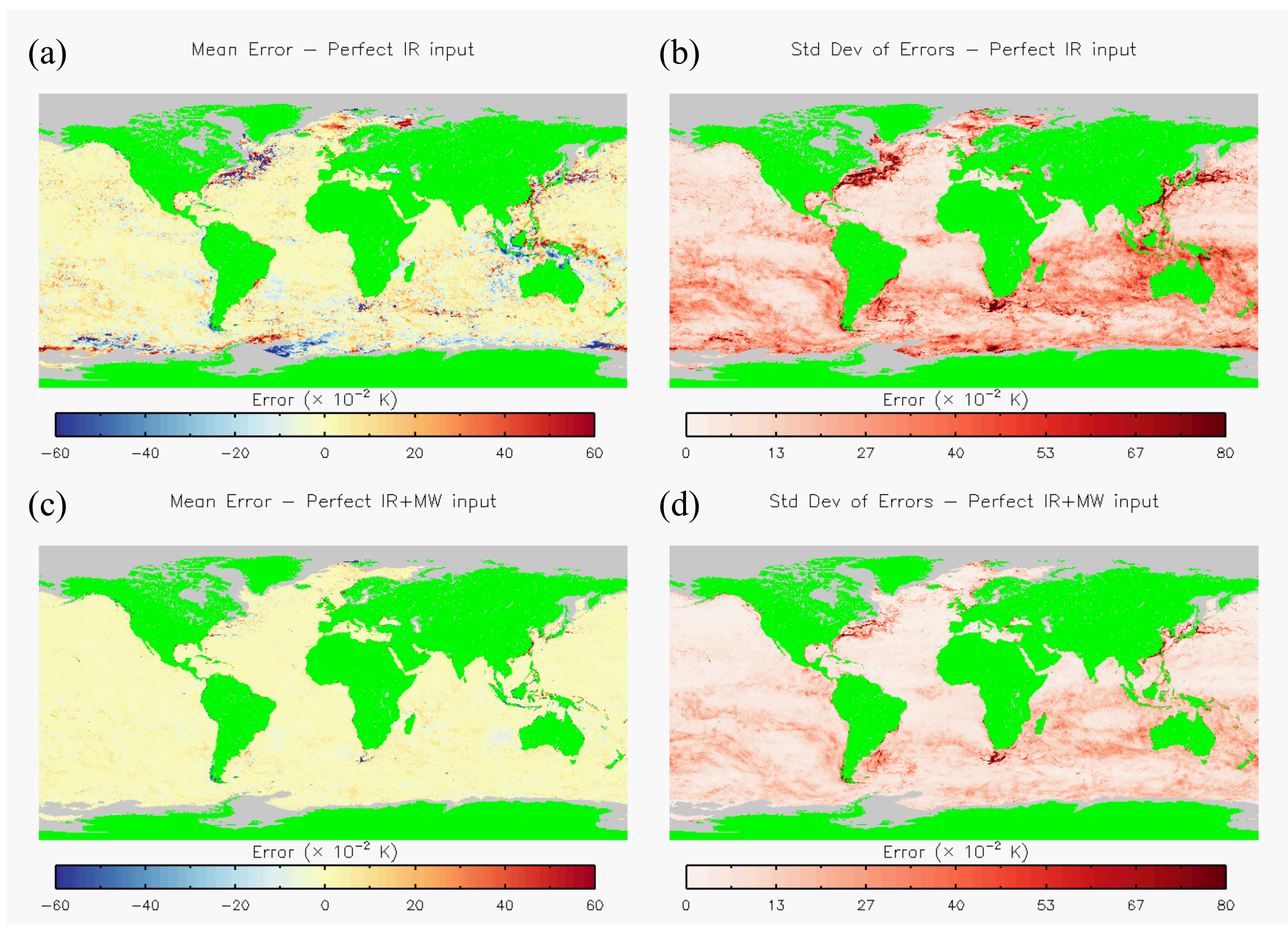
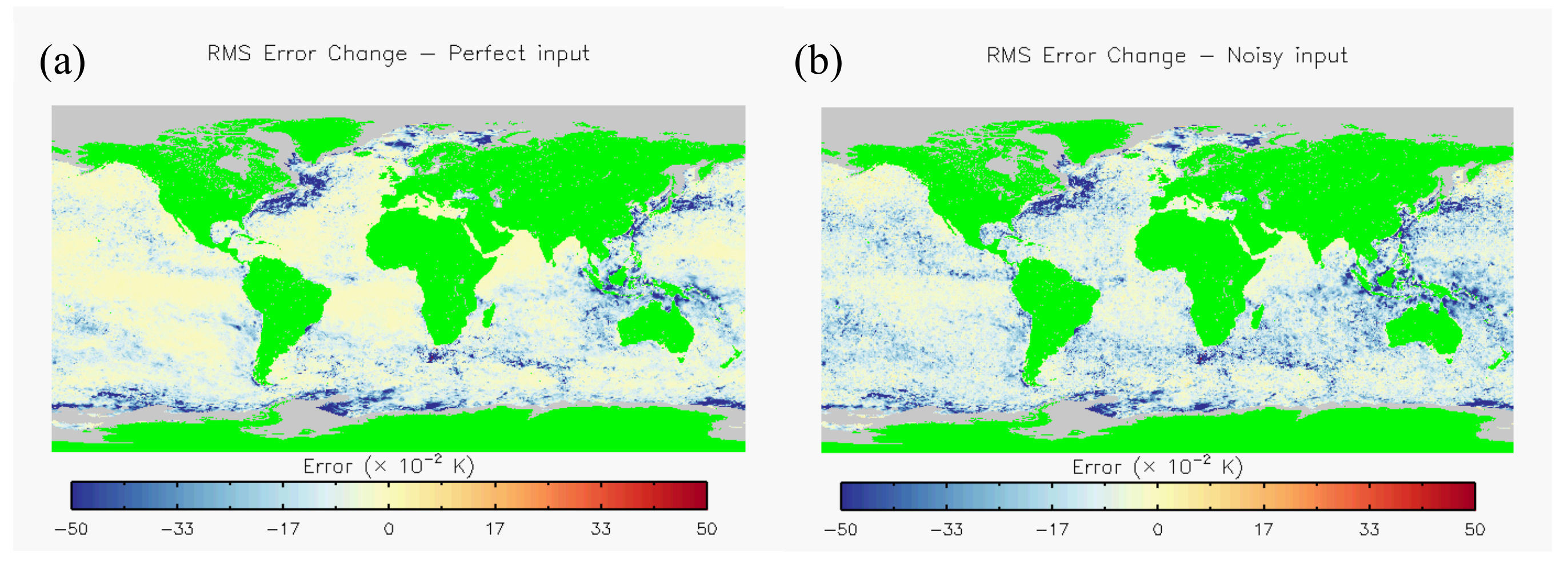
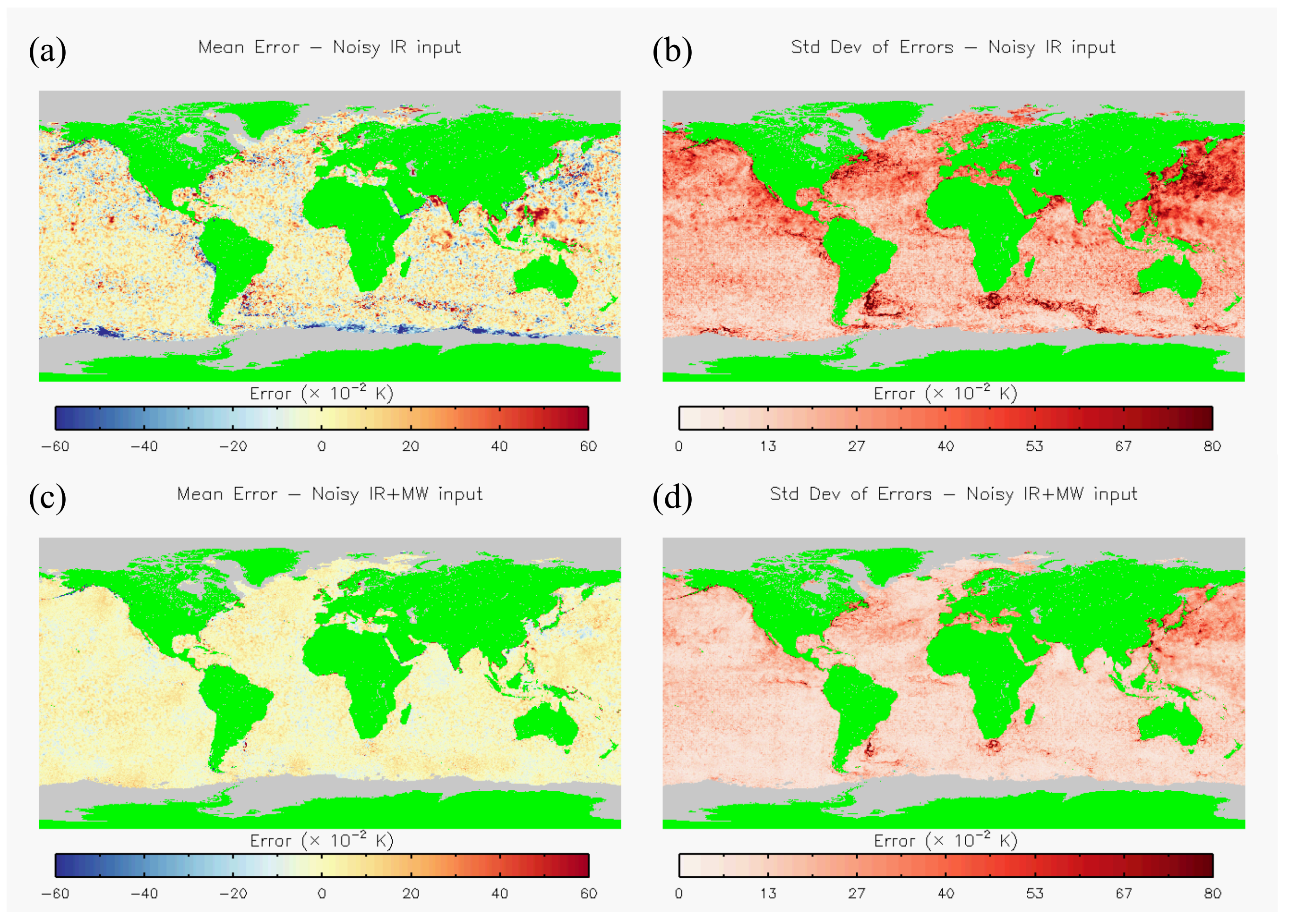
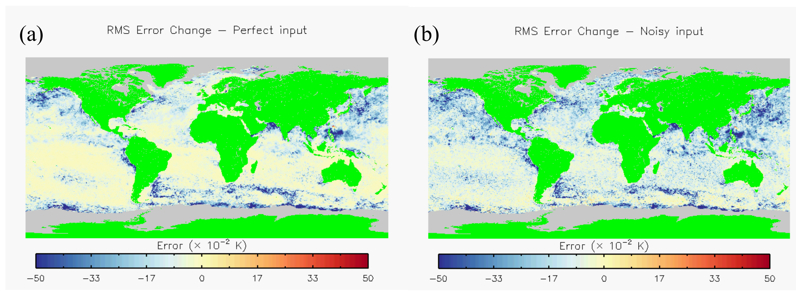
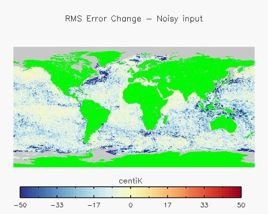
The mean and standard deviation of the error in the daily analysis of the SST were formed via comparison with the original “truth” dataset for the day. Histograms of the distribution and global maps of these statistics are shown for January in Figure 4 and Figure 5, respectively, for the perfect input data cases. Similar comparisons using input data with realistic errors are shown in Figure 6 and Figure 7. The change in the root-mean-square error (RMSE) resulting from the addition of the CIMR data to the analysis inputs is shown in Figure 8. Results for July are similar to those for January and so just the maps of the errors statistics are shown for the data with realistic errors and the change in RMSE in Figure 9 and Figure 10.
Both Figure 4 and Figure 6 show a clear improvement in the error distributions with the addition of the CIMR data and imply an improved ability of the analyses to reproduce the “truth” dataset. As might be expected, the OSTIA analyses in Figure 5, Figure 7 and Figure 9 show patches of larger error standard deviations in regions of dynamical SSTs, such as around the Aghulas Current and the Gulf Stream. More widely, for the infrared-only reconstructions, the error standard deviations appeared to be larger in the southern hemisphere in January and the northern hemisphere in July. This is counter-intuitive as one might expect summer to result in decreased cloudiness and thus improved coverage. In January, for the southern hemisphere, AVHRR and SLSTR had 16.1 ± 0.9% and 14.5 ± 0.9% daily hemisphere coverage, respectively, compared to 11.5 ± 0.8% and 10.1 ± 0.5%, respectively, for the northern hemisphere. However, in July, there was a more mixed coverage picture: 13.0 ± 1.1% and 12.0 ± 0.8% coverage, respectively, for the southern hemisphere compared to 10.8 ± 1.1% and 12.5 ± 1.1%, respectively, for the northern hemisphere. This implied that rather than coverage, the differences in performance between the hemispheres was due to increased variability in summer.
The differences between the northern and southern hemispheres became less pronounced with the addition of the CIMR data. There were still patches of larger RMSE in the dynamical areas even though Figure 7 and Figure 8 show that the biggest improvements from the addition of CIMR data were in these regions. The north-west Pacific in July appeared to remain a difficult region to reconstruct. Close examination shows that the coastal areas had a larger RMSE than the open ocean in all the analyses.
A summary of the RMSE in different regions for each of the configurations is given in Table 2. During validation of current operational OSTIA products, the RMS difference relative to reference observations is typically in the range 0.3–0.5 [14,29], so a similar magnitude of results in this table suggests that this simulation study is performing realistically. The addition of CIMR data resulted in a marked decrease in RMSE in all regions except the coast. The coastal region (defined as cells less than 25 km from land) showed only small improvements with the addition of the CIMR data. This was consistent with the restriction of the PMW observations being greater than this distance from land. The minimisation step in the NEMOVAR algorithm, however, was able to spread some information, spatially accounting for the small improvement. For the case of data with realistic errors, the addition of CIMR data resulted in the global mean RMSE decreasing from 0.369 to 0.210 in January and from 0.395 to 0.249 in July. Improvements of this magnitude in RMSE suggest CIMR should support a step-change improvement in daily SST analyses.

3.2. Reconstruction in Dynamical Regions

Figure 11 shows the spatial power spectra of the SST fields from the January analysis using the data with realistic errors for the Aghulas Current and Gulf Stream regions. These were generated by calculating a fast Fourier transform along the row (constant-latitude) direction of the data in the region. Rows containing any land or sea-ice cells were discarded. The mean transform was found across all the remaining rows and the power was calculated from this in the normal way. The frequency scale was added using a grid cell spacing of 0.05° and the mean latitude of the contributing rows. The resulting spectra are plotted as a ratio to the “truth” power spectra in these regions and so perfect replication of the truth field in these plots would give a ratio of 1:1 across the whole spectrum. In both cases, there was a marked improvement in the agreement with the original “truth” dataset by the addition of the CIMR data, as shown by the blue lines being closer to the 1:1 ratio across almost all spatial frequencies than the red lines.
The structure inherent in the SST fields in these regions is shown in Figure 12. This shows a map of the mean magnitude of the gradient of the SST field in the second half of January. Figure 13 shows the difference from these fields for the reconstructions using the input data with realistic errors. In many instances, these difference maps show pairs of red and blue areas that would be expected from a spatial offset of a feature in the SST field. The area of these regions was greatly reduced by the addition of CIMR data. The fraction of cells where the magnitude of the difference was greater than 0.02 °C∙km−1 decreased from 6.6 % to 3.1% for the Aghulas Current and from 30.2% to 9.8% for the Gulf Stream. In some locations, there were larger patches of difference, e.g., just left of centre in Figure 13a,c and the bottom left of Figure 13b,d. Here, in the IR-only case, the interpolation scheme had produced structures that were not present in the “truth” dataset. These were artefacts resulting from interpolation of data that were too sparse. This limitation of optimal interpolation in regions with strong SST gradients was noted in the context of an AVHRR-only reconstruction by Reynolds et al. [30] and discussed more generally in Reynolds et al. [31]. With the sparser coverage of the IR-only case, the analysis only had intermittent input observations of these structures, i.e., the analysis got to “see” the evolving structures on some days and reconstructed the features only at their locations on those days. The discrete nature of these locations persisted in the time intervals without observations and ultimately became apparent in the mean over the period. The better coverage achieved with CIMR improved the sampling such that there was a more representative set of positions for the structures over the period and thus a better representation of the mean field. These artefactual structures were greatly reduced with the addition of CIMR data because the true structures were sampled at a resolution that usefully resolved their locations on most days.

3.3. Reconstruction of the Southern Ocean and Maritime Continent

Figure 5, Figure 7 and Figure 9 show that the IR-only analysis resulted in biases along the sea-ice edge in the Southern Ocean. Notably, in January, there was a dipole structure to the bias in the region between the Weddell Gyre and Antarctic Circumpolar Current off the tip of the Antarctic Peninsula. This type of structure also occurred less distinctly in the region of the Ross Gyre and the Ross Sea. In July, there was a more uniform cold bias along the ice edge. The additional information provided by the CIMR data was sufficient to eliminate the biases in each of these regions. This was despite the extra masking required around the input data cells that contained sea-ice.
The Maritime Continent also showed a split in the sign of the bias in the IR-only analyses. To the east of this region, these analyses had a warm bias, and to the west, a cold bias. As with the Southern Ocean, this was less pronounced in July with only the eastern warm bias being apparent. There is often significant cloud in both these regions and the improved coverage provided by CIMR resulted in a large improvement in the reliability of the reconstruction.

3.4. Summary

Adding CIMR data to the IR constellation reduced both the mean error and error standard deviation globally. There was also a clear improvement in areas of particular challenge, such as around strong ocean temperature gradients and dynamics and regions of persistent cloud. The “perfect” data results showed that this was a result of the improved coverage available from CIMR despite the lower weight given to each of the individual observations compared to the IR. The fact that this improvement remained when data with realistic errors was used showed that this improvement will hold true when CIMR is added to an IR-only constellation in the future.
In the Southern Ocean, these improvements offer the prospect of greater insights into the Antarctic Circumpolar Current and other currents. Aside from regions with climatologically high amounts of cloud, CIMR observations may also improve the coverage of SST measurements for high-impact events with more transient clouds. For example, the inability of IR instruments to make measurements through clouds resulted in operational OSTIA and other SST products missing the rapid SST drop in the Hurricane Irma event [32]. Although observations from CIMR would still be restricted to rain-free regions, the ability to penetrate clouds means that CIMR has the potential to significantly increase the available observations for such events and thus improve the analysis reconstruction.

4. Conclusions

We have conducted an investigation into the effect of adding CIMR to an IR-only observing system on the global analyses of SST. Adding CIMR resulted in a reduction in the global RMSE of SST in analysis data from 0.37 K to 0.21 K for January and 0.40 K to 0.25 K for July. There were also strong improvements in dynamical regions, such as the Aghulas Current (from 0.59 K to 0.34 K in January and 0.38 K to 0.20 K in July) and Gulf Stream (from 1.29 K to 0.39 K in January and 0.51 K to 0.28 K in July). There were noticeable examples of artefacts in the reconstruction that were removed with the additional coverage provided by CIMR.
CIMR will make an important contribution to global observations of SST and result in a large reduction in the errors in analyses. Its near-daily coverage and ability to provide SST in the presence of clouds will significantly improve the analysis reconstruction of dynamical regions where there are strong SST contrasts and in regions with persistent cloud coverage.

Author Contributions

Conceptualization, C.J.M. and C.D.; methodology, K.P. and C.J.M.; software, K.P., S.G. and O.E.; validation, K.P.; formal analysis, K.P.; investigation, K.P., O.E. and C.P.; resources, C.J.M.; data curation, K.P. and O.E.; writing—original draft preparation, K.P.; writing—review and editing, K.P., S.G., C.J.M. and C.P.; visualization, K.P.; supervision, C.J.M.; project administration, K.P., C.J.M. and C.D.; funding acquisition, C.J.M.

Funding

This research was funded by the European Space Agency under 4000125189/18/NL/AI.

Acknowledgments

The authors thank Adam Blaker and Andrew Coward of the National Oceanography Centre, Southampton, U.K., for access to the model simulations used in this study.

Conflicts of Interest

The authors declare no conflict of interest. The funders commissioned the study and commented on interim results.

References

  1. Clayson, C.A.; Chen, A.D. Sensitivity of a coupled single-column model in the tropics to treatment of the interfacial parameterizations. J. Clim. 2002, 15, 1805–1831. [Google Scholar] [CrossRef]
  2. Webster, P.J.; Clayson, C.A.; Curry, J.A. Clouds, Radiation, and the Diurnal Cycle of Sea Surface Temperature in the Tropical Western Pacific. J. Clim. 1996, 9, 1712–1730. [Google Scholar] [CrossRef]
  3. Chelton, D.B. The Impact of SST Specification on ECMWF Surface Wind Stress Fields in the Eastern Tropical Pacific. J. Clim. 2005, 18, 530–550. [Google Scholar] [CrossRef] [Green Version]
  4. Donlon, C.; Robinson, I.; Casey, K.S.; Vazquez-Cuervo, J.; Armstrong, E.; Arino, O.; Gentemann, C.; May, D.; LeBorgne, P.; Piollé, J.; et al. The Global Ocean Data Assimilation Experiment High-resolution Sea Surface Temperature Pilot Project. Bull. Am. Meteorol. Soc. 2007, 88, 1197–1214. [Google Scholar] [CrossRef]
  5. Nielsen-Englyst, P.; Høyer, J.L.; Toudal Pedersen, L.; Gentemann, C.L.; Alerskans, E.; Block, T.; Donlon, C. Optimal Estimation of Sea Surface Temperature from AMSR-E. Remote Sens. 2018, 10. [Google Scholar] [CrossRef]
  6. Pearson, K.; Gentemann, C.; Kachi, M. Comparison of AMSR2 Sea Surface Temperature Retrievals with In-Situ Data; Group for High Resolution Sea Surface Temperature (ESA/ESTEC): Noordwijk, The Netherlands, 2015; pp. 74–80. [Google Scholar]
  7. Merchant, C.J.; Embury, O.; Bulgin, C.E.; Block, T.; Corlett, G.; Fiedler, E.; Good, S.A.; Mittaz, J.; Rayner, N.; Berry, N.A.; et al. Satellite-based time-series of sea-surface temperature since 1981 for climate applications. Nat. Sci. Data 2019, in press. [Google Scholar]
  8. EU Arctic Policy. Available online: https://eeas.europa.eu/arctic-policy/eu-arctic-policy_en (accessed on 11 June 2019).
  9. Donlon, C. Copernicus Imaging Microwave Radiometer (CIMR)—Mission Requirements Document; ESA-EOPSM-CIMR-MRD-3236; European Space Agency: Katwijk, The Netherlands, 5 March 2019. [Google Scholar]
  10. Donlon, C.J.; Martin, M.; Stark, J.; Roberts-Jones, J.; Fiedler, E.; Wimmer, W. The Operational Sea Surface Temperature and Sea Ice Analysis (OSTIA) system. Remote Sens. Environ. 2012, 116, 140–158. [Google Scholar] [CrossRef]
  11. Donlon, C. Proceedings from the Third GODAE High Resolution SST Pilot Project Workshop; Technical Report No. 16; International GHRSST-PP Project Office: Leicester, UK, 2003. [Google Scholar]
  12. Donlon, C.; Emery, B.; Kawamura, H.; Cummings, J.; Robinson, I.; LeBorgne, P.; May, D.; Minnett, P.; Barton, I.; Rayner, N.; et al. The Recommended GHRSST-PP Data Processing Specification GDS; Technical report No. 17; International GHRSST-PP Project Office: Leicester, UK, 26 March 2004. [Google Scholar]
  13. Mogensen, K.S.; Balmaseda, M.A.; Weaver, A. The NEMOVAR Ocean Data Assimilation System as Implemented in the ECMWF Ocean Analysis for System 4; Technical Report No. 668; European Centre for Medium Range Weather Forecasts: Reading, UK, 2012. [Google Scholar]
  14. Fiedler, E.K.; Mao, C.; Good, S.A.; Water, J.; Martin, M.J. Improvements to feature resolution in the OSTIA sea surface temperature analysis using the NEMOVAR assimilation scheme. Q. J. R. Meteorol. Soc. 2019. [Google Scholar] [CrossRef]
  15. The North Atlantic Climate System Integrated Study. Available online: http://acsis.ac.uk (accessed on 11 June 2019).
  16. Gurvan, M.; Romain, B.-B.; Bouttier, P.-A.; Bricaud, C.; Bruciaferri, D.; Calvert, D.; Chanut, J.; Clementi, E.; Coward, A.; Delrosso, D.; et al. NEMO Ocean Model. In Nemo Ocean Engine; Notes du Pôle de Modélisation de l’Institut Pierre-Simon Laplace (IPSL): Paris, France, 2017. [Google Scholar] [CrossRef]
  17. Madec, G.; Imbard, M. A global ocean mesh to overcome the North Pole singularity. Clim. Dyn. 1996, 12, 381–388. [Google Scholar] [CrossRef]
  18. ORCA Tripolar Grid. Available online: https://www.nemo-ocean.eu/doc/node108.html (accessed on 4 July 2019).
  19. Le Traon, P.Y.; Klein, P.; Hua, B.L.; Dibarboure, G. Do Altimeter Wavenumber Spectra Agree with the Interior or Surface Quasigeostrophic Theory? J. Phys. Oceanogr. 2008, 38, 1137–1142. [Google Scholar] [CrossRef]
  20. Isern-Fontanet, J.; Chapron, B.; Lapeyre, G.; Klein, P. Potential use of microwave sea surface temperatures for the estimation of ocean currents. Geophys. Res. Lett. 2006, 33. [Google Scholar] [CrossRef] [Green Version]
  21. Mackie, S.; Embury, O.; Old, C.; Merchant, C.J.; Francis, P. Generalized Bayesian cloud detection for satellite imagery. Part 1: Technique and validation for night-time imagery over land and sea. Int. J. Remote Sens. 2010, 31, 2573–2594. [Google Scholar] [CrossRef]
  22. Mackie, S.; Merchant, C.J.; Embury, O.; Francis, P. Generalized Bayesian cloud detection for satellite imagery. Part 2: Technique and validation for daytime imagery. Int. J. Remote Sens. 2010, 31, 2595–2621. [Google Scholar] [CrossRef]
  23. Merchant, C.J.; Embury, O.; Roberts-Jones, J.; Fiedler, E.; Bulgin, C.E.; Corlett, G.K.; Good, S.; McLaren, A.; Rayner, N.; Morak-Bozzo, S.; et al. Sea surface temperature datasets for climate applications from Phase 1 of the European Space Agency Climate Change Initiative (SST CCI). Geosci. Data J. 2014, 1, 179–191. [Google Scholar] [CrossRef]
  24. Copernicus Climate Change Service Dataset: Sea Surface Temperature Integrated Climate Data Record (ICDR) from the Advanced Very High Resolution Radiometer (AVHRR), Level 3C (L3C), version 2; Copernicus Climate Change Service: Brussels, Belgium, 2019.
  25. Climate Data Store. Available online: https://cds.climate.copernicus.eu/#!/home (accessed on 8 July 2019).
  26. Rayner, N.; Good, S.A.; Block, T.; Evadzi, P.; Embury, O. SST CCI Product User Guide; Met Office: Exeter, UK, 2019. [Google Scholar]
  27. Bulgin, C.E.; Embury, O.; Corlett, G.; Merchant, C.J. Independent uncertainty estimates for coefficient based sea surface temperature retrieval from the Along-Track Scanning Radiometer instruments. Remote Sens. Environ. 2016, 178, 213–222. [Google Scholar] [CrossRef] [Green Version]
  28. Kilic, L.; Prigent, C.; Aires, F.; Boutin, J.; Heygster, G.; Tonboe, R.T.; Roquet, H.; Jimenez, C.; Donlon, C. Expected Performances of the Copernicus Imaging Microwave Radiometer (CIMR) for an All-Weather and High Spatial Resolution Estimation of Ocean and Sea Ice Parameters. J. Geophys. Res. Oceans 2018, 123, 7564–7580. [Google Scholar] [CrossRef]
  29. Fiedler, E.K.; McLaren, A.; Banzon, V.; Brasnett, B.; Ishizaki, S.; Kennedy, J.; Rayner, N.; Roberts-Jones, J.; Corlett, G.; Merchant, C.J.; et al. Intercomparison of long-term sea surface temperature analyses using the GHRSST Multi-Product Ensemble (GMPE) system. Remote Sens. Environ. 2019, 222, 18–33. [Google Scholar] [CrossRef]
  30. Reynolds, R.W.; Smith, T.M.; Liu, C.; Chelton, D.B.; Casey, K.S.; Schlax, M.G. Daily High-Resolution-Blended Analyses for Sea Surface Temperature. J. Clim. 2007, 20, 5473–5496. [Google Scholar] [CrossRef]
  31. Reynolds, R.W.; Chelton, D.B.; Roberts-Jones, J.; Martin, M.J.; Menemenlis, D.; Merchant, C.J. Objective Determination of Feature Resolution in Two Sea Surface Temperature Analyses. J. Clim. 2013, 26, 2514–2533. [Google Scholar] [CrossRef] [Green Version]
  32. Liu, Y.; Weisberg, R.H.; Law, J.; Huang, B. Evaluation of Satellite-Derived SST Products in Identifying the Rapid Temperature Drop on the West Florida Shelf Associated with Hurricane Irma. Mar. Technol. Soc. J. 2018, 52, 43–50. [Google Scholar] [CrossRef]
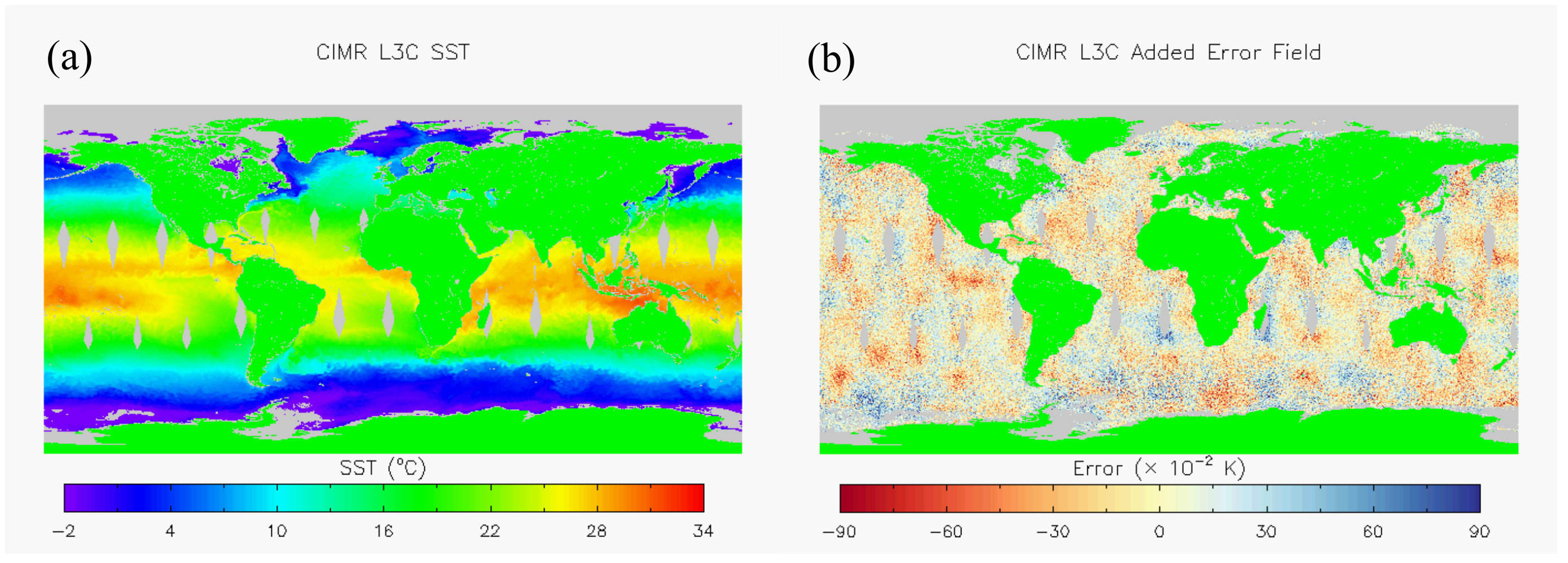
Figure 1. (a) Example of the daily sea surface temperature (SST) field from a Copernicus Imaging Microwave Radiometer (CIMR) level 3 collated (L3C) file and (b) the added error field for this CIMR L3C field.
Remotesensing 11 02362 g001
Figure 2. Processing steps involved in generating the synthetic CIMR data.
Remotesensing 11 02362 g002
Figure 3. Processing steps involved in creating synthetic SST data for the Advanced Very High Resolution Radiometer (AVHRR) and the Sea and Land Surface Temperature Radiometer (SLSTR). The data generation made use of the Generalised Bayesian Cloud Screening (GBCS) processor and the Operational Sea Surface Temperature and Sea Ice Analysis (OSTIA) system.
Remotesensing 11 02362 g003
Figure 4. Statistics of the differences between the analysis of January SST fields and original “truth” SST for infrared-only (IR-only) (red) and combined infrared (IR) and microwave (MW) (blue) input data: (a) mean error for perfect input and (b) standard deviation of the error for perfect input.
Remotesensing 11 02362 g004
Figure 5. Maps of the January error statistics: (a) mean error with perfect IR data only, (b) standard deviation of the error with perfect IR data only, (c) mean error with combined perfect IR and CIMR data and (d) standard deviation of the error with combined perfect IR and CIMR data..
Remotesensing 11 02362 g005
Figure 6. Statistics of the differences between the analysis of January SST fields and the original “truth” SST for IR-only (red) and combined IR and MW (blue) input data with realistic errors: (a) mean error and (b) standard deviation of the error.
Remotesensing 11 02362 g006
Figure 7. Maps of the error statistics during January for input data with realistic errors: (a) mean error with IR data only, (b) standard deviation of the error with IR data only, (c) mean error with combined IR and CIMR data and (d) standard deviation of the error with combined IR and CIMR data.
Remotesensing 11 02362 g007
Figure 8. Change in the RMS error of the reconstructed SST field in January from adding CIMR data to the input for: (a) perfect input data and (b) input data containing realistic errors.
Remotesensing 11 02362 g008
Figure 9. Maps of the error statistics during July for input data with realistic errors: (a) mean error with IR data only, (b) standard deviation of the error with IR data only, (c) mean error with combined IR and CIMR data and (d) standard deviation of the error with combined IR and CIMR data.
Remotesensing 11 02362 g009
Figure 10. Change in the RMS error of the reconstructed SST field in July from adding CIMR data to the input for: (a) perfect input data and (b) input data containing realistic errors.
Remotesensing 11 02362 g010
Figure 11. Comparison of the power spectra of the SST field in January from IR-only analysis (red) and combined IR and MW analysis (blue) where both contain realistic input errors. The data are plotted as a ratio to the “truth” SST power spectrum at each wavelength: (a) Aghulas Current region and (b) Gulf Stream region.
Remotesensing 11 02362 g011
Figure 12. Gradient of the SST field in January in the “truth” data set for: (a) Aghulas Current region and (b) Gulf Stream region.
Remotesensing 11 02362 g012
Figure 13. Difference from the “truth” SST gradient field in January for the output of OSTIA reconstructions using input data with realistic errors: (a) IR-only data for the Aghulas Current region, (b) IR-only data for the Gulf Stream region, (c) combined IR and MW data for the Aghulas Current region and (d) combined IR and MW data for the Gulf Stream region.
Remotesensing 11 02362 g013
Table 1. Uncertainty components for each of the CIMR channels. The columns give the total uncertainty, as well as the radiometric, orbital stability, lifetime-stability and pre-launch calibration contributions to the total uncertainty budget.
Channel (GHz)UtotalUNEΔTUorb-stabUlife-stabUpl-cal
1.410.50.30.20.20.2
6.90.40.20.10.20.2
10.650.450.30.10.20.2
18.70.60.40.20.20.2
36.50.80.70.20.20.2
Table 2. Root-mean-square error in different regions for the various experimental configurations.
ConfigurationGlobalAghulas CurrentGulf StreamMaritimeSouthern OceanCoast
JanPerfect IR-only0.3100.5321.2860.3940.3690.641
Perfect IR + CIMR0.1750.3120.3580.2120.1320.608
Realistic IR-only0.3690.5871.2890.4620.3960.667
Realistic IR + CIMR0.2100.3370.3860.2330.1690.622
JulyPerfect IR-only0.3380.3250.4100.2360.4930.981
Perfect IR + CIMR0.2250.1590.2580.1590.0780.969
Realistic IR-only0.3950.3840.5060.3350.4960.995
Realistic IR + CIMR0.2490.1990.2840.2000.1300.969