Article

Monitoring of Urbanization and Analysis of Environmental Impact in Stockholm with Sentinel-2A and SPOT-5 Multispectral Data

Division of Geoinformatics, Department of Urban Planning & Environment, Royal Institute of Technology, Teknikringen 10A, 10044 Stockholm, Sweden
*
Author to whom correspondence should be addressed.
Remote Sens. 2019, 11(20), 2408; https://doi.org/10.3390/rs11202408
Submission received: 7 August 2019 / Revised: 9 October 2019 / Accepted: 15 October 2019 / Published: 17 October 2019
(This article belongs to the Special Issue Mapping Ecosystem Services Flows and Dynamics Using Remote Sensing)

Abstract

:
There has been substantial urban growth in Stockholm, Sweden, the fastest-growing capital in Europe. The intensifying urbanization poses challenges for environmental management and sustainable development. Using Sentinel-2 and SPOT-5 imagery, this research investigates the evolution of land-cover change in Stockholm County between 2005 and 2015, and evaluates urban growth impact on protected green areas, green infrastructure and urban ecosystem service provision. One scene of 2015 Sentinel-2A multispectral instrument (MSI) and 10 scenes of 2005 SPOT-5 high-resolution instruments (HRI) imagery over Stockholm County are classified into 10 land-cover categories using object-based image analysis and a support vector machine algorithm with spectral, textural and geometric features. Reaching accuracies of approximately 90%, the classifications are then analyzed to determine impact of urban growth in Stockholm between 2005 and 2015, including land-cover change statistics, landscape-level urban ecosystem service provision bundle changes and evaluation of regional and local impact on legislatively protected areas as well as ecologically significant green infrastructure networks. The results indicate that urban areas increased by 15%, while non-urban land cover decreased by 4%. In terms of ecosystem services, changes in proximity of forest and low-density built-up areas were the main cause of lowered provision of temperature regulation, air purification and noise reduction. There was a decadal ecosystem service loss of 4.6 million USD (2015 exchange rate). Urban areas within a 200 m buffer zone around the Swedish environmental protection agency’s nature reserves increased 16%, with examples of urban areas constructed along nature reserve boundaries. Urban expansion overlapped the deciduous ecological corridor network and green wedge/core areas to a small but increasing degree, often in close proximity to weak but important green links in the landscape. Given these findings, increased conservation/restoration focus on the region’s green weak links is recommended.

Graphical Abstract

1. Introduction

As of 2018, 55% of the world population resides in urban areas, a percentage that is projected to increase to 68% by 2050 [1]. Increasing urbanization poses challenges for sustainable development, not least in regard to environmental management. Urbanization results in changes in land cover, hydrological systems, biogeochemistry, climate and biodiversity. Worldwide, urban expansion is one of the primary drivers of habitat loss and species extinction [2,3]. Urbanization has a two-fold effect on surrounding remaining natural land cover: (1) Growing urban areas lead to increased demand for resources/energy from natural areas and increased amounts of emissions/waste for the natural environment to regulate and (2) construction of urban areas leads to fragmentation, isolation and loss of natural and semi-natural land cover [4,5]. Urban development changes microclimate and air quality [6], habitat structure and patterns of species diversity and abundance [7,8,9] as well as the availability of natural resources [10]. It also affects nutrient cycling [11], hydrological function [12], primary productivity [13] and ecosystem dynamics [4,14]. Thus monitoring changes in landscape patterns and its influence on ecosystem services is crucial to sustainable urban planning and development.
The UN’s Sustainable Development Goals (SDGs) provide a blueprint for action in achieving social, economic and environmental sustainability around the world. SDG 15 Life on Land, which aims to “protect, restore and promote sustainable use of terrestrial ecosystems, sustainably manage forests, combat desertification, and halt and reverse land degradation and halt biodiversity loss” [15], stands out as particularly relevant to the environmental challenge posed by urbanization. The first SDG 15 target is to “By 2020, ensure the conservation, restoration and sustainable use of terrestrial and inland freshwater ecosystems and their services, in particular forests, wetlands, mountains and drylands, in line with obligations under international agreements” (15.1). Yet UN-DESA’s expert group meeting on progress towards SDG 15 which took place in May 2018 noted that there has been progress in indicators related to actions (e.g., numbers of protected areas), but not status (e.g., state of species). More specifically, they state that “the monitoring framework… does not capture essential elements related to quality… pointing to the need for additional indicators in areas such as forest intactness [and] management effectiveness of protected areas” [16]. Thus, there is a clear need for methodology to assess the status of protected areas and forests as a means of evaluating their maintenance, restoration and sustainable use. The UN-DESA expert group meeting also noted the usefulness of a landscape-level approach to achieve sustainability. This research offers a regional case study in monitoring environmental impact from urban expansion, particularly in proximity to protected areas, which can provide valuable information on the status of forests and other natural land-cover types necessary for maintaining ecosystem function and services and thereby assist in evaluating progress towards SDG target 15.1 as well as relevant national goals.
Over the past few decades, there has been substantial urban growth in Stockholm, Sweden, now the largest city in Scandinavia. Growth in the area is due mainly to the increasing population, which rose by 22% between 2000 and 2015. Urbanization is placing pressure on the natural environment in and around Stockholm, which contains a number of protected areas as well as “green wedges” crucial to providing many of the region’s ecosystem services. It is therefore important to map urban land-cover changes and assess the environmental impact of these changes in a timely and accurate manner. The Swedish government recently took steps to ensure sustainable management of its green and blue resources in urban areas by requiring all counties to draw up regional action plans for their green infrastructure. But Stockholm planning authorities have limited quantitative information concerning the impact of urban growth on green infrastructure for the entire county in recent decades. This research investigates and evaluates the evolution of land-cover change in Stockholm County between 2005 and 2015 with a particular focus on what impact urban growth has had on protected green areas, green infrastructure and urban ecosystem service provision.
While methods for mapping and monitoring of urban land-cover change from satellite data have been developed extensively in recent decades [17,18], ESA’s Sentinel-2A Multispectral Instrument (MSI) data provides new opportunities for urban land-cover classification thanks to its higher spatial and spectral resolutions in comparison to the oft used Landsat program [19]. Classification and comparison of Sentinel-2A data with historical satellite data at a similar spatial resolution, such as SPOT-5 (Satellite Pour l’Observation de la Terre), appear as a promising new area for investigation and evaluation of spatio-temporal environmental changes in urban areas. So far, only one study was found in the literature using Sentinel-2A and SPOT data to monitor urban expansion and green space change with a pixel-based hybrid classifier by combining traditional unsupervised (self-organizing data analysis technique algorithm) and supervised (maximum likelihood) classification [20]. No study has been conducted to provide a comprehensive analysis of environmental impact of urbanization using such datasets. Recently, a new approach for appraisal of ecosystem services in urban areas was developed by extending the ecosystem service concept through the integration of spatial characteristics of ecosystem service provisional patches via landscape metrics [21]. These ecosystem service provision bundles have been tested based on Sentinel-2A MSI data in Beijing, a rapidly urbanizing metropolitan area [21] but not in a moderately urbanizing region such as Stockholm, where there is a need for information on more recent urban expansion and resulting impact on green structure and ecosystem services [22].
The objectives of this research are therefore to investigate the extent and nature of land-cover change in Stockholm between 2005 and 2015 based on object-oriented support vector machine (SVM) classifications of Sentinel-2A MSI and SPOT-5 high-resolution instruments (HRI) satellite data, and to estimate this change’s impact on and relation to legislatively protected and ecologically significant areas of green infrastructure as well as to assess urban ecosystem service provision bundle changes at the landscape level. This is a complementary dual-level analysis approach: At the landscape regional level, yielding an estimation of overall impacts on ecosystem service provision for the whole region, combined with more specific analysis pertaining to green infrastructure that transcends administrative boundaries and highlights potentially problematic areas, which are localized manifestations of the regional trends. This kind of information can assist policymakers and planners in Stockholm in making both local and regional decisions about future urban development and environmental protection or mitigating measures. This methodological approach can also serve as an informative case study for other cities/countries considering methods for evaluating their progress towards UN SDG target 15.1 and other national environmental policy aims.

2. Related Literature

2.1. Urban Land-Cover Mapping Based on Optical Remote Sensing Data

Remote sensing data provides valuable geographic information given its spatially consistent geometric detail provided at high temporal frequency [23] and the mapping and monitoring of urban land-cover change based on remote sensing data have been developed extensively in recent decades. Urban environments pose a unique challenge for mapping and classification given the increased complexity of land-cover features found within them, particularly at higher spatial resolutions [24,25,26].
Land-cover mapping of urban areas with medium- to high-resolution satellite data has been successfully performed at local and regional scales, most often based on optical data from satellites such as Landsat, SPOT, Aster, Ikonos or QuickBird [25,27,28,29,30]. In comparison to other pixel-based classification methods, object-based image analysis (OBIA) has consistently returned superior results in land-cover classification accuracy thanks to its use of contextual information such as shape, texture and neighborhood information in addition to spectral data [31]. Powers et al. [32] tested the performance of OBIA classification by resampling images to different spatial resolutions (5, 10, 15, 20, 25 and 30 m) and found that 10 m yielded the highest classification accuracy. Indeed, 10 m resolution SPOT imagery has been used successfully to obtain high accuracy urban land-cover maps, particularly in combination with OBIA techniques [29,33,34,35]. Very high resolution (VHR) data, such as Ikonos or QuickBird, has also proven useful in the classification of detailed urban land-cover maps, but has been less utilized due to its often commercial nature, limited geographical coverage and demand for computational and storage resources [36].
In their review of supervised object-based land-cover image classification, Ma et al. [24] found that SPOT data provided the highest accuracy of all sensor types tested with the exception of unmanned aerial vehicles and that the random forest and support vector machine (SVM) supervised classifiers yielded the highest mean classification accuracies. They note that some uncertainties still exist with regard to feature selection in the process of SVM classification but that previous research suggests that higher accuracy occurs when the number of features is less than 30 [37,38]. SVM is particularly effective for classification of high-dimensional or multi-source data [39,40]. Moving from pixel-based techniques towards object-based representation, the dimensions of remote sensing imagery feature space increases significantly. This results in increased complexity of the classification process. Non-parametric classifiers like SVM often provide better results in complex landscapes and are more suitable when using non-spectral data in classification since there is no assumption of normal data distribution [36]. The superiority of SVM to other classifiers in object-based classification has been reported by various studies, e.g., [39,41].
Recent research highlights the advantages of the use of Sentinel-2 imagery for urban land-cover classification. Pesaresi et al. [19] found that the higher resolution and thematic content of Sentinel-2 data were better suited to detecting built-up areas than Landsat imagery. The findings of Momeni et al. [42] suggest that, where VHR data is not available, the advanced spectral capabilities of recent sensors like Sentinel-2 combined with OBIA and an SVM classifier hold potential for high accuracy mapping of complex urban land cover. The research of Thanh Noi and Kappas [43] confirms that the SVM classifier performs better (higher accuracy and less sensitivity to training sample sizes) than either random forest or k-nearest neighbor when applied to Sentinel-2 data. Given these research findings, an OBIA approach combined with the SVM classifier was chosen as a promising and reliable method with which to produce urban land-cover maps from both SPOT-5 HRI and Sentinel-2A MSI data at different points in time in order to make spatio-temporal comparisons and evaluate environmental impact.

2.2. Urban Environmental Impact Analysis

Anthropogenic influence and impact on the condition and quality of natural and semi-natural environments have increasingly been assessed and presented in terms of ecosystem services, which can be defined as the benefits that humans derive from ecosystems [44]. Urban expansion and the resulting land-cover conversion and fragmentation often negatively affect biodiversity and ecosystem function and services [45,46,47,48,49]. While remote sensing has increasingly contributed to ecosystem service assessments in general [50,51,52], it has been less frequently used to assess urban ecosystem service changes apart from economic valuation schemes, e.g., [53]. Urban ecosystem services, such as air filtration, microclimate regulation, water regulation, waste treatment and recreational/cultural values, are important because of their direct effects on human health and security [54,55]. Changes in the spatial attributes of ecosystem service-providing land cover, such as green infrastructure, in urban areas have not often been examined and there is opportunity for further research in this area [21,56]. Multitemporal remote sensing-based urban land-cover classifications provide a basis for assessment of these environmental spatial changes and their influence on ecosystem service provision.
Since landscape pattern influences the functioning and provision of ecosystem services [47,57,58], changes in spatial pattern quantified by landscape metrics can act as indicators of impact on ecosystem services [56,59]. Landscape metrics have an established record as tools to measure spatial heterogeneity in landscapes [60,61,62,63] and have been used to estimate fragmentation in urbanizing landscapes [64,65,66,67]. Lausch et al. [68] have found that high hemeroby (low naturalness and high human pressure on landscapes) reduces heterogeneity in space and time within patterns and the patch matrix model, which constitutes the framework for calculation of landscape metrics, is recommended for analysis of these kinds of, most notably urban, landscapes.
Haas and Ban [21] recently used landscape metrics in the construction of urban ecosystem service provision bundles to assess the environmental impact of urban growth in Beijing, China between 2005 and 2015, and their incorporation of landscape metrics added a clear spatial component which is important but often lacking in evaluation of changes in ecosystem services [56,69,70]. Their analysis was based on classifications of Landsat and Sentinel-2A data which have differing spatial resolutions (30 m vs. 20/10 m respectively) and as a result, the high-resolution information from Sentinel-2A sensors could not be fully utilized in the metric-based ecosystem service assessment. Wetlands, which play a significant role in the provision of ecosystem services especially in proximity to urban areas [55,71], were also notably absent in their study area. Application of their methodology in a very different urbanizing region such as Stockholm, Sweden, which includes a number of wetlands, and comparison of results from Sentinel-2A with higher resolution SPOT data over the same time period is of interest for evaluating the method’s full potential as well as its sensitivity and transferability.

2.3. Stockholm Green Infrastructure Change Monitoring

As part of the global Millennium Ecosystem Assessment, the Stockholm Urban Assessment (SUA) [72] was selected as a sub-global assessment example, and the main objective of more recent SUA research is to raise awareness among planners and policymakers of the role that Stockholm green structure plays in generating ecosystem services. Both the SUA and its revisitation in 2013 were based on a study area that encompasses the urban metropolitan core of Stockholm but that represents only 15% of the total land area of Stockholm County [22]. While there is considerable political will to preserve green structure in the Stockholm region, both studies state that it continues to be steadily reduced and fragmented by urban expansion. Colding [22] acknowledges that there is a lack of data on how much green structure has been lost in the most recent decades (i.e., since the 1990s) and Colding et al. [72] and Borgström [73] have emphasized the importance of shifting the management/research perspective from the local to the regional landscape scale. Hence there is a need for recent and reliable information on urban expansion-induced loss of green structure in Stockholm County as a whole.
In response to the Swedish government’s recently adopted requirements regarding planning for green infrastructure, the Stockholm County Administrative Board (SCAB) has drafted a green infrastructure action plan. One of the key considerations when it comes to evaluating and planning for Stockholm’s green infrastructure is change in relation to forests, specifically the loss of valuable core areas or important links due to clear cuts or exploitation [74]. Analysis of core areas and ecological corridors for both coniferous/mixed and broadleaved/deciduous forests was performed [75] as a basis for recommendations pertaining to forested areas. In the new regional development plan produced by the Stockholm County Growth and Regional Planning Administration (TRF) in 2018, a network of 10 green wedges, which follow the urban structure from the outskirts of the metropolitan area in towards the center of Stockholm, represents the region’s green infrastructure. These large green areas provide flora and fauna with habitat and the possibility of dispersal as well as many of the region’s ecosystem services [76]. Much of the planning process in the Stockholm region takes place on the municipal level but municipalities often have difficulty in obtaining a clear, holistic picture of factors that cross city boundaries, which often do not coincide with ecoregion boundaries. The regional action plan points out specifically that green connections and valuable areas that cross municipal boundaries need to receive more planning attention so that the functions and value of the green wedges, in particular, do not disappear [74]. Comparison of classified remotely sensed urban land-cover data with administrative boundaries and significant green infrastructure can reveal these transboundary “hotspots.” This research highlights local areas of environmental impact where the territory of several municipalities is involved and where transboundary collaboration is likely needed to sufficiently address potential threats and/or problems.
While it does not develop new image processing techniques, the focus and uniqueness of this research is to “operationalize” the integration of recent data and techniques from the fields of remote sensing and landscape ecology to support sustainable urban planning, and specifically for the monitoring of ecosystem services at the landscape level and nature reserves on a more localized level. These are two complementary and important planning levels: landscape trends of urban impact on ecosystem service provision as well as localized urban impacts on ecologically important regional green infrastructure, which are not often possible to combine in a single methodological study. It also meets the need as expressed by researchers and planning authorities in Stockholm for comparative historical urban growth data and the possibility to obtain a geographic overview that transcends administrative boundaries when observing changes to green infrastructure. The opportunity to test the use of relatively new higher resolution Sentinel-2A MSI data in urban land-cover classification, to utilize the classifications to further investigate effectiveness of ecosystem service bundles in estimating urban impact on ecosystem service provision in a moderately growing urban environment, and the need for monitoring methodology and evaluation of protected areas in urban environments as laid out in SDG 15.1 also motivate this research.

3. Study Area and Data Description

3.1. Study Area

Stockholm municipality covers a land area of around 188 km², while Stockholm County covers 6519 km² [77]. The first to receive the Green Capital Award from the European Union in 2010, Stockholm is often cited as a city that leads in sustainable urban development and in preserving the balance between its green and built-up spaces [78,79]. Yet the region’s population is continually growing, placing pressure on the natural environment and increasing demand for built-up areas. The regional planning authorities have a goal of creating 22,000 new dwellings each year up to 2030 [76]. This study investigates how green areas have been impacted by urban expansion in Stockholm County between 2005 and 2015.
The study area is Stockholm County which contains 26 municipalities including Stockholm city (see Figure 1). The total area included in the analysis of this study is approximately 13,790 km2, of which land area is approximately 6690 km2. The major land-cover classes in the region are high-density residential/commercial built-up areas (HDB), roads/railway, low-density built-up areas (LDB), urban green space, golf courses, forest, agriculture, bare rock/clear cut areas, wetlands and water.
Some of the above-mentioned land-cover classes can benefit from further explanation, while the others are more self-evident. The HDB class is somewhat unique in this study since much of the “high density built-up” areas in the city center of Stockholm are composed of buildings that have businesses on the ground floor but residences on the upper floors. The HDB areas classified in the center of Stockholm do therefore include some commercial areas, which could at the same time be considered residential. HDB in this study over Stockholm County also includes industrial, commercial or construction areas such as industrial parks or shopping centers more likely to be found on the outskirts of urban areas. The roads/railway class also includes airport runways. The LDB land-cover class for Stockholm is characterized by suburban residential areas with vegetation around or between buildings. Prime examples of urban green space are city parks or sports fields, but the class also includes any otherwise undesignated green areas in or around urban areas. The eastern part of the Stockholm County region is characterized by the archipelago with its more than 30,000 islands. Stockholm City itself is partially built on a group of islands. Thus, part of the natural geomorphology of this region includes the frequent occurrence of bare rock outcroppings, especially along the coast. The bare rock/clear cut class takes into account these outcroppings as well as clear cut formerly forested areas that often expose a mix of the bare rock/soil land surface underneath.

3.2. Data Description

A single Sentinel-2A MSI image at product level 1C captured on August 23, 2015, was acquired and used in classification. It has less than 1% cloud coverage and provides spectral data over the majority of the geographic area of Stockholm County. It was necessary to acquire ten scenes of SPOT-5 HRI imagery at product level 1A in order to cover the whole of Stockholm County. For some sections of the county over which no suitable imagery from 2005 could be found, good quality SPOT imagery from the summer months of the closest year possible were used. The dates of the ten images are as follows: 16 June 2005 (two images), 2 July 2005 (one image), 11 July 2005 (one image), 2 September 2005 (one image), 5 August 2006 (one image), 23 May 2007 (one image), 4 June 2008 (two images) and 19 September 2008 (one image). The 2005 imagery covers approximately 50% of the study area, 2006 and 2007 imagery cover about 10% each and the imagery from 2008 covers roughly 30%.
The images were selected from the full vegetation growth season to maximize the spectral differences between built-up areas and vegetation and to thereby reduce detection of unreal changes caused by seasonal differences between years. The Sentinel-2 MSI and SPOT-5 HRI bands used in this study and their characteristics are listed in Table 1. All SPOT-5 bands were used for segmentation and classification. For Sentinel-2, Bands 5, 6, 7, 8a, 11 and 12 were pan-sharpened to 10 m [80] in order to perform the segmentation using all the bands at the same resolution. This procedure can increase the spectral consistency of the image segments and improve the overall accuracy [81].

4. Methodology

4.1. Image Pre-Processing

An overview of this study’s methodology is presented in Figure 2. Sentinel-2 Level 1C images are radiometrically and geometrically correct including ortho-rectification and spatial registration on a global reference system with sub-pixel accuracy [82].
Since level 1A processing of SPOT imagery includes radiometric but not geometric correction, it was necessary to orthorectify each of the 10 SPOT images to the Sentinel-2A image. This was done using GSD-Elevation data, grid 50+ nh, a national elevation model in grid form with two decimal height values and 50 m resolution [83], and the rational polynomial coefficients (RPC) provided within the image metadata. The average RMS errors were 0.3 and 0.25 pixels for the X and Y coordinates respectively. The images were then mosaicked to create one scene over the entire county. The above pre-processing steps were performed using PCI Geomatica software.

4.2. Segmentation and Classification of Satellite Data

Segmentation, feature extraction and classification of the two sets of images were performed using eCognition Developer software [84]. Bands 1–8a, 11 and 12 from Sentinel-2A and all four SPOT-5 bands were used in segmentation and classification. For segmentation, scale parameters of 15 for 2005 and 50 for 2015 were used and homogeneity criteria were set at 0.1 for shape and 0.5 for compactness for 2005 and 0.7 for both criteria for 2015. These parameters were selected based on trials and provided the most appropriate objects for classification in that they most closely represented discrete areas of different land-cover types and shapes in the images. A larger-scale parameter and resulting segments for 2015 were necessary in order to distinguish LDB from UGS; smaller segments placed too much UGS within LDB areas. The 2005 data required a smaller scale parameter and segments since it is a mosaic of 10 images with more variance in spectral qualities of objects, hence smaller “purer” objects yielded better classification results.
Training samples were gathered for 19 different classes initially: 4 for HDB, 1 for LDB, 3 for roads, rail and runway, 3 for UGS, 1 for golf courses, 2 for agriculture, 2 for forest, 1 for water, 1 for bare rock/clear cuts and 1 for wetlands. The classes were then aggregated following classification. The SVM algorithm was used to classify the selected spectral, texture and shape features. As the data is parametric, the linear kernel was chosen to avoid over-fitting. Mean and standard deviation of the above-mentioned spectral bands were used and the shape features included were asymmetry, roundness and rectangular fit. Based on trials, it was found the gray-level difference vector (GLDV) entropy (all directions) texture feature contributed to the best classification results, more so than multiple gray-level co-occurrence matrix (GLCM) features. The texture was included since previous studies have shown that texture measures such as GLCM can improve the classification accuracy of optical medium- to high-resolution satellite imagery [66,85,86,87].
To further improve the classification results, ancillary data and a set of rural masks were used to reclassify noted problematic areas. Roads misclassified as HDB and LDB were corrected using an asymmetry threshold and wetlands were corrected according to a water proximity threshold. Erroneous occurrences of agriculture in and around urban areas were corrected using Statistics Sweden’s 2010 densely populated area (tätort) geodata set [88] and re-assigned to UGS. An agricultural mask was used to correct over-assignment of UGS and golf courses in rural areas. To correct assignments of HDB in the Stockholm archipelago, data from the DMSP-OLS radiance calibrated nighttime lights time series [89] were used to re-classify HDB in dark areas to bare rock. An archipelago mask was also used to correct the over-assignment of wetlands and agricultural areas to bare rock. Once the segmentation-based SVM classifications of the two sets of imagery and post-classification corrections were completed, accuracy assessments were performed using at least 1000 validation sample vector points for each land-cover class.

4.3. Methods for Landscape Change Analysis

Two complementary methods for landscape change analysis were employed in this study. First, in order to give a landscape perspective overview of change to regional ecosystem services, selected landscape metrics were derived and used to construct urban ecosystem service bundles, thereby including spatial characteristics of the provisioning classes in change estimation. The second method focuses on more specific and localized changes in urban areas and green structure on administrative levels within Stockholm County as well as around the region’s legislatively protected and ecologically significant areas.

4.3.1. Landscape Metrics and Urban Ecosystem Service Bundles

Haas and Ban [21] recently incorporated landscape metrics in the construction of urban ecosystem service provision bundles, adding a clear spatial component that is important but often lacking in the evaluation of changes in ecosystem services [56,69,70]. Their methodology is here adapted and applied to the Stockholm County landscape. Change in these bundles can reveal how ecosystem service provision in and around Stockholm has been impacted by urban expansion between 2005 and 2015.
In regard to the Stockholm region’s urban ecosystem services, Bolund and Hunhammar [55] identified a number of these, including air filtration, rainwater drainage, microclimate regulation, noise reduction, waste treatment and recreational/cultural values. Other services important in Stockholm County are described more generally in the County’s draft green infrastructure action plan [74]. This information informed the selection of ecosystem services for evaluation listed in Table I, which include 2 provisioning, 7 regulating, 1 supporting, 1 combined regulating/supporting and 4 cultural services. Identification of the provisioning land-cover classes for each of these services is based on the urban ecosystem services summary by Gomez-Baggethun et al. [54].
Influential spatial attributes for these ecosystem services and metrics to quantify them were proposed by Haas and Ban [21]. Based on the work of [9,48,54,58,59,90] among others, they defined service provision dependencies on spatial attributes in the following way, with the exception of the diversity criterion which has here been adapted to the Stockholm context:
  • Area: Larger green/blue areas provide more ecosystem services;
  • Connectivity: Connected green/blue areas within landscapes increase service provision through enhanced movement corridors and material flows;
  • Core: Core patch areas with no edge influence are important for species through the provision of a more unaltered habitat;
  • Diversity: Increasing diversity in a heretofore predominantly green/blue landscape (such as Stockholm County) decreases services through the shift towards larger or more numerous and therefore more influential urban patches;
  • Edge: Edge contamination of natural blue and green spaces through built-up space affects service quality though pollution and decreased species movement;
  • Proximity: Closeness to built-up areas increases service provision importance.
These distinct but complementary spatial attributes for ecosystem service provision provide the theoretical basis for the selection of the landscape metrics to be calculated, which is a key step in the construction of the ecosystem service bundles. The appropriate landscape metrics to measure these attributes are listed in Table 2 and defined below. They are the same as those used by Haas and Ban [21] with the exception of one: PLAND. The majority are described according to McGarigal et al. [90] and adapted to the Stockholm context:
  • CA: Class area measures landscape composition; specifically, how much of a landscape is comprised of a particular patch type;
  • COHESION: The patch cohesion index measures the physical connectedness of the considered patch type. Patch cohesion increases as the patch type becomes more consolidated or aggregated in its distribution, and thus more physically connected;
  • CWED: Contrast-weighted edge density is an index that takes into account both edge density and edge contrast. It standardizes edge to a per unit area basis that facilitates comparison among landscapes of various sizes. Edge contrast is defined on a scale from 0 to 1, where 0 indicates no edge contrast and 1 the highest edge contrast between two classes. In this study, low-contrast values were assigned in-between green/blue classes (for example, Golf courses-UGS 0.2) and in-between built-up classes (i.e., LDB-HDB 0.2). High-contrast values were assigned between green/blue areas and built-up classes to varying degrees, for example: wetlands, water and forest versus HDB: 0.9, forest and wetlands versus LDB: 0.7, agriculture versus LDB: 0.6, etc.;
  • TCA: The core area represents the area in the patch greater than the specified depth-of-edge distance from the perimeter. The total core area (TCA) is an aggregation of core areas over all patches of the corresponding patch type. TCA was chosen to quantify service provision classes where a negative effect from adjacent dissimilar patch types is expected. A generic edge-depth distance of 30 m is used here since no particular ecological profile is evaluated and edge effects differ for organisms and ecological processes [8];
  • SHDI: Shannon’s diversity index is a measure of diversity over the complete landscape. SHDI increases as the proportional distribution of area among patch types becomes more equitable;
  • PROX: Green and blue areas in direct proximity to urban areas are considered more valuable for provision of ecosystem services to nearby inhabitants than more distant green/blue areas. The proximity metric (PROX) is calculated by identifying areal amounts of the different land-cover classes within a 200 m buffer zone around urban areas and taking the ratio of each class amount to the urban area amount in order to incorporate the influence of urban growth.
McGarigal et al. [90] provide a thorough description of how each metric is calculated. The above-selected landscape metrics were generated using Fragstats software [90] based on the quantity and configuration of the relevant land-cover classes in each classification. In addition, the proximity metric was calculated by generating a 200 m buffer around HDB and LDB classified areas and identifying areal amounts of the different land-cover classes within the buffer zone. A ratio between the areal amount of each class and the number of urban areas (HDB+LDB) was calculated in order to relate the proximity criterion to urban growth.
Relevant land-cover classes are used to calculate the landscape metrics both in terms of proportion and spatial configuration, which are then bundled according to the land-cover classes’ similar ecosystem service provision capacities, as presented in Table 1. The following services, which are represented by the same land-cover classes and metrics according to Table 1, are aggregated into the same service category for calculations and presentation of results:
  • Recreation/Place values and social cohesion;
  • Aesthetic benefits/Cognitive development;
  • Temperature regulation/Moderation of climate extremes;
  • Pollination, pest regulation and seed dispersal/Habitat for biodiversity.
The resulting metric values were summed and normalized for each ecosystem service bundle. Bundle values from 2015 were compared to those from 2005 as a baseline and the percent changes in service provision were quantified. Finally, in order to more clearly illustrate the gains and losses in urban ecosystem service provision, benefit transfer and the valuation scheme published by Liu et al. [91] is here adapted and utilized. This valuation system for ecosystem services in New Jersey was deemed appropriate for use in this study since much of the criteria for its development were valid for the Stockholm region as well. The studies upon which the valuation is based refer to temperate regions in either Europe or North America to ensure similarity in socio-economic factors (such as attitude towards the environment and income). The ecosystem services valued via terrestrial land cover were similar to those examined here for Stockholm: climate regulation, water regulation, water supply, pollination, habitat/refugia and aesthetic and recreation. The valuation of ecosystem service providing land cover adapted from Liu et al. [91] is outlined in Table 3.
Since one of the spatial attribute principles adopted in this study for Stockholm indicates that green and blue structure in proximity to urban areas is more valuable for ecosystem service provision than those located farther away, a proximate green/blue structure class is added. This class is comprised of all green and blue structures within the 200 m buffer zone of built-up areas used to calculate the PROX metric. Its value is based on the averaged values of the other land-cover classes that it contains. Value calculations for the other individual classes are based on their areal amounts outside of the 200 m urban buffer. The 2005 and 2015 land cover areal amounts (converted to acres) are multiplied by their corresponding values and the gains or losses in terms of ecosystem services over the decade are reported.

4.3.2. Land-Cover Change and Environmental Impact Analysis

To give an idea of how green and urban areas changed according to existing administrative boundaries in the study area, the land area percent change in green structure (comprised of forest, urban green space, golf courses, wetlands and bare rock) and in urban areas (comprised of HDB, LDB and roads/railway) per municipality is provided in Section 5.2.2. This information provides insight into change in different areas of the county and can be useful for regional planning.
According to the Swedish Environmental Protection Agency (SEPA), green infrastructure is a network of natural areas that contribute to a well-functioning habitat for flora and fauna and to human well-being [75,92]. While green structure is comprised of the physical components of natural and semi-natural areas in urban settings, green infrastructure entails a more complex network of functions and interactions of green areas, including ecosystem services, that benefit both nature and human beings. One of the key considerations related to Stockholm’s green infrastructure is change in relation to forests [74]. SCAB states in the draft green infrastructure action plan that perhaps the most important forest species environment are the oak tree habitats given that many of their most valuable patches are located near the city center and dense urban areas. Hardwood deciduous forest and trees are a valuable biotope for biodiversity in the Stockholm region and oak forests, in particular, are a keystone species, which provide a unique set of niches for flora and fauna [22]. Given the importance of and pressure on oak forests in the Stockholm region, the deciduous (broadleaved) forest ecological corridor network (dispersal distance 2500 m, focus species: marbled rose chafer, Liocola marmorata [75]) is here compared with change in urban areas (HDB, LDB, roads/railway) between 2005 and 2015. The change in percentage overlap of urban areas with the deciduous forest network is calculated and notable examples of change within the network are presented graphically.
Urban land-cover change in relation to legislatively protected green areas was also investigated. Nature reserves in Sweden are significant green areas in need of protection for a number of possible reasons such as the biodiversity or threatened species they contain or their recreational value. Nature reserves are usually established by county authorities with administrative support from SEPA on a case by case basis often initiated by a proposal from regional or municipal authorities or organizations [93]. Once established, they enjoy legal protection and are managed by SEPA. SEPA’s directive on action plans for management of green infrastructure notes specifically the importance of transition zones (övergångsmiljöer) between and around non-urban land cover [92]. Previous research has indicated that effects of light, wind and temperature occur up to 200 m from forest edge [94,95,96] and this distance has been used to evaluate buffer zones around forest reserves in southern Sweden [97,98]. Hence to evaluate change in transition areas around the nature reserves in the current study area, the urban vs. non-urban composition of a 200 m buffer zone was calculated for both decades and the change quantified. Notable examples of urban change in buffer zones around nature reserves are presented graphically.
As mentioned earlier, the new regional development plan for Stockholm, known as RUFS 2050, identifies a network of 10 green wedges as representative of the region’s green infrastructure. The wedges are comprised of valuable core areas, sections of general green infrastructure and green “weak links”—areas that often do not measure a width of more than 500 m [76]. While the wedges do not enjoy legal protection as the nature reserves do, what happens within them in terms of land exploitation is significant for maintenance of biodiversity, ecosystem service provision and quality of life for the region’s inhabitants. The green wedge network is here evaluated in terms of overlap with growing urban areas and change examples are shown graphically. Results of the land-cover change and impact analysis are reported in Section 5.2.2.

5. Results

5.1. Classification of Satellite Data

The accuracy results for the segmentation-based SVM classifications over Stockholm County following post-classification corrections are reported in Table 3. The overall accuracies were 89% for both 2005 and 2015, with a 0.88 kappa statistic for both. The confusion matrices reveal more specific accuracies for each of the land-cover classes. The accuracies for most classes were satisfactory, that is, above 80% for both user’s and producer’s accuracy. The only significant problem when it came to classification comparability is in relation to the accuracies of the road/railway and HDB classes, which were those that were most confused with one another. In 2015, there was a slight overestimation of roads at the expense of HDB and the reverse was true of 2005—a slight underestimation of roads in favor of HDB. When land-cover percentages were compared, these errors taken together made it appear as if HDB had decreased slightly and roads had increased significantly between 2005 and 2015, which was not accurate. To avoid this problem, the HDB and road/railway classes were combined for the analysis of landscape change and generation of statistics. These two land-cover types often have similar environmental impacts since both are characterized by impervious surfaces and their combination here provides a more accurate representation of urban growth. Following aggregation of the HDB and road/railway classes, overall accuracies for the 2015 and 2005 classifications rose to 92% and 90% respectively. Updated class accuracy statistics reflecting this change are presented the far right-hand columns of Table 4.
Overestimation of roads and lower accuracy for that class with Sentinel-2 data than with SPOT-5 data could be related to the larger segment size used which may have combined small HDB areas with what were mainly road segments. The same reason could account for the slightly lower accuracy for the urban green area class with Sentinel-2 data than with SPOT-5, although the general trend of urban green area confusion with LDB, golf courses, agriculture and forest was the same for both types of data. The agriculture, forest and wetland classes, on the other hand, were more accurately classified with Sentinel-2 data than with SPOT-5 data mostly likely due to the variety of spectral bands included with Sentinel-2, especially red edge bands which provide more nuanced spectral information helpful in separating vegetation classes. The bare rock/clear cut class accuracy was lower in 2005 than in 2015 due mainly to SPOT images acquired early on in the summer vegetation season where clear cut areas had a very similar spectral signature to bare agricultural fields. Classification of the Sentinel-2A data did not have a similar problem since it was a single image captured late in the vegetation season.
For examination of the urban impact on green infrastructure, the classifications are in practice further aggregated to four classes: urban areas (HDB, LDB, roads), green structure (forest, wetlands, urban green areas, golf courses, bare rock/clear cuts), agriculture and water. This means that the accuracies of the classifications rise even higher and the findings are that much more reliable.

5.2. Landscape Change Analysis

5.2.1. Landscape Metrics and Ecosystem Service Bundle Changes

Between 2005 and 2015, non-urban land cover dropped and urban areas increased by just over 2% of the County land area or approximately 116 km2. Urban areas increased by 15% while non-urban areas decreased by just under 4%. Figure 3 shows graphically the change in land area percentages for the different land-cover classes.
Looking at the 2005 percentages, it is apparent that forest dominates the Stockholm County landscape at just over 57%, followed by agriculture at 16% and then urban areas (LDB plus HDB/roads) at 11.5%. By 2015, urban growth had shifted the percentages such that the gap between agriculture and urban areas had narrowed significantly with agriculture at 15.2% and urban areas at 13.3%. Given the urban growth trajectory, this would suggest that urban areas may soon replace agriculture as the second-largest land-cover category in the Stockholm County landscape.
In relation to the 2005 class areas, forest decreased by approximately 2% or just over 80 km2 but retains its dominant position in the landscape. Agricultural areas decreased by nearly 4% or 39 km2. Golf courses and wetlands remained relatively stable during this period with no significant change detected for wetlands and a 4 km2 or 14% increase for golf courses. LDB areas increased by 15% or 79 km2 and HDB/road areas increased by 14% or nearly 37 km2.
The decrease of about 13% in the bare rock/clear cut class is due to a number of reasons, namely vegetation regrowth in previously clear cut areas, conversion to urban land cover, to the later summer vegetation conditions in the 2015 image (captured on August 23rd) as opposed to the early summer/late spring capture of some of the SPOT images and possibly to radiometric differences that made some vegetated areas in the 2005 archipelago, in particular, appear “washed out“ and more like clear cuts/bare rock. The latter do not unduly affect the landscape change analysis since green structure as defined here (following consultation with an ecologist at Stockholm municipality [99]) includes the following land-cover classes: forest, wetlands, urban green space, golf courses and bare rock. UGS increased by about 13% but this is likely slightly less for some of the reasons just given. Some increase in UGS would, however, be expected to accompany an increase in urban areas and some recent studies have found a decadal increase in vegetation cover alongside an increase in impervious surfaces for specific metropolitan areas [53,100].
The decreases in forest and agriculture especially have important consequences for the provision of the region’s ecosystem services as the changes in ecosystem service bundles reveal. These changes are shown graphically in Figure 4 and presented in Table 5. Here it can be noted that the loss of forested and agricultural areas slightly negatively impacted the food supply, runoff mitigation, waste treatment and global climate regulation services. However, the services ensuring temperature regulation, noise reduction and air purification were most negatively impacted by an 8%–9% decrease mainly due to the decrease in proximity of forest and an increase in proximity of LDB areas. These proximity changes coupled with an increase in diversity (more even distribution of urban areas in relation to non-urban areas) were the cause of an over 5% decrease in both recreation/place values and aesthetic benefit/cognitive development services.
Water supply service provision registered a slight positive effect mainly due to a drop in contrasting edge effects around forest. Given that forested areas decreased and that the number of forest patches and patch density also decreased (signaling the removal of forest edges in contact with other types of land cover), this drop, in contrast, is likely a side effect of the attrition of forested areas and in that sense is not a positive occurrence. Pollination, pest regulation, seed dispersal and habitat also registered a slight increase overall, where small increases in core area for forest (clear cut regrowth) and urban green space, and in cohesion of urban green space compensated for the loss of forested and agricultural areas and the increase in diversity.
The monetary values of ecosystem service provision per land cover in 2005 and 2015 are listed in Table 6. The decrease in proximate green/blue structure and forest contributed most to ecosystem service value loss over the decade and approximately two-thirds of the forest area lost was located in the 200 m urban buffer zone. The losses were compensated to a large extent by a gain in value from the increase in UGS. There was an overall loss of 3.7 million USD (2004 exchange rate) which would be the equivalent of 4.6 million USD with the 2015 exchange rate.

5.2.2. Land-Cover Change and Impact Analysis

Land-Cover Change according to Administrative Boundaries

Land area percentages of urban areas (comprised of HDB, LDB and roads/railway) and of green structure (comprised of forest, urban green space, golf courses, wetlands and bare rock) for 2005 and 2015 are shown per municipality in Figure 5 and Figure 6 respectively. Figure 5 makes clear how “urbanized” each municipality is with municipalities such as Danderyd, Solna, Stockholm and Sundbyberg having more than 50% urban land cover and municipalities such as Norrtälje, Nynäshamn, Vallentuna och Värmdö covered by about 10% or less urban classes. Yet it is important to note that many of the more urban municipalities such as Danderyd, Solna and Sundbyberg possess much less land area overall (8–27 km2) compared to municipalities like Nynäshamn, Vallentuna and Norrtälje (363–2055 km2). Figure 1 shows the geographic extent of municipalities in Stockholm County.
The percentage changes for urban areas and green structures are listed per municipality in Table 7. The loss of green structure number indicates the percentage of mainly forest and urban green space that was converted to urban land cover. If the urban growth percentage and the green structure loss percentage do not correspond exactly, the difference can be attributed to conversion of/to agricultural lands.
Seven municipalities experienced more than 5% urban growth, namely Järfälla, Sigtuna, Sollentuna, Sundbyberg, Täby, Upplands-Bro and Upplands-Väsby. The most dramatic percentage occurred in Sundbyberg with about 9% urban growth, although with less than 8 km2 in total land area, this amounted to just over 0.7 km2 new urban land cover. The largest area converted to urban land cover was found in the Sigtuna municipality where approximately 16 km2 from green structure and agricultural areas were appropriated. All of these municipalities are located to the north of Stockholm City. Four municipalities lost more than 5% of their green structure: Järfälla, Sollentuna, Sundbyberg and Upplands-Väsby, varying from 0.7–4.6 km2.

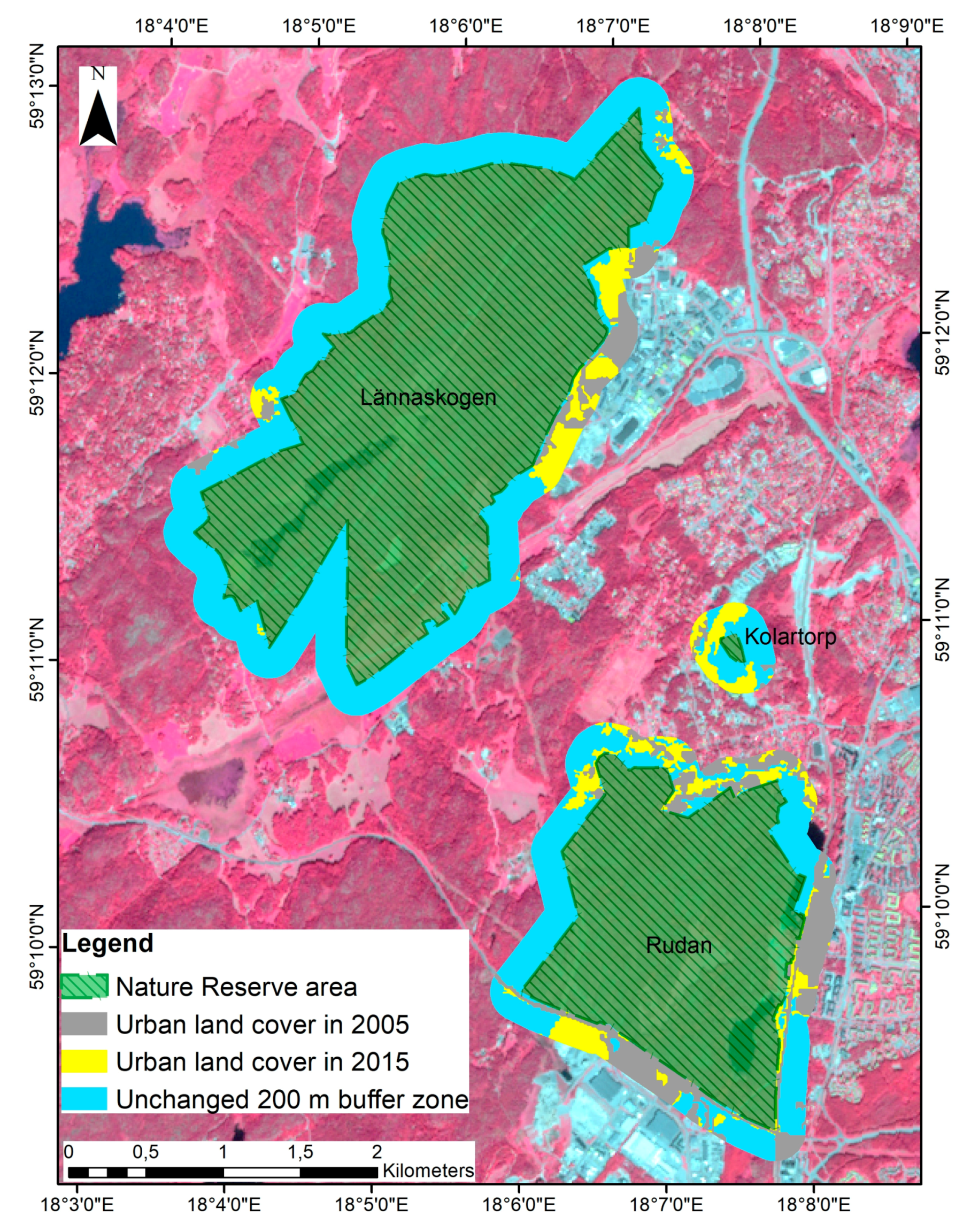
Urban Change in and around Protected and Ecologically Significant Areas

Nature Reserves
The urban area of the calculated 200 m buffer zone around the SEPA nature reserves in Stockholm County increased by 5.5 km2 between 2005 and 2015. This amounts to a 1% increase in terms of the total area of the buffer zones and a 16% increase in terms of the 2005 urban area of the zones. Graphic examples of this increase are shown in Figure 7 and Figure 8 below. Of note in Figure 8 is the expansion of urban land cover up to and along the boundary on the eastern side of the Lännaskogen Nature Reserve (NR) and to the south of Rudan NR. These expansions are both from forest to industrial/commercial land cover (HDB) and the expansion near Kolartorp is from forest to roads and residential areas (LDB).
Bornsjön NR provides another example of urban expansion up to and along its southwest boundary in Södertälje Municipality, see Figure 8. Here the southernmost expansion is from forest to industrial land cover (HDB) and the expansion to the northwest in the image is from forest to residential areas (LDB).
Some nature reserves also became increasingly surrounded by urban land cover even if this did not occur in their immediate (200 m) vicinity. Figure 9 shows how the Igelbäcken cultural and nature reserves have become more isolated from other green spaces as a result of urban expansion. In this figure, it becomes evident how Igelbäcken NR is nearly completely enclosed by urban areas. The only green link is to the east towards Ulriksdal NR.
Deciduous Ecological Corridor Network
The area of urban overlap with the deciduous ecological corridor network in Stockholm County increased by 4.6 km2 between 2005 and 2015. This amounts to a 1% increase in terms of the total network area and a 12% increase in terms of the 2005 urban area of the network. Graphic examples of overlap with the primary and secondary ecocorridors are shown in Figure 10 and Figure 11 respectively below. In these examples, forest was converted to industrial and residential land cover in Vårby and to residential land cover in Trångsund.
Green Wedges and Core Areas
The area of urban overlap with green wedges and green core areas identified in the RUFS 2050 plan for Stockholm County increased by 9.3 km2 between 2005 and 2015. This amounts to a 0.6% increase in terms of the total green wedge and core area, but an impressive 52% increase in terms of the 2005 urban overlap area. A graphic example of the urban overlap increase is shown in Figure 12 below. For core areas alone, the increase was 4.2 km2 or 0.5% increase over the total area corresponding to a 48% urban increase.
Figure 12 shows contiguous portions of three municipalities: Upplands-Bro, Upplands-Väsby and Sigtuna and urban expansion into green wedges and core areas in each. Notable areas of overlap are circled in black. Here, the land conversion was from forest and agriculture to industrial in Sigtuna, from forest to industrial in Upplands-Väsby and from forest to residential in Upplands-Bro.
The area in and around Flaten Nature Reserve in southeast Stockholm is particularly important from an ecological standpoint since all three types of green infrastructure (nature reserve, deciduous ecocorridor and green wedge core area) overlap there. Figure 13 shows the urban expansion in and around Flaten in relation to all of these. The area shown is also where the municipal boundaries of Stockholm, Nacka, Tyresö and Huddinge municipalities meet. Here is evidently an ecologically significant area under pressure from urban expansion with the added challenge of coordinating between four municipalities for decisions regarding either its preservation from or exposure to further urban development.

6. Discussion

With regard to reporting on the group of northern municipalities that experienced the most urban growth, this is partially dependent on the way administrative boundaries are drawn. More municipalities in the northern part of Stockholm County appear to be urbanizing than in the southern part, but the northern area contains a number of smaller municipalities in terms of land area compared with those to the south. This makes their urban growth appear more dramatic if only land area percentages are considered; Sundbyberg is one such example. However, Sigtuna in the north is a relatively large municipality and had the largest number of square kilometers of urban expansion (16) of any other municipality.
By contrast, the nature reserves in the northern part of the study area are relatively few and generally much smaller than those that exist south of Stockholm City. Huddinge, for example, where a number of urban expansion examples have been shown, counts no less than 11 nature reserves within its borders. The number and size of the nature reserves here place obvious constraints on where urban growth can occur and, as a result, urban expansion makes an impact on ecologically significant areas almost unavoidable.
Thus, while most urban growth occurred to the north of Stockholm City between 2005 and 2015, the most significant environmental impact registered in the south. There, the overlap with the Stockholm region’s green infrastructure was evident, as the calculations and majority of examples of urban expansion have shown. The case of Flaten Nature Reserve reveals how important ecological areas are experiencing pressure and impacts from an urban development on nearly all sides. Flaten NR also lies in the midst of three out of four important but weak regional connections for the deciduous forest ecosystem, which the green infrastructure action plan points out as in need of strengthening [74]. Flaten NR is, therefore, a key part of the ecocorridor and green wedge networks and for this reason should at least be shielded from further pressure and at most have its green linkages with other parts of the ecosystem bolstered.
Stockholm’s green infrastructure action plan notes that one of the most direct threats to forest biodiversity in the County is the loss of core areas either as a result of clear-cutting or conversion to other types of land cover [72]. One of the largest land-cover areal decreases in this study was for forested areas, where over 80 km2 were converted during the decade. Most of the examples of land conversion as a result of urban expansion presented here are of forested areas to either industrial or residential land cover. These include examples of loss of valuable green core area in Upplands-Bro municipality and loss of both primary and secondary deciduous ecocorridor forest in Huddinge municipality. These new urban areas pose problems for ecosystem function and biodiversity in the remaining nearby forest through areal loss and increased edge effects, and they strengthen the barrier effects of the existing urban areas they have been added or connected to [8,14,45,101]. These local impacts are mirrored at the regional landscape level by the negative changes in temperature regulation, noise reduction and air purification ecosystem service provision bundles, which represent fundamental ecosystem services provided by forested areas in particular. These negative changes at the landscape level were due in part to loss of forested areas but even more so to decreasing proximity of forest and increasing proximity of LDB areas, several local examples of which have been presented in regard to changes in and around specific types of green infrastructure. The reason for urban expansion in these ecologically important areas is most likely tied to their lack of formal or legislative protection combined with pressure for new urban development from an increasing population.
Yet even legally protected areas were coming under pressure from urbanization. SEPA points out that transition zones between natural and even semi-natural land cover are particularly valuable for biodiversity since they often contain species from more than one ecosystem [92]. They can also act as protective buffer zones for core ecological areas, which are often an important part of nature reserves. Investigation of change in the buffer area around legally protected nature reserves in Stockholm County revealed several examples of shrinkage and even elimination of portions of non-urban land-cover buffer areas. Urban areas built in direct proximity to important ecological or protected areas negatively impact the biodiversity and ecosystem function within through reduction of core area and edge effects such as noise and light disturbance as well as pollution. Some of the examples highlighted the problem of nature reserves becoming increasingly surrounded by urban development, even at times within their buffer zones. Such enclosure increases their isolation from other parts of the ecosystem and diminishes or eliminates green links or ecocorridors in the landscape.
Colding [22] (p. 322) states that “protected areas in Stockholm constitute a patchwork quilt of ecosystems that do not match critical ecosystem interactions and dynamics, missing the important aspects of landscape connectivity.” In that sense, urban growth impact outside of and around the protected areas gains more significance. Analysis for the identification of the deciduous ecocorridor network [75] and even the “green weak links” as first identified in the Stockholm regional development plan, RUFS 2010 [102], are efforts to highlight some of these important landscape ecological connections. Figure 14 shows the urban impact on green infrastructure examples presented earlier at a larger scale, and nearby green weak links in Stockholm’s green structure according to RUFS 2050 are shown in white [76]. Here we can see that the urban expansion (new 2015 urban areas that overlap green infrastructure are shown in yellow) is occurring in close proximity to these weak links. This is a problematic trend given the recommendations of the green infrastructure action plan and other earlier planning documentation that emphasize strengthening the green weak links [74,103]. Several weak links appear to be becoming weaker rather than stronger (e.g., south of Rudan, west of Bornsjön, in the northern part of Flaten and at several points across the Järva green wedge). Perhaps more planning focus should be shifted to the protection/restoration of affected green weak links rather than remaining on addition of new protected but often isolated patches. The findings also raise some key questions: How much of an uninterrupted buffer zone is needed to maintain the function and well-being of protected areas and how much green structure is needed to ensure the functioning of the green links and ecocorridors in the Stockholm landscape? Timely answers are needed since both have been diminished over the course of the past two decades.
Nature reserves in Sweden are established on a case by case basis usually initiated by a proposal from county authorities. It is therefore worth noting that nature reserves in Stockholm County date from different years. Of the reserves mentioned in this study, Bornsjön is likely the oldest as it was established in 1995, followed by Lännaskogen established in 2002 and Igelbäcken established in 2004, just before the beginning of the study period. Flaten, Rudan and Kolartorp are newer reserves, however, established in 2007, 2010 and 2011 respectively. One might wonder if these reserves were established in response to urban growth and pressure occurring in their vicinity. This may have been true for Rudan where inspection of Google Earth historical images reveals that conversion of the buffer area to the south began in 2008, two years before it became a nature reserve, and continued into 2012. Yet the urban growth to the west of Flaten occurred in early 2015 and the clear-cutting of forest that occurred in its northern section between the roads that traverse it occurred somewhere between 2008 and 2010, well after the nature reserve was established. The urban expansion surrounding Kolartorp began somewhere between 2012 and 2014, after its establishment as a reserve in 2011. So the establishment of a nature reserve appears to have little influence one way or another on conversion of land cover in its immediate vicinity. Borgström et al. [104] found that the establishment of nature reserves had no detectable effect on surrounding land use from their analysis of change in buffer zones around nature reserves in southern Sweden.
There was a small (<1%) overall loss in ecosystem service value where the increase in UGS compensated to a significant degree the decrease in forest and proximate green/blue structure. Yet given Stockholm’s plans for continued substantial urban expansion [76], is this amount of decadal ecosystem service loss acceptable and sustainable in the long run? It is worth noting that the monetary value for urban greenspace is roughly twice as much as for forest. While the valuation scheme adapted and used here is largely suited to Stockholm, where forest is relatively plentiful and where semi-open landscape and grasslands have a long tradition and value from Swedish agro-pastoral history [105], it may not be appropriate in other regions where, for example, forest may be scarce and/or desertification or erosion may be a problem. The determination of monetary value for ecosystem service providing land cover plays a significant role in the ecosystem service balance results obtained and should where possible be regionally adapted.
The landscape metric-based ecosystem service provision bundles proposed by Haas and Ban [21] and here adapted and tested with higher resolution Sentinel-2 and SPOT-5 data were able to register the more subtle impacts on ecosystem service provision in Stockholm County. While environmental impact in more rapidly urbanizing areas can often be clearly detected with various indicators, this is not always the case for regions with a significant proportion of green area urbanizing at a more moderate pace such as Stockholm’s, e.g., [65].
A positive finding for ecosystem service provision in the Stockholm region is that wetlands remained more or less stable in terms of the area during this time period and did not register significant impact from urban growth. However, 10 m resolution may not be fine enough for examination of wetlands in this geographic region since they are often much smaller in size than, for example, forested areas. Assessment of their status through a higher resolution change study might reveal more subtle urban growth impacts or pressure that are not possible to detect with this data and methodology.

Limitations and Transferability of the Applied Methodology

The methodology for this study has been developed with a landscape regional level in mind, which often involves study areas of several thousands of square kilometers. Appropriate data in the form Sentinel-2 and SPOT imagery proves useful for such an undertaking given the wide coverage paired with enough detail to evaluate significant change. However, uncertainty is an intrinsic part of remote sensing of the environment in that the data is collected from a distance. Given the study area size and geophysical variation, the resolution of the satellite imagery, and high-performing although imperfect classifier algorithms, the classification results are limited by a certain amount of error, and this error will have a tendency to propagate as indicators are calculated. Evaluating the accuracy allows investigators to decide if the classification results are accurate enough for analysis and indicator calculation, which was the case in this study.
For this investigation, accuracy was evaluated at the landscape regional level and thus conclusions about general trends in the landscape, i.e., green structure and ecosystem service change, will be most reliable, while results on more localized levels, i.e., municipalities and nature reserves, will be less certain. This motivated the choice to aggregate the urban and green structure classes prior to calculating indicators on these levels, in order to increase their reliability and lower the effects of error propagation.
The employed method of evaluation of ecosystem service change relies on the composition and spatial configuration of land cover. It does not measure specific biophysical changes in ecosystem health or service provision within Stockholm’s green infrastructure. Therefore, process models based on empirical data applied in this region could be a useful complement in monitoring ecosystem function or service change.
The urbanization of Stockholm is occurring at a relatively moderate pace if one compares with other major cities of similar geographic extent. The methodology applied here should, therefore, be adequate to detect change in a majority of other locations. But transferring this study’s methodology in order to monitor progress towards SDG 15 would require a number of regional adaptations. A tailored classification scheme should be selected as well as relevant ancillary data if available for classification improvement. The SVM algorithm was employed in this study but it is possible that other high-performance classifiers such as random forest may work better in other contexts (e.g., considering the characteristics of the imagery, classification scheme and/or computing capacity available). Some of the spatial attribute ecological principles listed in Section 4.3.1 are widely applicable (e.g., area) while others are dependent on the context of the landscape matrix they are applied to (e.g., diversity). Ideally, local conservation or planning authorities might provide ecological criteria that could serve as a basis for landscape metric selection and ecosystem service bundle construction. The importance of a locally appropriate valuation scheme has already been mentioned. The possibility to examine urban impact on regional green infrastructure will depend on the availability of site-specific green infrastructure datasets such as nature reserve/valuable biotope maps or ecological corridor analyses. If these are lacking, then this could highlight the need for their development in support of planning for sustainable urban development.
The results of this study are constrained by the Stockholm County boundary, which does not represent green infrastructure boundaries and thus cannot provide information regarding transboundary environmental changes/issues on the outskirts of the study area. The county boundary was used nonetheless since the majority of urban growth occurred in the more central parts of the county and not in proximity to its boundaries and since planning authorities often require statistics according to administrative boundaries for various purposes. The deciduous ecocorridor study obtained results regarding this type of green infrastructure’s status across county lines [75]. Future studies analyzing green structure on the outskirts of the county would require different and more ecologically appropriate study area dimensions.

7. Conclusions

This research investigates urban expansion in Stockholm County between 2005 and 2015 and the resulting environmental impact based on object-oriented SVM classifications of Sentinel-2A MSI and SPOT-5 HRI data. Similar high accuracies (kappa: 0.88) were achieved for both classifications, but Sentinel-2A MSI data proved particularly useful in its coverage of nearly the entire study area by one image and its variety of spectral bands which contributed to better classification of agriculture, forest and wetland classes when compared to the classification of the SPOT-5 HRI data. The landscape metric-based urban ecosystem service bundles proposed by Haas and Ban proved effective in capturing changes in service provision in Stockholm’s moderately urbanizing landscape based on the object-based SVM classifications of higher resolution Sentinel-2A and SPOT-5 data. In addition to calculation of urban growth statistics on administrative levels, this study also highlights localized urban growth impacts on legally protected nature reserves and the region’s ecogically significant green infrastructure, the management of which in some cases is the responsibility of more than one municipality.
Urban areas increased by approximately 15% while non-urban land-cover types decreased by about 4% or 116 km2. The results suggest that urban areas may soon overtake agricultural areas to become the second-largest land-cover category in the county landscape after forest. Forest was the vegetated land-cover category most impacted by urban growth over the decade, with a total loss of over 80 km2. This contributed to impacts on ecosystem service provision, with small but notable decreases in food supply, waste treatment and global climate regulation. However, decrease in proximity of forest and increase in proximity of LDB areas were the main cause of greater decreases in temperature regulation, air purification and noise reduction as well as recreation, place values and social cohesion. Ecosystem service loss over the decade amounted to 4.6 million USD (2015 exchange rate).
The largest increases in urban areas and significant losses of green structure occurred mainly in the northern area of the county in the rural-urban fringe. However, the most significant environmental impact registered south of Stockholm City where urban expansion increasingly overlapped several types of the region’s protected and ecologically important green infrastructure. Urban areas within a 200 m buffer zone around the SEPA nature reserves in Stockholm County increased by 16% over the decade, with several examples of new urban areas constructed along the boundary of nature reserves. Urban expansion also overlapped the deciduous ecological corridor network and green wedge and core areas to a relatively small but increasing degree. Comparison of urban growth with weak links in Stockholm’s green infrastructure revealed that certain ecologically important connections in the landscape may be getting weaker in spite of calls to strengthen them. Given these findings, increased conservation/restoration focus on the region’s green weak links is recommended. A continually updated spatio-temporal analysis of key ecological areas and buffer zones, and their comparison with existing weak green links, could be a helpful part of future environmental monitoring so that planning resources and restorative efforts are targeted to the right places in a timely manner. Given the effectiveness of the combined data and methodology in monitoring urban change and environmental impact in a moderately urbanizing region such as Stockholm, the application of similar techniques adapted to the local environmental context in other urbanizing regions could prove useful in evaluating progress toward national and international sustainability goals.

Author Contributions

Conceptualization, Y.B. and D.F.; methodology, D.F., Y.B. and A.N.; validation, D.F.; formal analysis, D.F.; investigation, D.F.; resources, Y.B.; data curation, D.F.; writing—original draft preparation, D.F.; writing—review and editing, Y.B. and A.N.; visualization, D.F.; supervision, Y.B. and A.N.; project administration, Y.B.; funding acquisition, Y.B.

Funding

This research was funded by the Swedish National Space Agency, grant number dnr 155/15.

Acknowledgments

The authors especially thank Jan Haas for discussions and information regarding ecosystem service bundle construction. They are also grateful to Saccess for providing access to the SPOT-5 data, to the European Space Agency for the Sentinel-2A MSI data and to the Stockholm County Administrative Board for providing the nature reserve and deciduous ecocorridor geographic datasets.

Conflicts of Interest

The authors declare no conflict of interest.

References

  1. United Nations. World Urbanization Prospects: The 2018 Revision, Key Facts. Department of Economic and Social Affairs, Population Division, 2018. Available online: https://population.un.org/wup/Publications/Files/WUP2018-KeyFacts.pdf (accessed on 21 April 2019).
  2. Grimm, N.B.; Faeth, S.H.; Golubiewski, N.E.; Redman, C.L.; Wu, J.; Bai, X.; Briggs, J.M.; Grimm, N. Global Change and the Ecology of Cities. Science 2008, 319, 756–760. [Google Scholar] [CrossRef] [PubMed] [Green Version]
  3. Seto, K.C.; Fragkias, M.; Güneralp, B.; Reilly, M.K. A Meta-Analysis of Global Urban Land Expansion. PLoS ONE 2011, 6, e23777. [Google Scholar] [CrossRef] [PubMed]
  4. Alberti, M. Advances in Urban Ecology: Integrating Humans and Ecological Processes in Urban Ecosystems (No. 574.5268 A4); Springer: New York, NY, USA, 2008; p. 366. [Google Scholar] [CrossRef]
  5. Heilman, G.E.; Strittholt, J.R.; Slosser, N.C.; Dellasala, D.A. Forest Fragmentation of the Conterminous United States: Assessing Forest Intactness through Road Density and Spatial Characteristics: Forest fragmentation can be measured and monitored in a powerful new way by combining remote sensing, geographic information systems, and analytical software. BioScience 2002, 52, 411–422. [Google Scholar]
  6. Imhoff, M.L.; Zhang, P.; Wolfe, R.E.; Bounoua, L. Remote sensing of the urban heat island effect across biomes in the continental USA. Remote Sens. Environ. 2010, 114, 504–513. [Google Scholar] [CrossRef] [Green Version]
  7. Williams, N.S.; Schwartz, M.W.; Vesk, P.A.; McCarthy, M.A.; Hahs, A.K.; Clemants, S.E.; Corlett, R.T.; Duncan, R.P.; Norton, B.A.; Thompson, K.; et al. A conceptual framework for predicting the effects of urban environments on floras. J. Ecol. 2009, 97, 4–9. [Google Scholar] [CrossRef]
  8. Lindenmayer, D.B.; Fischer, J. Habitat Fragmentation and Landscape Change: An Ecological and Conservation Synthesis; Island Press: Washington, DC, USA, 2006; ISBN 1-59726-021-5. [Google Scholar]
  9. Turner, M.G. Landscape Ecology: The Effect of Pattern on Process. Annu. Rev. Ecol. Syst. 1989, 20, 171–197. [Google Scholar] [CrossRef]
  10. Hasse, J.E.; Lathrop, R.G. Land resource impact indicators of urban sprawl. Appl. Geogr. 2003, 23, 159–175. [Google Scholar] [CrossRef]
  11. Pickett, S.T.; Cadenasso, M.L. Altered resources, disturbance, and heterogeneity: A framework for comparing urban and non-urban soils. Urban Ecosyst. 2009, 12, 23–44. [Google Scholar] [CrossRef]
  12. O’Driscoll, M.; Clinton, S.; Jefferson, A.; Manda, A.; McMillan, S. Urbanization Effects on Watershed Hydrology and In-Stream Processes in the Southern United States. Water 2010, 2, 605–648. [Google Scholar] [CrossRef]
  13. Stutzer, D.; Lawrence, W.; Tucker, C.; Imhoff, M. The use of multisource satellite and geospatial data to study the effect of urbanization on primary productivity in the United States. IEEE Trans. Geosci. Remote Sens. 2000, 38, 2549–2556. [Google Scholar] [CrossRef] [Green Version]
  14. Hilty, J.A.; Lidicker, W.Z., Jr.; Merenlender, A.M. Corridor Ecology: The Science and Practice of Linking Landscapes for Biodiversity Conservation; Island Press: Washington, DC, USA, 2012; ISBN 1-55963-096-5. [Google Scholar]
  15. Sustainable Development Goal 15. Available online: https://sustainabledevelopment.un.org/sdg15 (accessed on 6 August 2019).
  16. UN-DESA Division for Sustainable Development Goals. Sustainable Development Goal 15: Progress and Prospects, Outcome: Key Messages. In Proceedings of the An Expert Group Meeting in Preparation for HLPF 2018: Transformation Towards Sustianable and Resilient Societies, New York, NY, USA, 14–15 May 2018; Available online: https://sustainabledevelopment.un.org/content/documents/19647Key_messages_SDG_15_EGM_Final.pdf (accessed on 21 April 2019).
  17. Weng, Q.; Quattrochi, D.; Gamba, P.E. Urban Remote Sensing, 2nd ed.; CRC press, Taylor & Francis Group: Boca Raton, FL, USA, 2018. [Google Scholar] [CrossRef]
  18. Ban, Y.; Gong, P.; Giri, C. Global land cover mapping using Earth observation satellite data: Recent progresses and challenges. ISPRS J. Photogramm. Remote Sens. 2015, 103, 1–6. [Google Scholar] [CrossRef] [Green Version]
  19. Pesaresi, M.; Corbane, C.; Julea, A.; Florczyk, A.J.; Syrris, V.; Soille, P. Assessment of the Added-Value of Sentinel-2 for Detecting Built-up Areas. Remote Sens. 2016, 8, 299. [Google Scholar] [CrossRef]
  20. Deng, J.; Huang, Y.; Chen, B.; Tong, C.; Liu, P.; Wang, H.; Hong, Y. A Methodology to Monitor Urban Expansion and Green Space Change Using a Time Series ofMulti-Sensor SPOT and Sentinel-2A Images. Remote Sens. 2019, 11, 1230. [Google Scholar] [CrossRef]
  21. Haas, J.; Ban, Y. Urban Land Cover and Ecosystem Service Changes based on Sentinel-2A MSI and Landsat TM Data. IEEE J. Sel. Top. Appl. Earth Obs. Remote Sens. 2018, 11, 485–497. [Google Scholar] [CrossRef]
  22. Colding, J. Local Assessment of Stockholm: Revisiting the Stockholm Urban Assessment. In Urbanization, Biodiversity and Ecosystem Services: Challenges and Opportunities: A Global Assessment; Elmqvist, T., Fragkias, M., Goodness, J., Güneralp, B., Marcotullio, P.J., McDonald, R.I., Parnell, S., Schewenius, M., Sendstad, M., Seto, K.C., et al., Eds.; Springer: Dordrecht, Germany, 2013; pp. 313–335. [Google Scholar] [CrossRef] [Green Version]
  23. Herold, M.; Couclelis, H.; Clarke, K.C. The role of spatial metrics in the analysis and modeling of urban land use change. Comput. Environ. Urban Syst. 2005, 29, 369–399. [Google Scholar] [CrossRef]
  24. Ma, L.; Li, M.; Ma, X.; Cheng, L.; Du, P.; Liu, Y. A review of supervised object-based land-cover image classification. ISPRS J. Photogramm. Remote Sens. 2017, 130, 277–293. [Google Scholar] [CrossRef]
  25. Myint, S.W.; Gober, P.; Brazel, A.; Grossman-Clarke, S.; Weng, Q. Per-pixel vs. object-based classification of urban land cover extraction using high spatial resolution imagery. Remote Sens. Environ. 2011, 115, 1145–1161. [Google Scholar] [CrossRef]
  26. Ban, Y.; Hu, H.; Rangel, I.M. Fusion of Quickbird MS and RADARSAT SAR data for urban land-cover mapping: Object-based and knowledge-based approach. Int. J. Remote Sens. 2010, 31, 1391–1410. [Google Scholar] [CrossRef]
  27. Wentz, E.A.; Anderson, S.; Fragkias, M.; Netzband, M.; Mesev, V.; Myint, S.W.; Quattrochi, D.; Rahman, A.; Seto, K.C. Supporting Global Environmental Change Research: A Review of Trends and Knowledge Gaps in Urban Remote Sensing. Remote Sens. 2014, 6, 3879–3905. [Google Scholar] [CrossRef] [Green Version]
  28. Patino, J.E.; Duque, J.C. A review of regional science applications of satellite remote sensing in urban settings. Comput. Environ. Urban Syst. 2013, 37, 1–17. [Google Scholar] [CrossRef]
  29. Jacquin, A.; Misakova, L.; Gay, M. A hybrid object-based classification approach for mapping urban sprawl in periurban environment. Landsc. Urban Plan. 2008, 84, 152–165. [Google Scholar] [CrossRef]
  30. Lu, D.; Weng, Q. Urban classification using full spectral information of Landsat ETM+ imagery in Marion County, Indiana. Photogramm. Eng. Remote Sens. 2005, 71, 1275–1284. [Google Scholar] [CrossRef]
  31. Phiri, D.; Morgenroth, J. Developments in Landsat Land Cover Classification Methods: A Review. Remote Sens. 2017, 9, 967. [Google Scholar] [CrossRef]
  32. Powers, R.P.; Hay, G.J.; Chen, G. How wetland type and area differ through scale: A GEOBIA case study in Alberta’s Boreal Plains. Remote Sens. Environ. 2012, 117, 135–145. [Google Scholar] [CrossRef]
  33. Jebur, M.N.; Mohd Shafri, H.Z.; Pradhan, B.; Tehrany, M.S. Per-pixel and object-oriented classification methods for mapping urban land cover extraction using SPOT 5 imagery. Geocarto Int. 2014, 29, 792–806. [Google Scholar] [CrossRef]
  34. Tehrany, M.S.; Pradhan, B.; Jebuv, M.N. A comparative assessment between object and pixel-based classification approaches for land use/land cover mapping using SPOT 5 imagery. Geocarto Int. 2014, 29, 351–369. [Google Scholar] [CrossRef]
  35. Chen, M.; Su, W.; Li, L.; Zhang, C.; Yue, A.; Li, H. Comparison of pixel-based and object-oriented knowledge-based classification methods using SPOT5 imagery. WSEAS Trans. Inf. Sci. Appl. 2009, 3, 477–489. [Google Scholar]
  36. Lu, D.; Weng, Q. A survey of image classification methods and techniques for improving classification performance. Int. J. Remote Sens. 2007, 28, 823–870. [Google Scholar] [CrossRef]
  37. Ghosh, A.; Joshi, P. A comparison of selected classification algorithms for mapping bamboo patches in lower Gangetic plains using very high resolution WorldView 2 imagery. Int. J. Appl. Earth Obs. Geoinf. 2014, 26, 298–311. [Google Scholar] [CrossRef]
  38. Guan, H.; Li, J.; Chapman, M.; Deng, F.; Ji, Z.; Yang, X. Integration of orthoimagery and lidar data for object-based urban thematic mapping using random forests. Int. J. Remote Sens. 2013, 34, 5166–5186. [Google Scholar] [CrossRef]
  39. Niu, X.; Ban, Y. Multi-temporal RADARSAT-2 polarimetric SAR data for urban land-cover classification using an object-based support vector machine and a rule-based approach. Int. J. Remote Sens. 2013, 34, 1–26. [Google Scholar] [CrossRef]
  40. Huang, C.; Davis, L.S.; Townshend, J.R.G. An assessment of support vector machines for land cover classification. Int. J. Remote Sens. 2002, 23, 725–749. [Google Scholar] [CrossRef]
  41. Tzotsos, A.; Argialas, D. Support Vector Machine Classification for Object-Based Image Analysis. In Lecture Notes in Geoinformation and Cartography; Springer Science and Business Media LLC: Berlin, Germany, 2008; pp. 663–677. [Google Scholar]
  42. Momeni, R.; Aplin, P.; Boyd, D.S. Mapping Complex Urban Land Cover from Spaceborne Imagery: The Influence of Spatial Resolution, Spectral Band Set and Classification Approach. Remote Sens. 2016, 8, 88. [Google Scholar] [CrossRef]
  43. Thanh Noi, P.; Kappas, M. Comparison of random forest, k-nearest neighbor, and support vector machine classifiers for land cover classification using Sentinel-2 imagery. Sensors 2018, 18, 18. [Google Scholar] [CrossRef]
  44. Millennium Ecosystem Assessment. Ecosystems and Human Well-Being: Synthesis; Island Press: Washington, DC, USA, 2005. [Google Scholar]
  45. Haddad, N.M.; Brudvig, L.A.; Clobert, J.; Davies, K.F.; Gonzalez, A.; Holt, R.D.; Lovejoy, T.E.; Sexton, J.O.; Austin, M.P.; Collins, C.D.; et al. Habitat fragmentation and its lasting impact on Earth’s ecosystems. Sci. Adv. 2015, 1, e1500052. [Google Scholar] [CrossRef]
  46. Newbold, T.; Hudson, L.N.; Hill, S.L.L.; Contu, S.; Lysenko, I.; Senior, R.A.; Borger, L.; Bennett, D.J.; Choimes, A.; Collen, B.; et al. Global effects of land use on local terrestrial biodiversity. Nature 2015, 520, 45–50. [Google Scholar] [CrossRef] [PubMed] [Green Version]
  47. Seto, K.C.; Güneralp, B.; Hutyra, L.R. Global forecasts of urban expansion to 2030 and direct impacts on biodiversity and carbon pools. Proc. Natl. Acad. Sci. USA 2012, 109, 16083–16088. [Google Scholar] [CrossRef] [Green Version]
  48. Alberti, M. The Effects of Urban Patterns on Ecosystem Function. Int. Reg. Sci. Rev. 2005, 28, 168–192. [Google Scholar] [CrossRef]
  49. Haas, J.; Ban, Y. Urban growth and environmental impacts in Jing-Jin-Ji, the Yangtze, River Delta and the Pearl River Delta. Int. J. Appl. Earth Obs. Geoinf. 2014, 30, 42–55. [Google Scholar] [CrossRef]
  50. Andrew, M.E.; Wulder, M.A.; Nelson, T.A.; Coops, N.C. Spatial data, analysis approaches, and information needs for spatial ecosystem service assessments: A review. GIScience Remote Sens. 2015, 52, 344–373. [Google Scholar] [CrossRef]
  51. Barbosa, C.C.D.A.; Atkinson, P.M.; Dearing, J.A. Remote sensing of ecosystem services: A systematic review. Ecol. Indic. 2015, 52, 430–443. [Google Scholar] [CrossRef]
  52. Ayanu, Y.Z.; Conrad, C.; Nauss, T.; Wegmann, M.; Koellner, T. Quantifying and Mapping Ecosystem Services Supplies and Demands: A Review of Remote Sensing Applications. Environ. Sci. Technol. 2012, 46, 8529–8541. [Google Scholar] [CrossRef] [PubMed]
  53. De La Barrera, F.; Rubio, P.; Banzhaf, E. The value of vegetation cover for ecosystem services in the suburban context. Urban For. Urban Green. 2016, 16, 110–122. [Google Scholar] [CrossRef]
  54. Gómez-Baggethun, E.; Gren, Å.; Barton, D.N.; Langemeyer, J.; McPhearson, T.; O’Farrell, P.; Andersson, E.; Hamstead, Z.; Kremer, P. Urban Ecosystem Services. In Urbanization, Biodiversity and Ecosystem Services: Challenges and Opportunities: A Global Assessment; Elmqvist, T., Fragkias, M., Goodness, J., Güneralp, B., Marcotullio, P.J., McDonald, R.I., Parnell, S., Schewenius, M., Sendstad, M., Seto, K.C., et al., Eds.; Springer: Dordrecht, Germany, 2013; pp. 175–251. [Google Scholar] [CrossRef]
  55. Bolund, P.; Hunhammar, S. Ecosystem services in urban areas. Ecol. Econ. 1999, 29, 293–301. [Google Scholar] [CrossRef]
  56. Frank, S.; Fürst, C.; Koschke, L.; Makeschin, F. A contribution towards a transfer of the ecosystem service concept to landscape planning using landscape metrics. Ecol. Indic. 2012, 21, 30–38. [Google Scholar] [CrossRef]
  57. Duarte, G.T.; Santos, P.M.; Cornelissen, T.G.; Ribeiro, M.C.; Paglia, A.P. The effects of landscape patterns on ecosystem services: Meta-analyses of landscape services. Landsc. Ecol. 2018, 33, 1247–1257. [Google Scholar] [CrossRef]
  58. Bagstad, K.J.; Johnson, G.W.; Voigt, B.; Villa, F. Spatial dynamics of ecosystem service flows: A comprehensive approach to quantifying actual services. Ecosyst. Serv. 2013, 4, 117–125. [Google Scholar] [CrossRef]
  59. Syrbe, R.-U.; Walz, U. Spatial indicators for the assessment of ecosystem services: Providing, benefiting and connecting areas and landscape metrics. Ecol. Indic. 2012, 21, 80–88. [Google Scholar] [CrossRef]
  60. Uuemaa, E.; Antrop, M.; Roosaare, J.; Marja, R.; Mander, U. Landscape Metrics and Indices: An Overview of Their Use in Landscape Research. Living Rev. Landsc. Res. 2009, 3, 1–28. [Google Scholar] [CrossRef]
  61. Uuemaa, E.; Mander, U.; Marja, R. Trends in the use of landscape spatial metrics as landscape indicators: A review. Ecol. Indic. 2013, 28, 100–106. [Google Scholar] [CrossRef]
  62. Leitão, A.B.; Ahern, J. Applying landscape ecological concepts and metrics in sustainable landscape planning. Landsc. Urban Plan. 2002, 59, 65–93. [Google Scholar] [CrossRef]
  63. Turner, M.G. Spatial and temporal analysis of landscape patterns. Landsc. Ecol. 1990, 4, 21–30. [Google Scholar] [CrossRef]
  64. Gbanie, S.P.; Griffin, A.L.; Thornton, A. Impacts on the Urban Environment: Land Cover Change Trajectories and Landscape Fragmentation in Post-War Western Area, Sierra Leone. Remote Sens. 2018, 10, 129. [Google Scholar] [CrossRef]
  65. Haas, J.; Furberg, D.; Ban, Y. Satellite monitoring of urbanization and environmental impacts—A comparison of Stockholm and Shanghai. Int. J. Appl. Earth Obs. Geoinf. 2015, 38, 138–149. [Google Scholar] [CrossRef]
  66. Furberg, D.; Ban, Y. Satellite Monitoring of Urban Sprawl and Assessment of its Potential Environmental Impact in the Greater Toronto Area Between 1985 and 2005. Environ. Manag. 2012, 50, 1068–1088. [Google Scholar] [CrossRef]
  67. Su, S.; Xiao, R.; Jiang, Z.; Zhang, Y. Characterizing landscape pattern and ecosystem service value changes for urbanization impacts at an eco-regional scale. Appl. Geogr. 2012, 34, 295–305. [Google Scholar] [CrossRef]
  68. Lausch, A.; Blaschke, T.; Haase, D.; Herzog, F.; Syrbe, R.-U.; Tischendorf, L.; Walz, U. Understanding and quantifying landscape structure—A review on relevant process characteristics, data models and landscape metrics. Ecol. Model. 2015, 295, 31–41. [Google Scholar] [CrossRef]
  69. Turner, M.G.; Donato, D.C.; Romme, W.H. Consequences of spatial heterogeneity for ecosystem services in changing forest landscapes: Priorities for future research. Landsc. Ecol. 2013, 28, 1081–1097. [Google Scholar] [CrossRef]
  70. Burkhard, B.; Petrosillo, I.; Costanza, R. Ecosystem services—Bridging ecology, economy and social sciences. Ecol. Complex. 2010, 7, 257–259. [Google Scholar] [CrossRef]
  71. Maltby, E.; Acreman, M.C. Ecosystem services of wetlands: Pathfinder for a new paradigm. Hydrol. Sci. J. 2011, 56, 1341–1359. [Google Scholar] [CrossRef]
  72. Colding, J.; Elmqvist, T.; Lundberg, J.; Ahrné, K.; Andersson, E.; Barthel, S.; Borgström, S.; Duit, A.; Ernstsson, H.; Tengö, M. The Stockholm Urban Assessment (SUA-Sweden). In Millennium Ecosystem Assessment Sub-Global Summary Report; Beijer Discussion Paper Series No. 182; The Beijer Institute of Ecological Economics, Royal Academy of Sciences: Stockholm, Sweden, 2003; p. 28. [Google Scholar]
  73. Borgström, S. Management of Urban Green Areas in the Stockholm County. Master’s Thesis, Department of Systems Ecology, Stockholm University, Stockholm, Sweden, 2003. [Google Scholar]
  74. Länsstyrelsen Stockholm [Stockholm County Administrative Board]. Förslag Till Grön Infrastruktur Regional Handlingsplan för Stockholms Län [Draft—Green Infrastructure: Regional Action Plan for Stockholm County]. Report 2018:1. Version 2018-02-15; ISBN 978-91-7281-788-3. Available online: https://www.lansstyrelsen.se/download/18.276e13411636c95dd933a55/1526903019168/Rapport%202018-1%20F%C3%B6rslag%20till%20gr%C3%B6n%20infrastruktur%20regional%20handlingsplan%20f%C3%B6r%20Stockholms%20l%C3%A4n.pdf (accessed on 21 April 2019). (In Swedish)
  75. Ekologigruppen AB. Regional Grön Infrastruktur i Stockholms Län: Bakgrund för Analyser av Värdekärnor och Spridningszoner [Regional Green Infrastructure in Stockholm County: Background for the Analysis of Core Areas and Ecological Zones]. Information about the Project. Copies of the Report Can Be Obtained from the Stockholm County Administrative Board. 2017. Available online: https://www.ekologigruppen.se/projekt/gron-infrastruktur-stockholms-lan/ (accessed on 21 April 2019). (In Swedish).
  76. Tillväxt- och Regionplaneförvaltningen (TRF). Regional Utvecklingsplan för Stockholmsregionen: RUFS 2050 [Regional Development Plan for the Stockholm Region 2050]. Report 2018:10. TRN 2015-0015. Available online: http://rufs.se/globalassets/e.-rufs-2050/rufs_regional_utvecklingsplan_for_stockholmsregionen_2050_tillganglig.pdf (accessed on 21 April 2019). (In Swedish).
  77. Stockholmsstad. Statististical Year-Book of Stockholm 2018; Stockholm City: Stockholm, Sweden, 2018; ISBN 91-89311-01-9. Available online: http://statistik.stockholm.se/attachments/article/38/Statistisk%20%C3%83%C2%A5rsbok%20f%C3%83%C2%B6r%20Stockholm%202018.pdf (accessed on 21 April 2019).
  78. Metzger, J.; Olsson, A.R. Sustainable Stockholm: Exploring Urban Sustainability in Europe’s Greenest City; Routledge: New York, NY, USA, 2013. [Google Scholar] [CrossRef]
  79. Nelson, A. Stockholm Case Study: City of Water. In Open Space Systems Report; University of Washington: Washington, DC, USA, 2006; Available online: https://depts.washington.edu/open2100/Resources/1_OpenSpaceSystems/Open_Space_Systems/Stockholm_Case_Study.pdf (accessed on 21 April 2019).
  80. Zhang, Y. Problems in the fusion of commercial high-resolution satellite as well as Landsat 7 images and initial solutions. Int. Arch. Photogramm. Remote Sens. Spat. Inf. Sci. 2002, 34, 587–592. [Google Scholar]
  81. Lin, C.; Wu, C.-C.; Tsogt, K.; Ouyang, Y.-C.; Chang, C.-I. Effects of atmospheric correction and pansharpening on LULC classification accuracy using WorldView-2 imagery. Inf. Process. Agric. 2015, 2, 25–36. [Google Scholar] [CrossRef] [Green Version]
  82. European Space Agency. Sentinel-2 User Handbook. ESA Standard Document, 24/07/2015 Issue 1 Rev 2. 2015. Available online: https://sentinel.esa.int/documents/247904/685211/Sentinel-2_User_Handbook (accessed on 21 April 2019).
  83. Lantmäteriet [Swedish National Land Survey]. Product Description: GSD-Elevation Data, Grid 50+ nh. Document Version 1.2, 25/02/2019. Available online: https://www.lantmateriet.se/globalassets/kartor-och-geografisk-information/hojddata/e_grid50_plus_nh.pdf (accessed on 21 April 2019).
  84. Trimble Germany GmbH. eCognition Developer 9.2 Reference Book; Document Version 9.2.1; Trimble Germany GmbH: Munich, Germany, 2016. [Google Scholar]
  85. Shaban, M.A.; Dikshit, O. Improvement of classification in urban areas by the use of textural features: The case study of Lucknow city, Uttar Pradesh. Int. J. Remote Sens. 2001, 22, 565–593. [Google Scholar] [CrossRef]
  86. De Martinao, M.; Causa, F.; Serpico, S.B. Classification of optical high resolution images in urban environment using spectral and textural information. In IGARSS 2003, Proceedings of the 2003 IEEE International Geoscience and Remote Sensing Symposium, Toulouse, France, 21–25 July 2003; IEEE: Piscataway, NJ, USA, 2003; Volume 1, pp. 467–469. [Google Scholar] [CrossRef]
  87. Su, W.; Li, J.; Chen, Y.; Liu, Z.; Zhang, J.; Low, T.M.; Suppiah, I.; Hashim, S.A.M. Textural and local spatial statistics for the object-oriented classification of urban areas using high resolution imagery. Int. J. Remote Sens. 2008, 29, 3105–3117. [Google Scholar] [CrossRef]
  88. Statistics Sweden. Tätorter Referensår 2010 [Population Centers Reference Year 2010]; Avdelningen för Regioner Och Miljö, SCB: Stockholm, Sweden, 2017. Available online: http://www.scb.se/hitta-statistik/regional-statistik-och-kartor/geodata/oppna-geodata/tatorter/ (accessed on 22 April 2019).
  89. Hsu, F.-C.; Baugh, K.E.; Ghosh, T.; Zhizhin, M.; Elvidge, C.D. DMSP-OLS Radiance Calibrated Nighttime Lights Time Series with Intercalibration. Remote Sens. 2015, 7, 1855–1876. [Google Scholar] [CrossRef] [Green Version]
  90. McGarigal, K.; Cushman, S.A.; Ene, E. FRAGSTATS v4: Spatial Pattern Analysis Program for Categorical and Continuous Maps. Computer Software Program Produced by the Authors at the University of Massachusetts, Amerst, MA, USA. 2012. Available online: https://www.umass.edu/landeco/research/fragstats/fragstats.html (accessed on 22 April 2019).
  91. Liu, S.; Costanza, R.; Troy, A.; D’Aagostino, J.; Mates, W. Valuing New Jersey’s Ecosystem Services and Natural Capital: A Spatially Explicit Benefit Transfer Approach. Environ. Manag. 2010, 45, 1271–1285. [Google Scholar] [CrossRef] [PubMed]
  92. Naturvårdsverket [Swedish Environmental Protection Agency]. Riktlinjer för Regionala Handlingsplaner för Grön Infrastruktur [Guidelines for Regional Action Plans for Green Infrastructure]; Naturvårdsverket: Stockholm, Sweden, 2015; ISBN 978-91-620-0000-0. Available online: http://www.naturvardsverket.se/upload/miljoarbete-i-samhallet/miljoarbete-i-sverige/regeringsuppdrag/2015/ru-gron-infrastruktur-delredovisning/ru-gron-infrastruktur-riktlinjer-20150924.pdf (accessed on 22 April 2019). (In Swedish)
  93. Att Bilda Naturreservat [To Establish a Nature Reserve]. Available online: https://www.naturvardsverket.se/Miljoarbete-i-samhallet/Miljoarbete-i-Sverige/Uppdelat-efter-omrade/Naturvard/Skydd-av-natur/Naturreservat/ (accessed on 6 August 2019). (In Swedish).
  94. Gascon, C. ECOLOGY: Receding Forest Edges and Vanishing Reserves. Science 2000, 288, 1356–1358. [Google Scholar] [CrossRef]
  95. Murcia, C. Edge effects in fragmented forests: Implications for conservation. Trends Ecol. Evol. 1995, 10, 58–62. [Google Scholar] [CrossRef]
  96. Olsén, S.R. Arealkrav og Behov for Buffersoner ved Vern av Urørt Barskog. [Area Requirements and Need for Buffer Zones in Protection of Coniferous Forest]. Ph.D. Thesis, Norwegian Forest Research Institute, Ås, Norway, 1988. (In Norwegian, with English summary). [Google Scholar]
  97. Thorell, M.; Götmark, F. Reinforcement capacity of potential buffer zones: Forest structure and conservation values around forest reserves in southern Sweden. For. Ecol. Manag. 2005, 212, 333–345. [Google Scholar] [CrossRef]
  98. Götmark, F.; Söderlundh, H.; Thorell, M. Buffer zones for forest reserves: Opinions of land owners and conservation value of their forest around nature reserves in southern Sweden. Biodivers. Conserv. 2000, 9, 1377–1390. [Google Scholar] [CrossRef]
  99. Hjorth, G.; (Environmental Management, Environmental Analysis Department, Stockholm City, Sweden). Personal Communication, 7 November 2018.
  100. Hernández-Moreno, Á.; Reyes-Paecke, S. The effects of urban expansion on green infrastructure along an extended latitudinal gradient (23°S–45°S) in Chile over the last thirty years. Land Use Policy 2018, 79, 725–733. [Google Scholar] [CrossRef]
  101. Thompson, P.L.; Rayfield, B.; Gonzalez, A. Loss of habitat and connectivity erodes species diversity, ecosystem functioning, and stability in metacommunity networks. Ecography 2017, 40, 98–108. [Google Scholar] [CrossRef]
  102. Regionplanekontoret. Regional Utvecklingsplan för Stockholmsregionen: RUFS 2010 [Regional Development Plan for the Stockholm Region 2010]. RTN 2008-0372, Rapport nr: 2010:5. Available online: http://www.rufs.se/globalassets/d.-rufs-2010/rufs-2010-planen/rufs10_hela.pdf (accessed on 18 April 2019). (In Swedish).
  103. Tillväxt, Miljö Och Regionplanering (TMR), Stockholms Läns Landsting. När, Vad Och Hur? Gröna Svaga Samband i Stockholmregionens Gröna Kilar [When, What and How? Green Weak Links in the Stockholm Region’s Green Wedges]. Rapport 5:2012; ISSN 978-91-85795-53-6. Available online: http://www.rufs.se/globalassets/h.-publikationer/2012_5_r_svaga_samband.pdf (accessed on 18 April 2019). (In Swedish)
  104. Borgström, S.; Cousins, S.; Lindborg, R. Outside the boundary—Land use changes in the surroundings of urban nature reserves. Appl. Geogr. 2012, 32, 350–359. [Google Scholar] [CrossRef]
  105. Ihse, M. Swedish agricultural landscapes—Patterns and changes during the last 50 years, studied by aerial photos. Landsc. Urban Plan. 1995, 31, 21–37. [Google Scholar] [CrossRef]
Figure 1. Study area: Stockholm County and municipality boundaries are outlined in yellow and white respectively. Municipalities are labeled in yellow. Green wedges and nature reserves located within the county are also shown with Sentinel-2A multispectral instrument (MSI) imagery from August 23, 2015 as backdrop.
Remotesensing 11 02408 g001
Figure 2. Methodology flowchart detailing the major steps in the research. Steps relating directly to either the landscape or administrative/local level of analysis are highlighted.
Remotesensing 11 02408 g002
Figure 3. Land area percentage changes per land-cover class in Stockholm County between 2005 and 2015.
Remotesensing 11 02408 g003
Figure 4. Ecosystem service bundle changes and share of landscape metric influence in Stockholm County between 2005 and 2015 (adapted from Haas and Ban [21]).
Remotesensing 11 02408 g004
Figure 5. Change in urban land area percentage per municipality in Stockholm County between 2005 and 2015.
Remotesensing 11 02408 g005
Figure 6. Change in green structure land area percentage per municipality in Stockholm County between 2005 and 2015.
Remotesensing 11 02408 g006
Figure 7. Increase in urban land cover within 200 m of Lännaskogen, Kolartorp and Rudan Nature Reserves in Huddinge and Haninge Municipalities between 2005 and 2015.
Remotesensing 11 02408 g007
Figure 8. Increase in urban land cover within 200 m of Bornsjön Nature Reserve in Södertälje Municipality between 2005 and 2015.
Remotesensing 11 02408 g008
Figure 9. Urban expansion around Igelbäcken cultural and nature reserves in Stockholm, Sundbyberg and Solna Municipalities between 2005 and 2015.
Remotesensing 11 02408 g009
Figure 10. Urban overlap and expansion within the deciduous forest ecological corridor network in Vårby in Huddinge Municipality between 2005 and 2015.
Remotesensing 11 02408 g010
Figure 11. Urban overlap and expansion within the deciduous forest ecological corridor network in Trångsund in Huddinge Municipality between 2005 and 2015.
Remotesensing 11 02408 g011
Figure 12. Examples of urban expansion and overlap with parts of the Görväln and Järva green wedges and core areas in Sigtuna, Upplands-Bro and Upplands-Väsby Municipalities between 2005 and 2015.
Remotesensing 11 02408 g012
Figure 13. Change in urban land cover near Skarpnäck, Trångsund and Älta in and around three different types of Stockholm’s green infrastructure: Flaten nature reserve buffer zone, a deciduous forest ecocorridor and green wedge core area.
Remotesensing 11 02408 g013
Figure 14. Overview of examples of urban impact around green infrastructure in Stockholm between 2005 and 2015. Green structure weak links according to RUFS 2050 are displayed as white arrows (larger arrows have higher restorative priority).
Remotesensing 11 02408 g014
Table 1. Characteristics of the Sentinel-2 and SPOT-5 bands used in segmentation and classification.
Sentinel-2 bandsCentral wavelength (µm)Resolution (m)
Band 20.490 (Blue)10
Band 30.560 (Green)10
Band 40.665 (Red)10
Band 50.705 (Red edge)20
Band 60.740 (Red edge)20
Band 70.783 (Red edge)20
Band 80.842 (NIR)10
Band 8A0.865 (Red edge)20
Band 111.610 (SWIR)20
Band 122.190 (SWIR)20
SPOT-5 bandsCentral wavelength (µm)Resolution (m)
Band 10.55 (Green)10
Band 20.65 (Red)10
Band 30.84 (NIR)10
Band 41.67 (SWIR)20
Table 2. Summary of ecosystem services, provisional land-cover classes according to Gomez-Baggethun et al. [54], influential spatial attributes and suggested landscape metrics to quantify these spatial attributes (adapted from Haas and Ban [21]).
Ecosystem ServiceType of ServiceProvided by Land CoverService Dependent onMetrics
Food supplyProvisionalAgriculture, Forest, Water bodiesAreaCA
Water supplyProvisionalForest, Urban green spaces, Wetlands, Water bodiesArea, EdgeCA, CWED
Urban Temperature regulationRegulatingForest, Golf courses, Urban green spaces, Wetlands, Water bodiesArea, ProximityCA, PROX
Noise reductionRegulatingAgriculture, Forest, Golf courses, Urban green spacesArea, ProximityCA, PROX
Air purificationRegulatingForest, Golf courses
Urban green spaces, Wetlands
Area, ProximityCA, PROX
Moderation of climate extremesRegulatingForest, Golf courses, Urban green spaces, Wetlands
Water bodies
Area, ProximityCA, PROX
Runoff mitigationRegulatingAgriculture, Forest, Golf courses, Urban green spaces, Wetlands, Water bodiesAreaCA
Waste treatmentRegulatingAgriculture, Wetlands, Water bodiesAreaCA
Global climate regulationRegulatingAgriculture, Forest, WetlandsAreaCA
Pollination, pest regulation and seed dispersal Regulating/ SupportingAgriculture, Forests, Urban green spaces, WetlandsArea, Connectivity, Core, Diversity, EdgeCA, COHESION CWED, SHDI, TCA
Habitat for biodiversitySupportingAgriculture, Forest
Urban green spaces, Wetlands
Area, Connectivity, Core, Diversity, EdgeCA, COHESION,
CWED, SHDI, TCA
RecreationCulturalForest, Golf courses, Urban green spaces, Water bodiesArea, Diversity, ProximityCA, SHDI, PROX
Aesthetic benefitsCulturalForest, Urban green spaces, Wetlands, Water bodiesArea, Diversity, ProximityCA, SHDI, PROX
Cognitive developmentCulturalForest, Urban green spaces, Wetlands, Water bodiesArea, Diversity, ProximityCA, SHDI, PROX
Place values and social cohesionCulturalForests, Golf courses, Urban green spaces, Water bodiesArea, Diversity, ProximityCA, SHDI, PROX
Table 3. Land cover classes and corresponding ecosystem service values in USD (2004 exchange rate) per acre and year adapted from Liu et al. [91].
Land Cover ClassCorresponding Land Cover (Liu et al [91])Total Value (2004$/acre/yr)
Water (freshwater)Open Fresh Water765
ForestForest1283
WetlandsFreshwater Wetlands8695
AgricultureCropland23
UGSUrban Greenspace2473
Golf coursesUrban Greenspace2473
LDBUrban or Barren-
HDB/roadsUrban or Barren-
Bare rock/clear cutsUrban or Barren-
Proximate green/blue structure(freshwater + forest + wetlands + cropland + UGS)/52648
Table 4. Class and overall accuracy scores for the 2005 and 2015 classifications. The two right-hand columns present accuracies for updated classifications with combined high-density residential/commercial built-up areas (HDB)-Roads/railway classes.
2005 SPOT2015 Sentinel-22005 SPOT
(combined HDB/roads)
2015 Sentinel-2
(combined HDB/roads)
UAPAUAPAUAPAUAPA
High Density Built-up83.996.184.375.795.895.195.098.3
Roads/railways96.981.576.689.9
Low Density Built-up90.485.691.587.090.485.791.587.0
Green urban areas81.786.179.081.181.786.179.081.1
Golf Courses97.595.495.090.497.595.495.090.4
Agriculture80.893.592.492.880.893.592.492.8
Forest83.099.886.299.783.099.886.299.7
Water98.099.997.099.898.099.997.199.8
Bare Rock/Clear Cuts91.174.996.690.791.174.996.690.7
Wetlands96.178.899.586.596.178.899.586.5
Overall Accuracy:89.2%89.3%90.5%92.4%
Overall Kappa Statistic:0.880.880.890.91
Table 5. Ecosystem service bundle changes and the percentage of change.
Ecosystem Service Bundles% Change
Food supply−2.52
Water supply2.12
Temperature regulation/Moderation of climate extremes−7.97
Noise reduction−8.85
Air purification−8.32
Runoff mitigation−1.08
Waste treatment−3.43
Pollination, pest regulation and seed dispersal/Habitat1.22
Global climate regulation−2.71
Recreation/Place values and social cohesion−5.63
Aesthetic benefits/Cognitive development−5.68
Table 6. Ecosystem service balances from 2005 to 2015 in Stockholm County in million USD (2004).
Land Cover20052015Gain/Loss
Open Fresh Water104.1103.3−0.7
Forest1 063.41 052.9−10.5
Freshwater Wetlands76.376.50.2
Cropland5.45.2−0.2
Urban Greenspace187.5226.739.2
Proximate green/blue structure535.4503.6−31.7
Total1 972.01 968.3−3.7
Table 7. Urban and green structure percentage changes per municipality.
MunicipalityUrban GrowthLoss of Green StructureMunicipalityUrban GrowthLoss of Green Structure
Botkyrka1.0−1.7Sollentuna5.7−5.8
Danderyd3.6−3.6Solna3.8−3.8
Ekerö0.3−1.5Stockholm3.5−3.5
Hanninge1.1−0.8Sundbyberg9.7−9.7
Huddinge3.0−2.7Södertälje0.4−0.6
Järfälla5.9−5.0Tyresö1.2−1.0
Lidingö2.0−1.9Täby3.7−4.1
Nacka4.1−4.1Upplands-Bro4.7−2.1
Norrtälje0.7−1.4Upplands-Väsby6.1−6.3
Nykvarn1.3−0.3Vallentuna2.2−0.7
Nynäshamn1.2−0.9Vaxholm-0.20.3
Salem0.3−0.8Värmdö-0.30.2
Sigtuna4.7−1.3Österåker3.1−2.0

