Quantifying the Robustness of Vegetation Indices through Global Sensitivity Analysis of Homogeneous and Forest Leaf-Canopy Radiative Transfer Models

 ,
,  , , ,
, , ,  and
and 
Abstract
1. Introduction
2. GSA Theory
3. Common Vegetation Indices Applied to Operational Sensors
4. Methodology
4.1. ARTMO’s Software Framework
4.2. PROSAIL and PROINFORM
4.3. Experimental Setup
5. Results
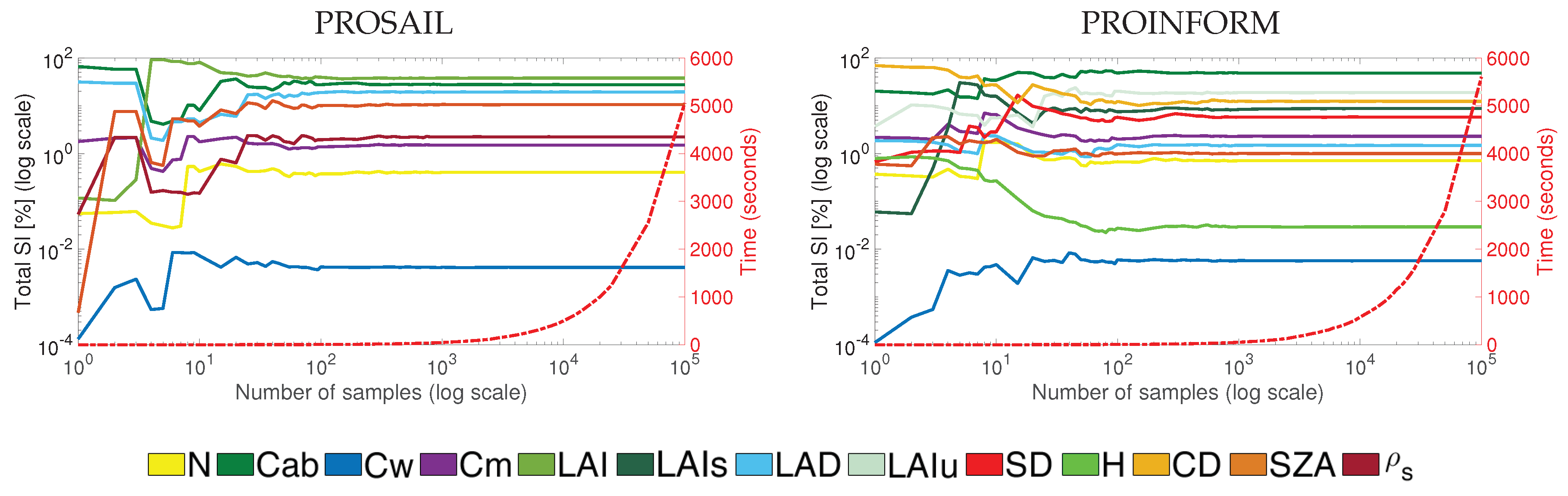
5.1. Impact of Number of Samples per RTM Variable on GSA
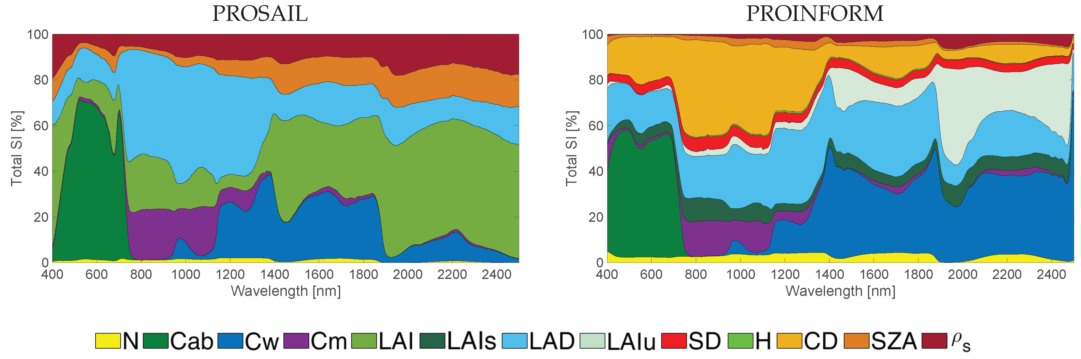
5.2. GSA Results along the 400–2500 nm Spectral Range
5.3. GSA Results for LCC-Sensitive Indices
5.4. GSA Results for LWC-Sensitive Indices
5.5. GSA Results LAI-Sensitive Indices
5.6. GSA Results for Hyperspectral Indices
6. Discussion
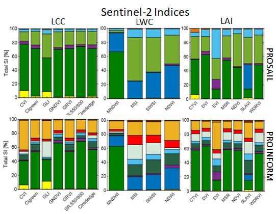
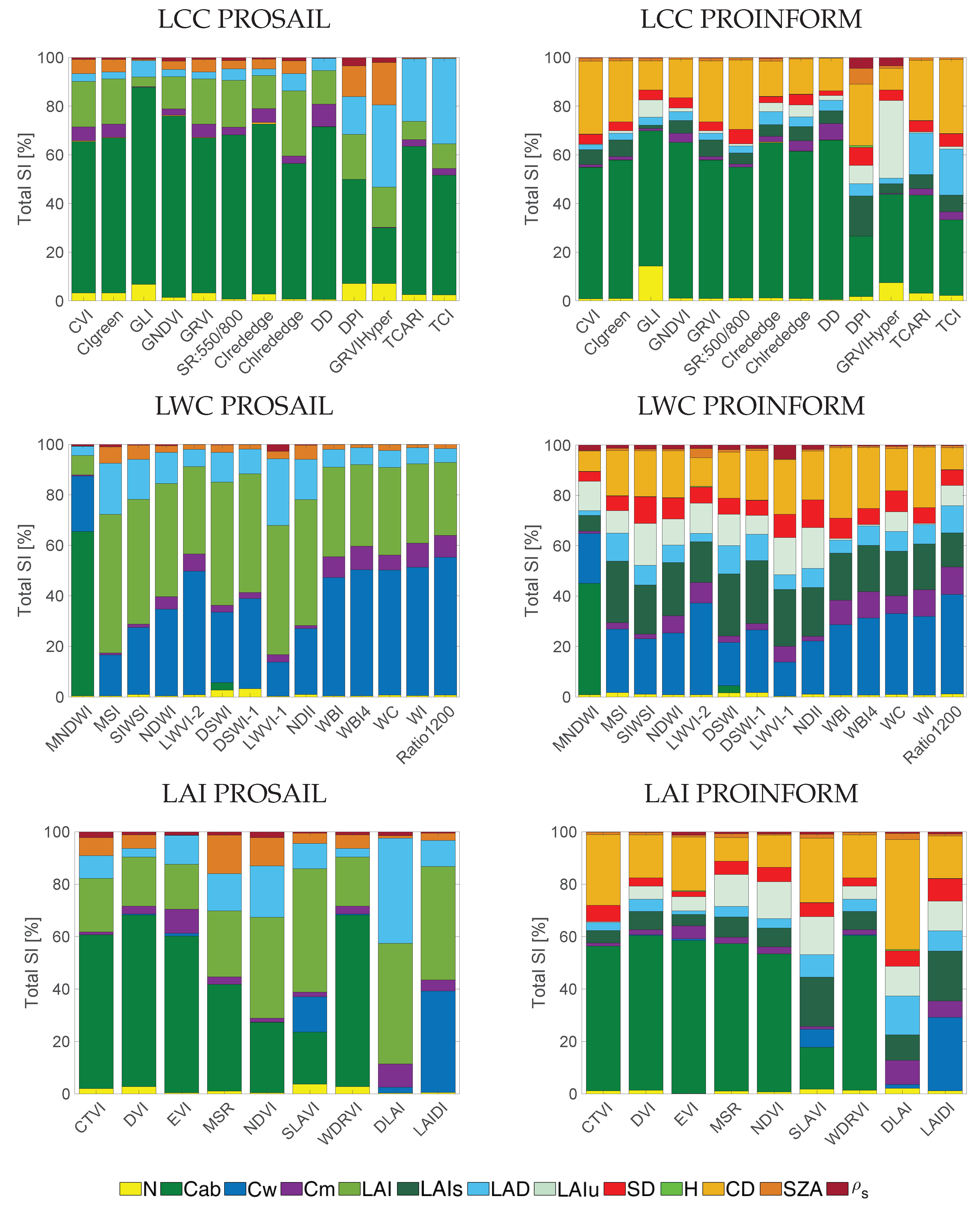
- Regarding LCC-sensitive indices, overall the most robust indices are GNDVI and SR:550/800. Those indices showed the highest total sensitivity to Cab and are thus most robust to the confounding effects of other RTMs variables. Moreover, LCC-sensitive indices are applicable to all the sensors tested including the imaging spectrometer EnMAP. For EnMAP, GNDVI showed an increase of up to 74%, as well as GLI, up to 79%. In a related study by [91], GNDVI revealed a similarly high sensitivity towards Cab as well as to LAI, but also small differences can be appreciated between both studies, probably due another GSA method used, named EFAST. When interpreting the results from a sensor point of view, then the broadband indices tend to respond more robust towards Cab estimation than the spectrometer narrowband specific indices. Hardly differences were encountered across the four tested broadband sensors. Yet, a trend can be observed, namely that these robust indices are based on exploiting the bands between 450 nm and 800 nm. This spectral range is where all the processes related to Cab absorption occur [92,93]. Most of these indices make use of only 2 bands: one sensitive band is used in the red or green region and this is compared against a more stable reference band, which is located in the NIR region [74].
- Regarding LWC-sensitive indices, overall the most robust indices are WI and Ratio1200 for PROSAIL, being the only ones that surpass 50% of and Ratio1200 for PROINFORM. These are narrowband indices available with EnMAP. Hence, for LWC-sensitive narrowband indices proved to be more effective than broadband indices. The Ratio1200 uses 3 bands located around the 1200 nm water absorption region. The influence of the SWIR band is also observed in the study by [94], as expressed by a high sensitivity of the LWVI-2 index with Cw. It is noteworthy that these indices always use a band in the NIR and SWIR regions, which is related to water absorption [95,96]. A drawback of SWIR-based indices, however, is that only a limited number of sensors cover the SWIR range. Results also suggest that multiple-band indices can be more effective than traditional 2-band indices. For instance, Ratio1200 exploits this relation using the bands: 1205 nm, 1095 nm and 1275 nm. Another remark is that the majority of the LWC-sensitive indices show superior sensitivity towards LAI, even more than some LAI-sensitive indices. This suggests that homogeneous canopies are required for the mapping of LWC [97]. The only index where we observed a good sensitivity across traditional and narrowband indices is NDWI, and also LWVI-2, which is only available for S3 when making use of SLSTR bands.
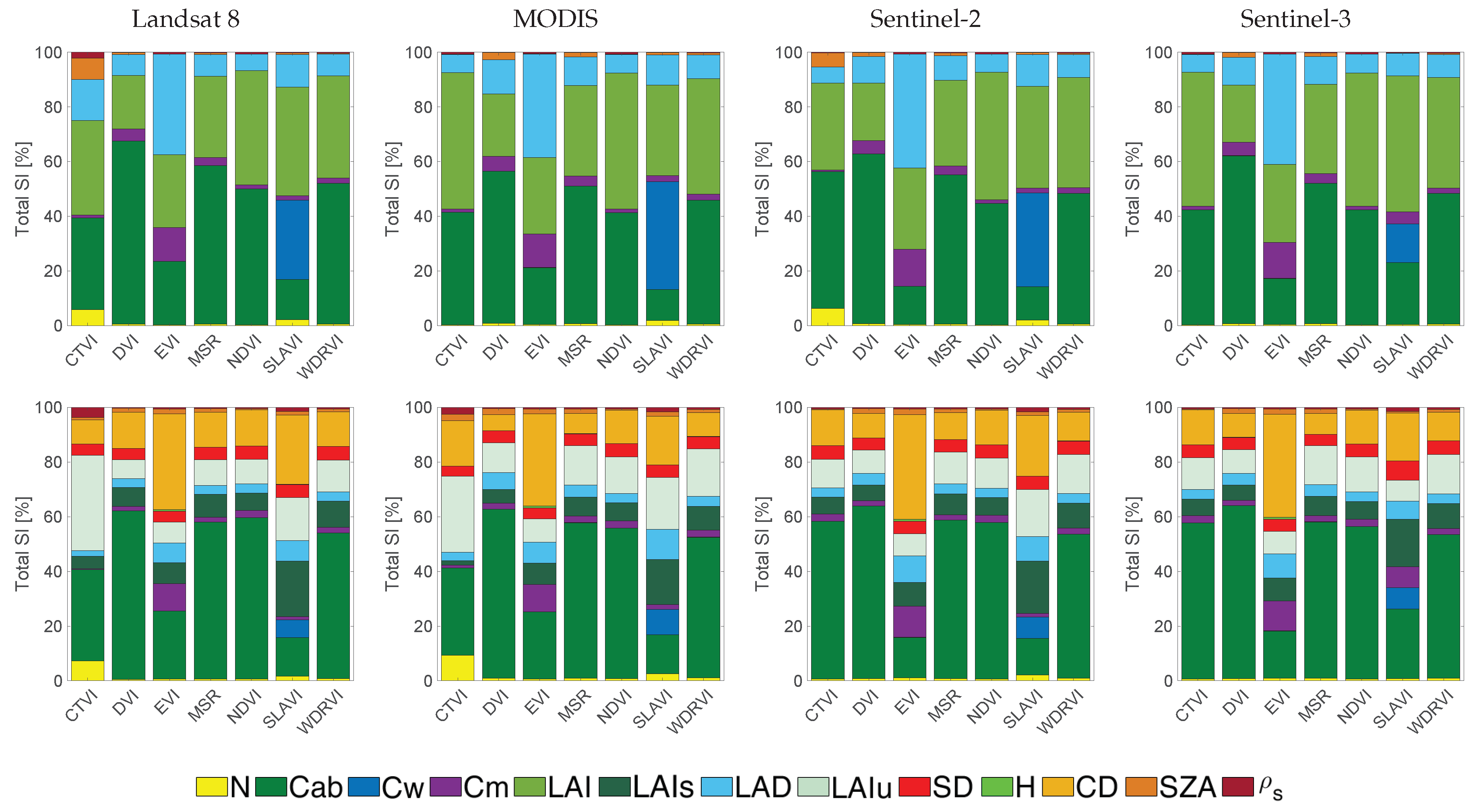
- Regarding LAI-sensitive indices, overall the most robust index is SLAVI. This index showed the highest overall sensitivity to LAI given the other PROSAIL variables and is applicable to all sensors. The narrowband spectrometer EnMAP dataset yielded somewhat better results than the broadband sensors, with the indices DLAI and LAIDI as best performing. However, when the structure is defined by many canopy variables, as is the case for PROINFORM, then LAIs is no longer the predominant variable, due to how LAI of the canopy is calculated in the model, others values such as CD, SD, and H have to be taken into consideration [88]. The greenness index NDVI reaches almost a 50% for PROSAIL. A more optimistic value is reported in [91], yet the same trend is observed in both cases: high sensitivity of LAI followed by Cab. This pattern can be observed in LAI-sensitive indices like DVI or NDVI, which are based on the comparison of a band in the red against another in the NIR [98], similar to LCC-sensitive indices. Another notable pattern is the exploiting of bands that are not influenced by Cab or water absorption, such as the DLAI or LAIDI indices, where the bands used are in the range of 970–1050 nm and 1725 nm. These kinds of indices are particularly promising for sensors that cover the SWIR range, such as EnMap [99].
Limitations and Opportunities in RTM-GSA Studies
7. Conclusions
Author Contributions
Funding
Acknowledgments
Conflicts of Interest
References
- Verrelst, J.; Rivera, J.; Veroustraete, F.; Muñoz Marí, J.; Clevers, J.; Camps-Valls, G.; Moreno, J. Experimental Sentinel-2 LAI estimation using parametric, non-parametric and physical retrieval methods—A comparison. ISPRS J. Photogramm. Remote Sens. 2015, 108, 260–272. [Google Scholar] [CrossRef]
- Dorigo, W.; Zurita-Milla, R.; de Wit, A.; Brazile, J.; Singh, R.; Schaepman, M. A review on reflective remote sensing and data assimilation techniques for enhanced agroecosystem modeling. Int. J. Appl. Earth Obs. Geoinf. 2007, 9, 165–193. [Google Scholar] [CrossRef]
- Ustin, S.; Roberts, D.; Gamon, J.; Asner, G.; Green, R. Using imaging spectroscopy to study ecosystem processes and properties. BioScience 2004, 54, 523–534. [Google Scholar] [CrossRef]
- Verrelst, J.; Schaepman, M.; Koetz, B.; Kneubuhler, M. Angular sensitivity analysis of vegetation indices derived from CHRIS/PROBA data. Remote Sens. Environ. 2008, 112, 2341–2353. [Google Scholar] [CrossRef]
- Glenn, E.; Huete, A.; Nagler, P.; Nelson, S. Relationship between remotely-sensed vegetation indices, canopy attributes and plant physiological processes: What vegetation indices can and cannot tell us about the landscape. Sensors 2008, 8, 2136–2160. [Google Scholar] [CrossRef]
- Clevers, J. Beyond NDVI: Extraction of biophysical variables from remote sensing imagery. Remote Sens. Digit. Image Process. 2014, 18, 363–381. [Google Scholar]
- Le Maire, G.; François, C.; Dufrêne, E. Towards universal broad leaf chlorophyll indices using PROSPECT simulated database and hyperspectral reflectance measurements. Remote Sens. Environ. 2004, 89, 1–28. [Google Scholar] [CrossRef]
- Le Maire, G.; François, C.; Soudani, K.; Berveiller, D.; Pontailler, J.Y.; Bréda, N.; Genet, H.; Davi, H.; Dufrêne, E. Calibration and validation of hyperspectral indices for the estimation of broadleaved forest leaf chlorophyll content, leaf mass per area, leaf area index and leaf canopy biomass. Remote Sens. Environ. 2008, 112, 3846–3864. [Google Scholar] [CrossRef]
- Xue, J.; Su, B. Significant remote sensing vegetation indices: A review of developments and applications. J. Sens. 2017, 2017, 1353691. [Google Scholar] [CrossRef]
- Corti, M.; Cavalli, D.; Cabassi, G.; Marino Gallina, P.; Bechini, L. Does remote and proximal optical sensing successfully estimate maize variables? A review. Eur. J. Agron. 2018, 99, 37–50. [Google Scholar] [CrossRef]
- Darvishzadeh, R.; Skidmore, A.; Schlerf, M.; Atzberger, C. Inversion of a radiative transfer model for estimating vegetation LAI and chlorophyll in a heterogeneous grassland. Remote Sens. Environ. 2008, 112, 2592–2604. [Google Scholar] [CrossRef]
- Verrelst, J.; Schaepman, M.E.; Malenovský, Z.; Clevers, J.G.P.W. Effects of woody elements on simulated canopy reflectance: Implications for forest chlorophyll content retrieval. Remote Sens. Environ. 2010, 114, 647–656. [Google Scholar] [CrossRef]
- Garbulsky, M.; Peñuelas, J.; Gamon, J.; Inoue, Y.; Filella, I. The photochemical reflectance index (PRI) and the remote sensing of leaf, canopy and ecosystem radiation use efficiencies. A review and meta-analysis. Remote Sens. Environ. 2011, 115, 281–297. [Google Scholar] [CrossRef]
- Jacquemoud, S.; Verhoef, W.; Baret, F.; Bacour, C.; Zarco-Tejada, P.; Asner, G.; François, C.; Ustin, S. PROSPECT + SAIL models: A review of use for vegetation characterization. Remote Sens. Environ. 2009, 113, S56–S66. [Google Scholar] [CrossRef]
- Berger, K.; Atzberger, C.; Danner, M.; D’Urso, G.; Mauser, W.; Vuolo, F.; Hank, T. Evaluation of the PROSAIL Model Capabilities for Future Hyperspectral Model Environments: A Review Study. Remote Sens. 2018, 10, 85. [Google Scholar] [CrossRef]
- Zarco-Tejada, P.; Miller, J.; Noland, T.; Mohammed, G.; Sampson, P. Scaling-up and model inversion methods with narrowband optical indices for chlorophyll content estimation in closed forest canopies with hyperspectral data. IEEE Trans. Geosci. Remote Sens. 2001, 39, 1491–1507. [Google Scholar] [CrossRef]
- Haboudane, D.; Miller, J.R.; Pattey, E.; Zarco-Tejada, P.J.; Strachan, I.B. Hyperspectral vegetation indices and novel algorithms for predicting green LAI of crop canopies: Modeling and validation in the context of precision agriculture. Remote Sens. Environ. 2004, 90, 337–352. [Google Scholar] [CrossRef]
- Le Maire, G.; Marsden, C.; Nouvellon, Y.; Stape, J.; Ponzoni, F. Calibration of a Species-Specific Spectral Vegetation Index for Leaf Area Index (LAI) Monitoring: Example with MODIS Reflectance Time-Series on Eucalyptus Plantations. Remote Sens. 2012, 4, 3766–3780. [Google Scholar] [CrossRef]
- Verrelst, J.; Camps-Valls, G.; Muñoz Marí, J.; Rivera, J.; Veroustraete, F.; Clevers, J.; Moreno, J. Optical remote sensing and the retrieval of terrestrial vegetation bio-geophysical properties—A review. ISPRS J. Photogramm. Remote Sens. 2015, 108, 273–290. [Google Scholar] [CrossRef]
- Saltelli, A.; Ratto, M.; Andres, T.; Campolongo, F.; Cariboni, J.; Gatelli, D.; Saisana, M.; Tarantola, S. Global Sensitivity Analysis: The Primer; John Wiley & Sons, Ltd.: Hoboken, NJ, USA, 2008. [Google Scholar]
- Yang, J. Convergence and uncertainty analyses in Monte-Carlo based sensitivity analysis. Environ. Model. Softw. 2011, 26, 444–457. [Google Scholar] [CrossRef]
- Nossent, J.; Elsen, P.; Bauwens, W. Sobol’sensitivity analysis of a complex environmental model. Environ. Model. Softw. 2011, 26, 1515–1525. [Google Scholar] [CrossRef]
- Xiao, Y.; Zhou, D.; Gong, H.; Zhao, W. Sensitivity of canopy reflectance to biochemical and biophysical variables. Yaogan Xuebao/J. Remote Sens. 2015, 19, 368–374. [Google Scholar] [CrossRef]
- Gu, C.; Du, H.; Mao, F.; Han, N.; Zhou, G.; Xu, X.; Sun, S.; Gao, G. Global sensitivity analysis of PROSAIL model parameters when simulating Moso bamboo forest canopy reflectance. Int. J. Remote Sens. 2016, 37, 5270–5286. [Google Scholar] [CrossRef]
- Verrelst, J.; Sabater, N.; Rivera, J.P.; Muñoz Marí, J.; Vicent, J.; Camps-Valls, G.; Moreno, J. Emulation of Leaf, Canopy and Atmosphere Radiative Transfer Models for Fast Global Sensitivity Analysis. Remote Sens. 2016, 8, 673. [Google Scholar] [CrossRef]
- Mousivand, A.; Menenti, M.; Gorte, B.; Verhoef, W. Global sensitivity analysis of the spectral radiance of a soil–vegetation system. Remote Sens. Environ. 2014, 145, 131–144. [Google Scholar] [CrossRef]
- Liu, J.; Pattey, E.; Jégo, G. Assessment of vegetation indices for regional crop green LAI estimation from Landsat images over multiple growing seasons. Remote Sens. Environ. 2012, 123, 347–358. [Google Scholar] [CrossRef]
- Zhou, G.; Ma, Z.; Sathyendranath, S.; Platt, T.; Jiang, C.; Sun, K. Canopy Reflectance Modeling of Aquatic Vegetation for Algorithm Development: Global Sensitivity Analysis. Remote Sens. 2018, 10, 837. [Google Scholar] [CrossRef]
- Dong, T.; Liu, J.; Shang, J.; Qian, B.; Ma, B.; Kovacs, J.M.; Walters, D.; Jiao, X.; Geng, X.; Shi, Y. Assessment of red-edge vegetation indices for crop leaf area index estimation. Remote Sens. Environ. 2019, 222, 133–143. [Google Scholar] [CrossRef]
- Verrelst, J.; Romijn, E.; Kooistra, L. Mapping vegetation density in a heterogeneous river floodplain ecosystem using pointable CHRIS/PROBA data. Remote Sens. 2012, 4, 2866–2889. [Google Scholar] [CrossRef]
- Verrelst, J.; Rivera, J.; Moreno, J. ARTMO’s Global Sensitivity Analysis (GSA) toolbox to quantify driving variables of leaf and canopy radiative transfer models. EARSeL eProc. 2015, 14, 1–11. [Google Scholar]
- Saltelli, A.; Annoni, P.; Azzini, I.; Campolongo, F.; Ratto, M.; Tarantola, S. Variance based sensitivity analysis of model output. Design and estimator for the total sensitivity index. Comput. Phys. Commun. 2010, 181, 259–270. [Google Scholar] [CrossRef]
- McRae, G.J.; Tilden, J.W.; Seinfeld, J.H. Global sensitivity analysis—A computational implementation of the Fourier amplitude sensitivity test (FAST). Comput. Chem. Eng. 1982, 6, 15–25. [Google Scholar] [CrossRef]
- Sobol’, I.M. On sensitivity estimation for nonlinear mathematical models. Mat. Model. 1990, 2, 112–118. [Google Scholar]
- Song, X.; Bryan, B.A.; Paul, K.I.; Zhao, G. Variance-based sensitivity analysis of a forest growth model. Ecol. Model. 2012, 247, 135–143. [Google Scholar] [CrossRef]
- Saltelli, A.; Annoni, P. How to avoid a perfunctory sensitivity analysis. Environ. Model. Softw. 2010, 25, 1508–1517. [Google Scholar] [CrossRef]
- Sobol’, I. On the distribution of points in a cube and the approximate evaluation of integrals. USSR Comput. Math. Math. Phys. 1967, 7, 86–112. [Google Scholar] [CrossRef]
- Sobol’, I.; Levitan, Y. A pseudo-random number generator for personal computers. Comput. Math. Appl. 1999, 37, 33–40. [Google Scholar] [CrossRef]
- Saltelli, A. Making best use of model evaluations to compute sensitivity indices. Comput. Phys. Commun. 2002, 145, 280–297. [Google Scholar] [CrossRef]
- Henrich, V.; Jung, A.; Götze, C.; Sandow, C.; Thürkow, D.; Gläßer, C. Development of an online indices database: Motivation, concept and implementation. In Proceedings of the 6th EARSeL Imaging Spectroscopy SIG Workshop Innovative Tool for Scientific and Commercial Environment Applications, Tel Aviv, Israel, 16–18 March 2009. [Google Scholar]
- Vincini, M.; Frazzi, E.; D’Alessio, P. A broad-band leaf chlorophyll vegetation index at the canopy scale. Precis. Agric. 2008, 9, 303–319. [Google Scholar] [CrossRef]
- Raymond Hunt, E.; Daughtry, C.S.T.; Eitel, J.U.H.; Long, D.S. Remote sensing leaf chlorophyll content using a visible band index. Agron. J. 2011, 103, 1090–1099. [Google Scholar] [CrossRef]
- Gitelson, A.A.; Viña, A.; Arkebauer, T.J.; Rundquist, D.; Keydan, G.; Leavitt, B. Remote estimation of leaf area index and green leaf biomass in maize canopies. Geophys. Res. Lett. 2003, 30, 4–7. [Google Scholar] [CrossRef]
- Ahamed, T.; Tian, L.; Zhang, Y.; Ting, K.C. A review of remote sensing methods for biomass feedstock production. Biomass Bioenergy 2011, 35, 2455–2469. [Google Scholar] [CrossRef]
- Louhaichi, M.; Borman, M.; Johnson, D. Spatially Located Platform and Aerial Photography for Documentation of Grazing Impacts on Wheat. Geocarto Int. 2001, 16. [Google Scholar] [CrossRef]
- Gitelson, A.; Kaufman, Y.; Merzlyak, M. Use of a green channel in remote sensing of global vegetation from EOS-MODIS. Remote Sens. Environ. 1996, 58, 289–298. [Google Scholar] [CrossRef]
- Gitelson, A.; Kaufman, Y.; Stark, R.; Rundquist, D. Novel algorithms for remote estimation of vegetation fraction. Remote Sens. Environ. 2002, 80, 76–87. [Google Scholar] [CrossRef]
- Xu, H. Modification of normalised difference water index (NDWI) to enhance open water features in remotely sensed imagery. Int. J. Remote Sens. 2006, 27, 3025–3033. [Google Scholar] [CrossRef]
- Datt, B. Remote sensing of water content in Eucalyptus leaves. Aust. J. Bot. 1999, 47, 909–923. [Google Scholar] [CrossRef]
- Ceccato, P.; Flasse, S.; Tarantola, S.; Jacquemoud, S.; Grégoire, J.M. Detecting vegetation leaf water content using reflectance in the optical domain. Remote Sens. Environ. 2001, 77, 22–33. [Google Scholar] [CrossRef]
- Fensholt, R.; Sandholt, I. Derivation of a shortwave infrared water stress index from MODIS near- and shortwave infrared data in a semiarid environment. Remote Sens. Environ. 2003, 87, 111–121. [Google Scholar] [CrossRef]
- Gao, B.C. NDWI—A normalized difference water index for remote sensing of vegetation liquid water from space. Remote Sens. Environ. 1996, 58, 257–266. [Google Scholar] [CrossRef]
- Zarco-Tejada, P.; Rueda, C.; Ustin, S. Water content estimation in vegetation with MODIS reflectance data and model inversion methods. Remote Sens. Environ. 2003, 85, 109–124. [Google Scholar] [CrossRef]
- Galvão, L.; Formaggio, A.; Tisot, D. Discrimination of sugarcane varieties in Southeastern Brazil with EO-1 Hyperion data. Remote Sens. Environ. 2005, 94, 523–534. [Google Scholar] [CrossRef]
- Perry, C., Jr.; Lautenschlager, L. Functional equivalence of spectral vegetation indices. Remote Sens. Environ. 1984, 14, 169–182. [Google Scholar] [CrossRef]
- Pu, R.; Gong, P.; Yu, Q. Comparative analysis of EO-1 ALI and Hyperion, and Landsat ETM+ data for mapping forest crown closure and leaf area index. Sensors 2008, 8, 3744–3766. [Google Scholar] [CrossRef] [PubMed]
- Zheng, G.; Moskal, L.M. Retrieving Leaf Area Index (LAI) Using Remote Sensing: Theories, Methods and Sensors. Sensors 2009, 9, 2719–2745. [Google Scholar] [CrossRef] [PubMed]
- Huete, A.; Didan, K.; Miura, T.; Rodriguez, E.; Gao, X.; Ferreira, L. Overview of the radiometric and biophysical performance of the MODIS vegetation indices. Remote Sens. Environ. 2002, 83, 195–213. [Google Scholar] [CrossRef]
- Ehammer, A.; Fritsch, S.; Conrad, C.; Lamers, J.; Dech, S. Statistical derivation of fPAR and LAI for irrigated cotton and rice in arid Uzbekistan by combining multi-temporal RapidEye data and ground measurements. Proc. SPIE 2010, 7824, 1–10. [Google Scholar] [CrossRef]
- Main, R.; Cho, M.A.; Mathieu, R.; O’Kennedy, M.M.; Ramoelo, A.; Koch, S. An investigation into robust spectral indices for leaf chlorophyll estimation. ISPRS J. Photogramm. Remote Sens. 2011, 66, 751–761. [Google Scholar] [CrossRef]
- Sims, D.; Gamon, J. Relationships between leaf pigment content and spectral reflectance across a wide range of species, leaf structures and developmental stages. Remote Sens. Environ. 2002, 81, 337–354. [Google Scholar] [CrossRef]
- González-Sanpedro, M.; Le Toan, T.; Moreno, J.; Kergoat, L.; Rubio, E. Seasonal variations of leaf area index of agricultural fields retrieved from Landsat data. Remote Sens. Environ. 2008, 112, 810–824. [Google Scholar] [CrossRef]
- Carlson, T.; Ripley, D. On the relation between NDVI, fractional vegetation cover, and leaf area index. Remote Sens. Environ. 1997, 62, 241–252. [Google Scholar] [CrossRef]
- Lymburner, L.; Beggs, P.; Jacobson, C. Estimation of canopy-average surface-specific leaf area using Landsat TM data. Photogramm. Eng. Remote Sens. 2000, 66, 183–191. [Google Scholar]
- Gitelson, A. Wide Dynamic Range Vegetation Index for Remote Quantification of Biophysical Characteristics of Vegetation. J. Plant Physiol. 2004, 161, 165–173. [Google Scholar] [CrossRef] [PubMed]
- Guanter, L.; Kaufmann, H.; Segl, K.; Foerster, S.; Rogass, C.; Chabrillat, S.; Kuester, T.; Hollstein, A.; Rossner, G.; Chlebek, C.; et al. The EnMAP Spaceborne Imaging Spectroscopy Mission for Earth Observation. Remote Sens. 2015, 7, 8830. [Google Scholar] [CrossRef]
- Udelhoven, T.; Delfosse, P.; Bossung, C.; Ronellenfitsch, F.; Mayer, F.; Schlerf, M.; Machwitz, M.; Hoffmann, L. Retrieving the Bioenergy Potential from Maize Crops Using Hyperspectral Remote Sensing. Remote Sens. 2013, 5, 254–273. [Google Scholar] [CrossRef]
- Locherer, M.; Hank, T.; Danner, M.; Mauser, W. Retrieval of Seasonal Leaf Area Index from Simulated EnMAP Data through Optimized LUT-Based Inversion of the PROSAIL Model. Remote Sens. 2015, 7, 10321–10346. [Google Scholar] [CrossRef]
- Bachmann, M.; Makarau, A.; Segl, K.; Richter, R. Estimating the Influence of Spectral and Radiometric Calibration Uncertainties on EnMAP Data Products—Examples for Ground Reflectance Retrieval and Vegetation Indices. Remote Sens. 2015, 7, 10689–10714. [Google Scholar] [CrossRef]
- Danner, M.; Berger, K.; Wocher, M.; Mauser, W.; Hank, T. Retrieval of Biophysical Crop Variables from Multi-Angular Canopy Spectroscopy. Remote Sens. 2017, 9, 726. [Google Scholar] [CrossRef]
- Wocher, M.; Berger, K.; Danner, M.; Mauser, W.; Hank, T. Physically-Based Retrieval of Canopy Equivalent Water Thickness Using Hyperspectral Data. Remote Sens. 2018, 10, 1924. [Google Scholar] [CrossRef]
- Hank, T.B.; Berger, K.; Bach, H.; Clevers, J.G.P.W.; Gitelson, A.; Zarco-Tejada, P.; Mauser, W. Spaceborne Imaging Spectroscopy for Sustainable Agriculture: Contributions and Challenges. Surv. Geophys. 2019, 40, 515–551. [Google Scholar] [CrossRef]
- Guanter, L.; Brell, M.; Chan, J.C.W.; Giardino, C.; Gomez-Dans, J.; Mielke, C.; Morsdorf, F.; Segl, K.; Yokoya, N. Synergies of Spaceborne Imaging Spectroscopy with Other Remote Sensing Approaches. Surv. Geophys. 2019, 40, 657–687. [Google Scholar] [CrossRef]
- Gitelson, A.A.; Keydan, G.P.; Merzlyak, M.N. Three-band model for noninvasive estimation of chlorophyll, carotenoids, and anthocyanin contents in higher plant leaves. Geophys. Res. Lett. 2006, 33. [Google Scholar] [CrossRef]
- Shibayama, M.; Salli, A.; Häme, T.; Iso-Iivari, L.; Heino, S.; Alanen, M.; Morinaga, S.; Inoue, Y.; Akiyama, T. Detecting Phenophases of Subarctic Shrub Canopies by Using Automated Reflectance Measurements. Remote Sens. Environ. 1999, 67, 160–180. [Google Scholar] [CrossRef]
- Apan, A.; Held, A.; Phinn, S.; Markley, J. Formulation and Assessment of Narrow-Band Vegetation Indices from EO-1 Hyperion Imagery for Discriminating Sugarcane Disease; Spatial Sciences Institute: Canberra, Australia, 2003; pp. 1–13. [Google Scholar]
- Hardisky, M.; Klemas, V.; Smart, R. The influence of soil salinity, growth form, and leaf moisture on the spectral radiance of Spartina alterniflora canopies. Photogramm. Eng. Remote Sens. 1983, 49, 77–83. [Google Scholar]
- Peñuelas, J.; Gamon, J.; Fredeen, A.; Merino, J.; Field, C. Reflectance indices associated with physiological changes in nitrogen- and water-limited sunflower leaves. Remote Sens. Environ. 1994, 48, 135–146. [Google Scholar] [CrossRef]
- Serrano, L.; Ustin, S.L.; Roberts, D.A.; Gamon, J.A.; Nuelas, J.P. Deriving Water Content of Chaparral Vegetation from AVIRIS Data. Remote Sens. Environ. 2000, 74, 570–581. [Google Scholar] [CrossRef]
- Underwood, E.; Ustin, S.; DiPietro, D. Mapping nonnative plants using hyperspectral imagery. Remote Sens. Environ. 2003, 86, 150–161. [Google Scholar] [CrossRef]
- Penuelas, J.; Pinol, J.; Ogaya, R.; Filella, I. Estimation of plant water concentration by the reflectance Water Index WI (R900/R970). Int. J. Remote Sens. 1997, 18, 2869–2875. [Google Scholar] [CrossRef]
- Pu, R.; Gong, P.; Biging, G.S.; Larrieu, M.R. Extraction of red edge optical parameters from Hyperion data for estimation of forest leaf area index. IEEE Trans. Geosci. Remote Sens. 2003, 41, 916–921. [Google Scholar]
- Delalieux, S.; Somers, B.; Hereijgers, S.; Verstraeten, W.; Keulemans, W.; Coppin, P. A near-infrared narrow-waveband ratio to determine Leaf Area Index in orchards. Remote Sens. Environ. 2008, 112, 3762–3772. [Google Scholar] [CrossRef]
- MATLAB. Version 9.0.0.341360 (R2016a); The MathWorks Inc.: Natick, MA, USA, 2016. [Google Scholar]
- Jacquemoud, S.; Baret, F. PROSPECT: A model of leaf optical properties spectra. Remote Sens. Environ. 1990, 34, 75–91. [Google Scholar] [CrossRef]
- Verhoef, W. Light scattering by leaf layers with application to canopy reflectance modeling: The SAIL model. Remote Sens. Environ. 1984, 16, 125–141. [Google Scholar] [CrossRef]
- Atzberger, C. Development of an invertible forest reflectance model: The INFOR-model. In Proceedings of the 20th EARSeL Symposium, Dresden, Germany, 13–16 June 2000; pp. 39–44. [Google Scholar]
- Schlerf, M.; Atzberger, C. Inversion of a forest reflectance model to estimate structural canopy variables from hyperspectral remote sensing data. Remote Sens. Environ. 2006, 100, 281–294. [Google Scholar] [CrossRef]
- Verhoef, W.; Jia, L.; Xiao, Q.; Su, Z. Unified optical-thermal four-stream radiative transfer theory for homogeneous vegetation canopies. IEEE Trans. Geosci. Remote Sens. 2007, 45, 1808–1822. [Google Scholar] [CrossRef]
- Rosema, A.; Verhoef, W.; Noorbergen, H.; Borgesius, J. A new forest light interaction model in support of forest monitoring. Remote Sens. Environ. 1992, 42, 23–41. [Google Scholar] [CrossRef]
- Zhu, W.; Huang, Y.; Sun, Z. Mapping Crop Leaf Area Index from Multi-Spectral Imagery Onboard an Unmanned Aerial Vehicle. In Proceedings of the 2018 7th International Conference on Agro-Geoinformatics (Agro-Geoinformatics), Hangzhou, China, 6–9 August 2018; pp. 1–5. [Google Scholar] [CrossRef]
- Myneni, R.; Hall, F.; Sellers, P.; Marshak, A. The interpretation of spectral vegetation indexes. IEEE Trans. Geosci. Remote Sens. 1995, 33, 481–486. [Google Scholar] [CrossRef]
- Jacquemoud, S.; Ustin, S.L.; Verdebout, J.; Schmuck, G.; Andreoli, G.; Hosgood, B. Estimating leaf biochemistry using the PROSPECT leaf optical properties model. Remote Sens. Environ. 1996, 56, 194–202. [Google Scholar] [CrossRef]
- Xiao, Y.; Zhao, W.; Zhou, D.; Gong, H. Sensitivity Analysis of Vegetation Reflectance to Biochemical and Biophysical Variables at Leaf, Canopy, and Regional Scales. IEEE Trans. Geosci. Remote Sens. 2014, 52, 4014–4024. [Google Scholar] [CrossRef]
- Hunt, E.R., Jr.; Rock, B.N. Detection of changes in leaf water content using Near- and Middle-Infrared reflectances. Remote Sens. Environ. 1989, 30, 43–54. [Google Scholar]
- Berni, J.A.; Zarco-Tejada, P.; Suárez, L.; Fereres, E. Thermal and Narrowband Multispectral Remote Sensing for Vegetation Monitoring From an Unmanned Aerial Vehicle. IEEE Trans. Geosci. Remote Sens. 2009, 47, 722–738. [Google Scholar] [CrossRef]
- Pasqualotto Vicente, N.; Delegido, J.; Van Wittenberghe, S.; Verrelst, J.; Rivera Caicedo, J.; Moreno, J. Retrieval of canopy water content of different crop types with two new hyperspectral indices: Water Absorption Area Index and Depth Water Index. Int. J. Appl. Earth Obs. Geoinf. 2018, 67, 69–78. [Google Scholar] [CrossRef]
- Delegido, J.; Verrelst, J.; Rivera, J.P.; Ruiz-Verdú, A.; Moreno, J. Brown and green LAI mapping through spectral indices. Int. J. Appl. Earth Obs. Geoinf. 2015, 35, 350–358. [Google Scholar] [CrossRef]
- Siegmann, B.; Jarmer, T.; Beyer, F.; Ehlers, M. The Potential of Pan-Sharpened EnMAP Data for the Assessment of Wheat LAI. Remote Sens. 2015, 7, 12737–12762. [Google Scholar] [CrossRef]
- Asner, G.P. Biophysical and biochemical sources of variability in canopy reflectance. Remote Sens. Environ. 1998, 64, 234–253. [Google Scholar] [CrossRef]
- Schlerf, M.; Atzberger, C. Vegetation Structure Retrieval in Beech and Spruce Forests Using Spectrodirectional Satellite Data. IEEE J. Sel. Top. Appl. Earth Obs. Remote Sens. 2012, 5, 8–17. [Google Scholar] [CrossRef]
- Deering, D.W.; Middleton, E.M.; Eck, T.F. Reflectance anisotropy for a spruce-hemlock forest canopy. Remote Sens. For. Ecosyst. 1994, 47, 242–260. [Google Scholar] [CrossRef]
- Hernández-Clemente, R.; North, P.; Hornero, A.; Zarco-Tejada, P. Assessing the effects of forest health on sun-induced chlorophyll fluorescence using the FluorFLIGHT 3-D radiative transfer model to account for forest structure. Remote Sens. Environ. 2017, 193, 165–179. [Google Scholar] [CrossRef]
- Gastellu-Etchegorry, J.P.; Lauret, N.; Yin, T.; Landier, L.; Kallel, A.; Malenovskỳ, Z.; Al Bitar, A.; Aval, J.; Benhmida, S.; Qi, J.; et al. DART: recent advances in remote sensing data modeling with atmosphere, polarization, and chlorophyll fluorescence. IEEE J. Sel. Top. Appl. Earth Obs. Remote Sens. 2017, 10, 2640–2649. [Google Scholar] [CrossRef]
- Govaerts, Y.M.; Verstraete, M.M. Raytran: A Monte Carlo ray-tracing model to compute light scattering in three-dimensional heterogeneous media. IEEE Trans. Geosci. Remote Sens. 1998, 36, 493–505. [Google Scholar] [CrossRef]
- Widlowski, J.L.; Côté, J.F.; Béland, M. Abstract tree crowns in 3D radiative transfer models: Impact on simulated open-canopy reflectances. Remote Sens. Environ. 2014, 142, 155–175. [Google Scholar] [CrossRef]
- Myneni, R.; Asrar, G.; Hall, F. A three-dimensional radiative transfer method for optical remote sensing of vegetated land surfaces. Remote Sens. Environ. 1992, 41, 105–121. [Google Scholar] [CrossRef]
- Widlowski, J.L.; Mio, C.; Disney, M.; Adams, J.; Andredakis, I.; Atzberger, C.; Brennan, J.; Busetto, L.; Chelle, M.; Ceccherini, G.; et al. The fourth phase of the radiative transfer model intercomparison (RAMI) exercise: Actual canopy scenarios and conformity testing. Remote Sens. Environ. 2015, 169, 418–437. [Google Scholar] [CrossRef]
- O’Hagan, A. Bayesian analysis of computer code outputs: A tutorial. Reliab. Eng. Syst. Saf. 2006, 91, 1290–1300. [Google Scholar] [CrossRef]
- Gómez-Dans, J.L.; Lewis, P.E.; Disney, M. Efficient Emulation of Radiative Transfer Codes Using Gaussian Processes and Application to Land Surface Parameter Inferences. Remote Sens. 2016, 8, 119. [Google Scholar] [CrossRef]
- Rivera, J.P.; Verrelst, J.; Gómez-Dans, J.; Muñoz Marí, J.; Moreno, J.; Camps-Valls, G. An Emulator Toolbox to Approximate Radiative Transfer Models with Statistical Learning. Remote Sens. 2015, 7, 9347. [Google Scholar] [CrossRef]
- Verrelst, J.; Rivera Caicedo, J.; Muñoz Marí, J.; Camps-Valls, G.; Moreno, J. SCOPE-based emulators for fast generation of synthetic canopy reflectance and sun-induced fluorescence Spectra. Remote Sens. 2017, 9, 927. [Google Scholar] [CrossRef]
- Vicent, J.; Verrelst, J.; Rivera-Caicedo, J.P.; Sabater, N.; Muñoz-Marí, J.; Camps-Valls, G.; Moreno, J. Emulation as an Accurate Alternative to Interpolation in Sampling Radiative Transfer Codes. IEEE J. Sel. Top. Appl. Earth Obs. Remote Sens. 2018, 11, 4918–4931. [Google Scholar] [CrossRef]
- Verrelst, J.; Vicent, J.; Rivera-Caicedo, J.P.; Lumbierres, M.; Morcillo-Pallarés, P.; Moreno, J. Global Sensitivity Analysis of Leaf-Canopy-Atmosphere RTMs: Implications for Biophysical Variables Retrieval from Top-of-Atmosphere Radiance Data. Remote Sens. 2019, 11, 1923. [Google Scholar] [CrossRef]
- Gabor, R.S.; Baker, A.; McKnight, D.M.; Miller, M.P. Fluorescence indices and their interpretation. Aquat. Org. Matter Fluoresc. 2014, 303–337. [Google Scholar]
- Živčák, M.; Olšovská, K.; Slamka, P.; Galambošová, J.; Rataj, V.; Shao, H.; Brestič, M. Application of chlorophyll fluorescence performance indices to assess the wheat photosynthetic functions influenced by nitrogen deficiency. Plant Soil Environ. 2015, 60, 210–215. [Google Scholar] [CrossRef]
- Van der Tol, C.; Berry, J.A.; Campbell, P.K.E.; Rascher, U. Models of fluorescence and photosynthesis for interpreting measurements of solar-induced chlorophyll fluorescence. J. Geophys. Res. 2014, 119, 2312–2327. [Google Scholar]
- Ma, S.; Zhou, Y.; Gowda, P.; Dong, J.; Zhang, G.; Kakani, V.; Wagle, P.; Chen, L.; Flynn, K.; Jiang, W. Application of the water-related spectral reflectance indices: A review. Ecol. Indic. 2019, 98, 68–79. [Google Scholar] [CrossRef]
- Lee, Z.; Carder, K.L.; Mobley, C.D.; Steward, R.G.; Patch, J.S. Hyperspectral remote sensing for shallow waters. I. A semianalytical model. Appl. Opt. 1998, 37, 6329–6338. [Google Scholar] [CrossRef] [PubMed]


| Landsat 8 | MODIS | Sentinel-2 | Sentinel-3 | EnMap | |
|---|---|---|---|---|---|
| Full Name | Moderate-resolution Imaging Spectroradiometer | Environmental Mapping and Analysis Program | |||
| Bands | 11 | 36 | 13 | OLCI: 21/SLSTR: 9 | 230 |
| Spectrum [nm] | 435–12,510 | 405–14,385 | 433–2280 | OLCI: 400–1020 SLSTR: 554–12,022 | 420–2450 |
| SR [m] | 15–100 | 250–1000 | 10–60 | 300–1200 | 30–30 |
| Inclination | 98 | 98.2 | 98.6 | 98.65 | 97.98 |
| Orbit Height [km] | 708 | 705 | 797 | 814.5 | 653 |
| Orbit Type | Sun-synchronous | Sun-synchronous circular | sun-synchronous | polar, sun-synchronous | Sun-synchronous |
| Platform | Terra/Aqua | Sentinel-2 | Sentinel-3 | ||
| Operator | NASA/USGS | NASA | ESA | EUMETSAT | DLR/GFZ |
| Launch Date | 20-02-2011 | 18-12-1999 | 23-06-2015 | 16-02-2016 | 2020 |
| Index | Abbreviation | Formula | References |
|---|---|---|---|
| LandSat 8, MODIS, Sentinel 2 and Sentinel 3 | |||
| Chlorophyll vegetation index | CVI | [41] | |
| Chlorophyll index green | CIgreen | [42,43,44] | |
| Green leaf index | GLI | [42,45] | |
| Green NDVI | GNDVI | [7,46] | |
| Green Ratio Vegetation Index | GRVI | [47] | |
| Simple Ratio 550/800 | SR:550/800 | [7] | |
| Sentinel 2 and Sentinel 3 | |||
| Chlorophyll IndexRedEdge | CIrededge | [42,43,44] |
| Index | Abbreviation | Formula | References |
|---|---|---|---|
| LandSat 8, MODIS, Sentinel 2 and Sentinel 3 | |||
| Modification of normalized difference water index | MNDWI | [48] | |
| Moisture stress index | MSI | [49,50] | |
| Shortwave infrared water stress index | SIWSI | [51] | |
| MODIS, Sentinel 2 and Sentinel 3 | |||
| Normalized difference water index | NDWI | [51,52,53] | |
| Sentinel 3 | |||
| Leaf water vegetation index-2 | LWVI2 | [54] |
| Index | Abbreviation | Formula | References |
|---|---|---|---|
| LandSat 8, MODIS, Sentinel 2 and Sentinel 3 | |||
| Corrected transformed vegetation index | CTVI | [55] | |
| Difference vegetation index | DVI | [7,56,57] | |
| Enhanced vegetation index | EVI | [42,58,59] | |
| Modified single ratio | MSR | [60,61] | |
| Normalized difference vegetation index | NDVI | [62,63] | |
| Specific leaf area vegetation index | SLAVI | [64] | |
| Wide dynamic range vegetation index | WDRVI | [44,65] |
| Index | Abbreviation | Formula | References |
|---|---|---|---|
| LCC | |||
| Chlorophyll vegetation index | CVI | [41] | |
| Chlorophyll index green | CIgreen | [42,43,44] | |
| Green leaf index | GLI | [42,45] | |
| Green NDVI | GNDVI | [7,46] | |
| Green ratio vegetation index | GRVI | [47] | |
| Simple Ratio 550/800 | SR:550/800 | [7] | |
| Chlorophyll Index Red-Edge | CIrededge | [44] | |
| Chlorophyll Red-Edge | Chlrededge | [74] | |
| Double difference index | DD | [7,60] | |
| Double peak index | DPI | [53,60] | |
| Green ratio vegetation index hyper | GRVIHyper | [75] | |
| Transformed chlorophyll absorption ratio | TCARI | [42,60] | |
| Triangular chlorophyll index | TCI | [42] | |
| LWC | |||
| Modification of normalized difference water index | MNDWI | [48] | |
| Moisture stress index | MSI | [49,50] | |
| Shortwave infrared water stress index | SIWSI | [51] | |
| Normalized difference water index | NDWI | [51,52,53] | |
| Leaf water vegetation index-2 | LWVI-2 | [54] | |
| Disease water stress index | DSWI | [54] | |
| Disease water stress index-1 | DSWI-1 | [76] | |
| Leaf water vegetation index-1 | LWVI-1 | [54] | |
| Normalized difference infrared index | NDII | [77] | |
| Water band index | WBI | [78] | |
| Water band index-4 | WBI4 | [79] | |
| Water content | WC | [80] | |
| Water Index | WI | [81] | |
| Three-band ratio 1200 | Ratio1200 | [82] | |
| LAI | |||
| Corrected Transformed Vegetation Index | CTVI | [55] | |
| Difference Vegetation Index | DVI | [7,56,57] | |
| Enhanced Vegetation Index | EVI | [42,58,59] | |
| Modified single ratio | MSR | [60,61] | |
| Normalized difference vegetation index | NDVI | [62,63] | |
| Specific Leaf Area Vegetation Index | SLAVI | [64] | |
| Wide Dynamic Range Vegetation Index | WDRVI | [44,65] | |
| Difference 1725/970 Difference LAI | DLAI | [8] | |
| Simple Ratio 1250/1050 LAI determining index | LAIDI | [83] |
| Input | Description | Unit | Min | Max |
|---|---|---|---|---|
| Leaf: PROSPECT4 | ||||
| N | Leaf structural parameter | [-] | 1 | 2.6 |
| Cab | Chlorophyll a+b content | [g/cm] | 0 | 80 |
| Cw | Equivalent water thickness | [g/cm] or [cm] | 0.001 | 0.08 |
| Cm | Dry matter content | [g/cm] | 0.001 | 0.02 |
| Canopy: SAIL and INFORM | ||||
| LAD | Leaf angle distribution | [] | 0 | 90 |
| SZA | Solar Zenith Angle | [] | 0 | 60 |
| Soil Coefficient | [-] | 0 | 1 | |
| Canopy: only SAIL | ||||
| LAI | Total leaf area index | [m/m] | 0 | 10 |
| Canopy: only INFORM | ||||
| LAIs | Single tree leaf area index | [m/m] | 0 | 10 |
| LAIu | Leaf area index of understory | [m/m] | 0 | 5 |
| SD | Stem density | [1/ha] | 0.5 | 1500 |
| H | Tree height | m | 0.5 | 30 |
| CD | Crown diameter | m | 0.1 | 10 |
© 2019 by the authors. Licensee MDPI, Basel, Switzerland. This article is an open access article distributed under the terms and conditions of the Creative Commons Attribution (CC BY) license (http://creativecommons.org/licenses/by/4.0/).
Share and Cite
Morcillo-Pallarés, P.; Rivera-Caicedo, J.P.; Belda, S.; De Grave, C.; Burriel, H.; Moreno, J.; Verrelst, J. Quantifying the Robustness of Vegetation Indices through Global Sensitivity Analysis of Homogeneous and Forest Leaf-Canopy Radiative Transfer Models. Remote Sens. 2019, 11, 2418. https://doi.org/10.3390/rs11202418
Morcillo-Pallarés P, Rivera-Caicedo JP, Belda S, De Grave C, Burriel H, Moreno J, Verrelst J. Quantifying the Robustness of Vegetation Indices through Global Sensitivity Analysis of Homogeneous and Forest Leaf-Canopy Radiative Transfer Models. Remote Sensing. 2019; 11(20):2418. https://doi.org/10.3390/rs11202418
Chicago/Turabian StyleMorcillo-Pallarés, Pablo, Juan Pablo Rivera-Caicedo, Santiago Belda, Charlotte De Grave, Helena Burriel, Jose Moreno, and Jochem Verrelst. 2019. "Quantifying the Robustness of Vegetation Indices through Global Sensitivity Analysis of Homogeneous and Forest Leaf-Canopy Radiative Transfer Models" Remote Sensing 11, no. 20: 2418. https://doi.org/10.3390/rs11202418
APA StyleMorcillo-Pallarés, P., Rivera-Caicedo, J. P., Belda, S., De Grave, C., Burriel, H., Moreno, J., & Verrelst, J. (2019). Quantifying the Robustness of Vegetation Indices through Global Sensitivity Analysis of Homogeneous and Forest Leaf-Canopy Radiative Transfer Models. Remote Sensing, 11(20), 2418. https://doi.org/10.3390/rs11202418