Assessment and Improvement of Sea Surface Microwave Emission Models for Salinity Retrieval in the East China Sea

Abstract

Accurate prediction of sea surface emission is the key for sea surface salinity retrieval from satellite microwave radiometer. In order to retrieve salinity from satellite observation, several sea surface microwave emission models have been developed based on theoretical or empirical methods and validated by in-situ measurements in different regions. However, their performances are still unclear in the Chinese coastal waters. In this study, based on two cruises measurements in the East China Sea (ECS), including the brightness temperature measured by a shipborne microwave radiometer and other auxiliary data (sea surface salinity, sea surface temperature and wind speed), the performances of different sea surface emission models are tested. The results showed that the developed models provide fairly good accuracy in predicting brightness temperature; for example, the accuracy of small perturbance/small scale approximation model (SPM/SSA), two-scale model (TSM) and empirical model is in the range from 0.6 K to 3 K. Moreover, the TSM and empirical models are further improved by optimizing the model parameters in the ECS. Finally, the sea surface salinity were retrieved from shipborne measured data based on the improved models, and the results show that the root mean square (rms) differences between retrieved and in-situ sea surface salinity is about 0.4 psu, indicating the significant improvement by the regional model parameters.

1. Introduction

Salinity is one of the most important marine parameters, which controls many processes such as physical circulations, biogeochemistry dynamics from regional to global ocean [1,2]. Although drifters and buoys, together with cruises, have accumulated large amount in-situ water salinity data in different regions, it is still difficult to monitor global ocean salinity with high temporal-spatial resolution by the in situ measurements. In the past decade, with the successful launch of the soil moisture and ocean salinity (SMOS) satellite by the European Space Agency (ESA) [3], the Aquarius/SAC-D satellite [4], and the soil moisture active passive (SMAP) satellite [5,6] by the National Aeronautics and Space Administration (NASA), global sea surface salinity (SSS) observations from space have become possible and a significant improvement has been made to understand the ocean dynamics and climate change.

The early concept of remote sensing of SSS has been demonstrated in the late 1970s with observations by Skylab [7] and two airborne L-band radiometry experiments [8,9]. At the end of 1990, two airborne microwave interferometers, the electronically scanned thinned array radiometer (ESTAR) and the scanning low-frequency microwave radiometer (SLFMR), successfully produced SSS maps in coastal areas in agreement with in-situ measurements with an accuracy of about 1 psu. Based on many experiments, the L-band is evidenced as the optimal frequency for remote sensing of SSS, which has been adopted by SMOS, Aquarius/SAC-D and SMAP. However, the sensitivity of satellite measured brightness temperature to SSS is quite low. For example, the sensitivity of vertically polarized brightness temperature to SSS variation is 0.4 to 0.8 K/psu for different observing angles and sea surface temperatures (SST), and it is only 0.2 to 0.6 K/psu for the horizontal polarization brightness temperature [10]. Thus, remote sensing of SSS requires a highly accurate retrieval model. It is widely accepted that the corrections of the sea surface and atmospheric effects are essential for remote sensing of SSS, since these effects could alter the value of sensor-measured brightness temperature and introduce errors into the SSS retrieval process. Besides the atmospheric effects, the increasing of sea surface emissivity due to the sea surface roughness and foam effects is the main source of error, which could significantly hamper the accuracy of SSS retrieval [11]. Over the past decades, the correction for sea surface roughness effects were studied based on the in-situ and airborne measurements; for example, the experiments made from a tower [12], wind and salinity experiments (WISE) [13,14], airborne Passive-Active L-band Sensor (PALS) campaign [15] and Combined Airborne Radio instruments for Ocean and Land Studies (CAROLS) campaigns [16,17]. Many rough surface emission models have also been developed based on the theoretical and empirical methods. Among these models, the small-slope approximation/small perturbation model (SSA/SPM) [18,19,20,21], two scale model (TSM) [22,23,24] and empirical/semi-empirical models [25,26] have been widely used by the research community and implemented in different satellite data processing systems. As the foam effect is significant at high wind speed conditions (above a threshold of 12 m/s) due to strong wave breaking, it has been corrected by numerous models; for example, the semi-empirical models [27,28] and radiative transfer equation (RTE) based models [29,30], which were developed to estimate the foam covered sea surface emissivity. Although many theoretical and empirical models have been developed, some problems are still unsolved. For example, the TSM originally proposed to estimate brightness temperature at higher frequencies, uses the sea surface wave spectrum by multiplying a factor of 2. However, whether this modification can be applied to L-band is still unclear, and the choice of cutoff wavenumber is arbitrary and needs to be clarified in the L-band. Moreover, the sea surface reflection of downwelling atmospheric emission is another contribution to satellite-observed brightness temperature [31], thus the determination of the cutoff wavenumber is required not only for sea surface emission but also for reflection. In addition, the widely used empirical models decouple the wind effect from SSS and SST effects, which means that the surface emission is due to a perfectly flat sea surface and the wind-roughened sea surface. The wind-roughened sea surface is associated with the increased brightness temperature (due to sea surface roughness effect), which induces regional biases when applied to different areas [32]. Furthermore, the satellite measurements of SSS are hampered by the effect of radio frequency interference (RFI) in offshore areas of China (i.e., Bohai sea, Yellow sea and East China sea), which causes a large amount of data to be discarded [33]. Thus, the compatibility of these models in coastal area of China needs to be assessed and tested in order to achieve higher accuracies of SSS from the space-borne observations.

In this paper, two cruises have been carried out in the East China Sea (ECS) to test the performance of different sea surface emissivity models at the L-band, which cover a wide range of salinity, water temperature and wind speed (19 to 34 psu, 10 to 20 °C, and 0 to 11 m/s). Moreover, based on the in situ data, the model parameters are further optimized for SSS retrieval in the ECS. In what follows, Section 2 presents the cruise experiments, Section 3 describes the data and methods used in this study, including the radiometric calibration, correction of sea surface reflected sky radiation, auxiliary data preparation and sea surface emissivity models, Section 4 presents the results and discusses the findings and finally Section 5 gives the summary.

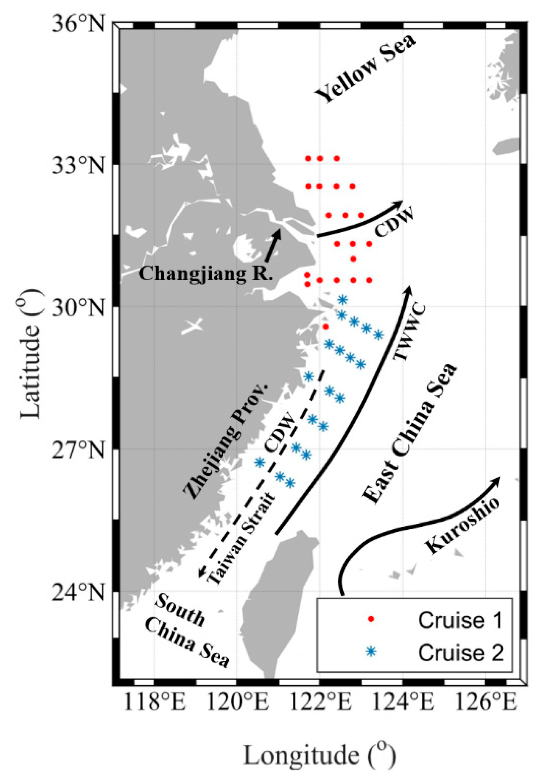
2. Cruise Experiment

The experiment was performed in the ECS with two cruises. The first cruise was conducted along the north coast of the ECS from 31 November to 4 December 2018, while the second cruise was conducted along the south coasts of the ECS from 28 April to 6 May 2019 (Figure 1). Overall, 41 stations were sampled in these two cruises experiments, of which 21 stations were covered by the first cruise and 25 stations by the second cruise. Since the two cruises were performed in two seasons, they covered a wide range of water properties (SSS 19–34 psu, SST 10–20 °C) and sea surface wind conditions (0–11 m/s), which caused a large variation of measured brightness temperature.

During the cruises, the following instruments were deployed: a dually polarimetric L-band radiometer designed and produced by Radiometrics Corporation (Figure 2a), and a stabilized platform designed and produced by Watson Corporation to keep radiometer stable during the whole cruise (Figure 2b). Moreover, to obtain the auxiliary data matched with brightness temperature measurements, two CTD (Conductivity Temperature Depth) sensors from SeaBird Electronics and RBR Corporation and a meteorological station from RM Young anemometer were used to measure SSS, SST and wind speed. The details of these instruments/experiments are briefly given below.

(1) L-band Radiometer PR-1475:

The PR-1475 is a dually polarimetric L-band radiometer designed and produced by Radiometrics Corporation. The antenna is a potter horn, which is a narrow band low sidelobe antenna, with a half-power beam width of 30° and measured side lobe levels at −23 dB. The potter horn design characteristically has sidelobes down more than 30 dB. The radiometric sensitivity is 0.1 K to 1 K depending on the integration time from 10 to 2500 msec and bandwidth of the radiometer is 25 MHz.

(2) Stabilized platform:

The stabilized platform is a particular model of the Watson product intended to hold the PR-1475 payload aligned to downward direction on a moving vehicle. This system includes a mounting bracket suited to hold the payload for rotation about its center of gravity, a mounting post made for 35 degrees of physical motion clearance and a custom counterweight designed to compensate for the PR-1475 payload.

(3) Salinity and temperature sensors:

Two different CTD sensors (SBE 37-SI MicroCAT from Sea-Bird Instruments and XR-620 from RBR Corporation) were placed on the stern and the prow of the ship. The SBE 37-SI was placed at about 1 m below the sea surface on the stern of the ship. The XR-620 was deployed to obtain the profiles of salinity and temperature at sampling stations, and it was programmed for a sampling rate of 6 Hz. Since the sampling rate was higher compared to the deployment speed of XR-620, the measured salinity in the first effective record can be recognized as sea surface salinity.

The radiometer was mounted on the stabilized platform, which was about 6 m high above the sea surface and provided dual polarization measurements of brightness temperature at 5 fixed incidence angles (16°, 26°, 36°, 45° and 60°), and the circular-shaped field of view on the sea surface has the radius in the range of 3 m to 6 m according to different incidence angles (for example, the radius of field of view is about 3 m with incidence angle at 16°). During the cruises, some stations were measured in daytime, which were hampered by sunlight. In order to avoid radiation coming from the Sun, the antenna of the radiometer was pointed away (backwards) from the sun and the radiometer’s field of view was in the shadow of the ship. At few stations, the measurements were affected by the Sun, which was removed easily because the intensity of radiation emitted by the Sun was high (~10 K or higher) and the reflectivity of the sea surface was large (in the order of 0.7). Although the effect of radio-frequency interference (RFI) is another possible source of error for the measured brightness temperature, the shipborne radiometer was deployed about 6 m above the sea surface (unlike the airborne radiometer), which could avoid potential sources of RFI. Moreover, the radiometer was pointed towards the east direction at most of the time to avoid the RFI effect from the land. In addition, it was observed that, even under the wind speeds up to 11 m/s, the foam coverage in the radiometer’s field of view was less than 5%, and thus, the foam effect was neglected in this study.

3. Data and Methods

3.1. Radiometric Calibration

The calibration equations (horizontal and vertical channels) are determined from two points: a hot and a cold targets. In this study, the sky was used as “cold target”, and an ambient temperature blackbody target as the “hot target”. The “hot target” consists of pyramidal open-cell blackbody foam in which two precision temperature sensors are embedded (Figure 3). Since the “hot target” is seen as a near-blackbody target, the value of the emitted brightness temperature is equal to its physical temperature. The brightness temperature for “cold target” is nominally 3.5 K, provided that the field of view of the radiometer is away from the galactic center and the sky is clear. To accomplish this, according to the galactic noise map [34,35], the antenna was pointed to the north, and at an elevation angle approximately 65° above the horizon.

Then the radiometer measurements were performed at different observation angles from 16° to 60° (${\theta }_i={16}^{\circ },{26}^{\circ },{36}^{\circ },{45}^{\circ }\mathrm{and} {60}^{\circ }$). The total number of the measurements was 101 for each polarization with five different incidence angles. The data possibly influenced by the RFI effect were first sorted out, and the measurements corresponding to the incidence angles outside the range of 1° larger or smaller than the incidence angles were also removed. For example, the measured brightness temperature exceeding the range of 35° to 37° for a 36° incidence angle would be rejected. After data quality control by the RFI effect and incidence angle abnormal, 18 measurements were rejected for each polarization locating at six stations, and the remain 83 high quality measurements were used for further analysis (

Table 1. Number of measurements at each incidence angle (${\theta }_i$ ) and polarization. V-pol and H-pol are the vertical and horizontal polarizations, respectively.

${\theta }_i$	16°	26°	36°	45°	60°
V-pol	12	23	28	11	9
H-pol	12	23	28	11	9

).

3.2. Correction for Sea Surface Reflection of Sky Radiation

The reflection of downward radiation (including atmospheric emission and extraterrestrial radiation) is a significant contribution to the radiometer measured brightness temperature. The extraterrestrial radiation is about 2.725 K caused by the cosmic microwave background radiation related to the Big Bang nucleosynthesis and continuum radiation [36]. Although the impact of galactic radiation (hydrogen emission and continuum radiation) could be strong when these radiation sources are limited to the specular reflection into the main antenna beam, these contaminated observations could easily be discarded because reflectivity of the sea surface is large (in the order of 0.7) and the galactic signal scattered from the sea surface is near specular reflection [10,17,37]. Thus, the steady and continuous downward radiation could be due to the cosmic background radiation plus the emission from the atmosphere. The sea surface reflected sky radiation could be estimated by the L-band radiative transfer model developed in our previous work [38]. In this model (Figure 4.), the two-scale model was used to approximate the sea surface reflected radiation towards the radiometer at different observation angles, and the downwelling atmospheric emission and radiation attenuation was obtained by using the millimeter propagation model developed by Liebe [39,40]. In addition, the profiles of the atmosphere properties were obtained from the National Center for Environmental Prediction (NCEP) FNL data, in which the whole atmosphere was divided into 26 layers, and for every layer, the gas extinction and emission were calculated with several input data including the air temperature, pressure, and relative humidity.

3.3. Auxiliary Data Preparation

The high accuracy of the input auxiliary data such as sea surface temperature, wind speed and significant wave height is required as these input data can significantly affect the accuracy of SSS retrieval. It is also necessary to obtain the brightness temperature data and auxiliary data simultaneously. In this study, together with the radiometer measurements, most of the auxiliary data were obtained by in-situ measurements with a high accuracy. The descriptions of the data processing for the auxiliary data are given below:

(1) The SSS and SST were measured by the SeaBird CTD (SBE 37-SI MicroCAT) and RBR XR-620, respectively. These two measurements were compared to ensure that the surface water properties were measured instead of the subsurface water properties. When the two measurements were not the consistent (mostly the differences less than 0.2 °C and 0.1 psu), an average value was then used.

(2) The wind speed and direction were measured by a wind monitor (RM Young anemometer, Model 05106) with the accuracy of 0.3 m/s and 3°. The anemometer was installed at a height of 8 m above the sea surface, thus the wind speed at 10 m above the sea surface was used as an input for the sea surface emission model (i.e., $U_{10}$), as approximated by Equation (1). The wind speed given at any elevation can be calculated from the friction velocity $U_{\ast }$ by:

$$U\left(z\right)=\frac{U_{\ast }}{0.4}\log \left(\frac{z}{Z_0}\right),$$

(1)

where $U_{\ast }$ is related to Z₀ by:

$$Z_0=0.0000684/U_{\ast }+0.00428U_{\ast }{}^2-0.000443,$$

(2)

and the azimuth angle is defined as ${\varphi }_w=0$ with the wind blowing towards the radiometer.

(3) Significant wave height (SWH) was obtained from the ERA5 hourly reanalysis data. Although the remote sensed SWH could achieve better accuracy than the numerical model results, only few stations could be matched to the remote sensed SWH data due to the lack of satellite SWH data in coastal regions. Thus, the SWH data from ERA5 hourly reanalysis data were used instead of the remote sensed SWH products. In fact, the ERA5 is the fifth generation ECMWF atmospheric and oceanic reanalysis production with the improved temporal-spatial resolution of 0.5 degrees in space and 1 h in time.

3.4. Sea Surface Emissivity Models

(1) Small perturbance/small scale approximation model (SPM/SSA):

In the SPM/SSA model, the Stokes vector of the emission from the sea surface is expressed as an integral over the surface directional spectrum [21] as:

$$\left[\begin{array}{c}{T}_{Bh}^{ss}\\ T_{Bv}^{ss}\end{array}\right]=SST\left(\left[\begin{array}{c}1-{\left|R_{hh}^{\left(0\right)}\right|}^2\\ 1-{\left|R_{vv}^{\left(0\right)}\right|}^2\end{array}\right]-{\displaystyle {\int }_0^{\infty }kdk{\displaystyle {\int }_0^{2\pi }W\left(k,\varphi \right)\left[\begin{array}{c}{g}_h\\ g_v\end{array}\right]d\varphi }}\right),$$

(3)

where $R_{hh}^{\left(0\right)}$ and $R_{vv}^{\left(0\right)}$ are the horizontally and vertically polarized Fresnel reflection coefficients, respectively; $W\left(k,\varphi \right)$ is the surface directional spectrum; $g_h$ and $g_v$ are the weighting functions in the formulation for correcting the reflectivity of a flat sea surface induced by small-scale waves. The weighting functions in Equation (3) are based on some theoretical understanding [18] and may require modifications based on measurements. For this, the incoherent Bragg scatter and second order correction terms were combined; the developed coordinates in [18] were modified by [21] and induced the modification of scattering coefficients. In this study, the surface directional spectrum used in the SPM/SSA model was developed by Durden and Vesecky [41] (hereafter DV spectrum). For well-developed ocean waves, the sea surface wave spectrum can be obtained as:

$$W\left(k,\varphi \right)=\frac{1}{2\pi k}S\left(k\right)\mathsf{\Phi }\left(k,\varphi \right),$$

(4)

where $S\left(k\right)$ is the omnidirectional part of the surface wave spectrum and $\mathsf{\Phi }\left(k,\varphi \right)$ is the angular portion of the spectrum. Following Durden and Vesecky, the omnidirectional part of the surface spectrum takes the form:

$$\{\begin{array}{cc}S\left(k\right)=a_0{k}^{-3}{\left(1.25k{U}_{\ast }^2/g_{\ast }\right)}^{0.225{\log }_{10}\left(k/2\right)}& k>2 \mathrm{rad}\cdot {\mathrm{m}}^{-1}\\ S\left(k\right)=b_0{k}^{-3}\exp \left[-0.74{\left(g/k{U}_{19.5}^2\right)}^2\right]& k<2 \mathrm{rad}\cdot {\mathrm{m}}^{-1}\end{array},$$

(5)

where $g^{\ast }=9.81+7.25\times {10}^{-5}{k}^2$; k is the wavenumber and $U_{\ast }$ is the friction velocity, which is defined in Equation (2); $U_{19.5}$ is the equivalent neutral wind speed given at an elevation of 19.5 m; a0 ranges from 0.004 to 0.008 and $b_0$ is selected in such a way that S(k) is continuous at k = 2 rad·m⁻¹ for a given a₀. The angular part is represented by:

$$\mathsf{\Phi }\left(k,\varphi \right)=1+c\left(1-e^{-s{k}^2}\right)\cos 2\varphi ,$$

(6)

where s is a constant set as $1.5\times {10}^{-4}$, and c is given by:

$$c=\left(\frac{1-R}{1+R}\right)\frac{2}{\left(1-D\right)},$$

(7)

with

$$R=\frac{0.003+0.00192U_{12.5}}{0.00316U_{12.5}}.$$

(8)

$$D=\frac{{\displaystyle {\int }_0^{\infty }{k}^{2}S\left(k\right)e^{-s{k}^2}dk}}{{\displaystyle {\int }_0^{\infty }{k}^{2}S\left(k\right)dk}}.$$

(9)

Following [23], some misprints of coefficients in the DV spectrum described in [41] is corrected.

(2) Two-scale model:

The two-scale model assumes that small-scale waves are rippled and superimposed on to the large-scale waves. In this model, a cutoff wavenumber k_c to determine the large-scale waves and small-scale waves is given as:

$$W\left(k,\varphi \right)=\{\begin{array}{cc}{W}_s\left(k,\varphi \right)& k>k_c\\ W_l\left(k,\varphi \right)& k<k_c\end{array}.$$

(10)

As described in the SPM/SSA model, the DV spectrum was used in this study. For small-scale waves, the Stokes vector of the emission from a local surface patch is exactly the same as Equation (3), and only the cutoff wavenumber is applied in the second terms of Equation (3). For large-scale waves, the integration is used to obtain the Stokes vector as:

$$\left[\begin{array}{c}{T}_{Bh}\\ T_{Bv}\end{array}\right]={\displaystyle {\int }_{-\infty }^{\infty }d{S}_y{\displaystyle {\int }_{-\infty }^{\cot \theta }d{S}_x}}R\left[\begin{array}{c}{T}_{Bh}^{ss}\\ T_{Bv}^{ss}\end{array}\right]\left(1-S_x\tan \theta \right)h\left(S_x\right)P\left(S_x,S_y\right),$$

(11)

where R is the rotation matrix, which rotates the coordinate from every local patch to the global coordinate, and the explicit expression of R is given in [23]; h is the hydrodynamic modulation (HM), which induces upwind/downwind asymmetry, and is also given in [23] and P is the probability density function of large-scale waves, which can be expressed as the Gaussian function as [42]:

$$P\left(S_x,S_y\right)=\frac{1}{2\pi {\sigma }_u{\sigma }_c}\exp \left(-\frac{S_x^2}{2{\sigma }_u^2}-\frac{S_y^2}{2{\sigma }_c^2}\right),$$

(12)

where ${\sigma }_u$ and ${\sigma }_c$ are variances of wave slope for upwind and crosswind directions, respectively. The variances can be calculated by a double integral over the wave and azimuth angle as:

$$S_u^2={\displaystyle {\int }_0^{\infty }dk{\displaystyle {\int }_0^{2\pi }d\varphi }}{k}^3{\cos }^2\varphi W_l\left(k,\varphi \right).$$

(13)

$$S_c^2={\displaystyle {\int }_0^{\infty }dk{\displaystyle {\int }_0^{2\pi }d\varphi }}{k}^3{\sin }^2\varphi W_l\left(k,\varphi \right).$$

(14)

(3) Empirical model:

Unlike the TSM and SPM/SSA models, the empirical model decouples the effects of SST, SSS and sea surface roughness by expanding the sea surface emission with the Taylor series function and only the first order term of the series is used to describe the sea surface roughness effect. In that case, the observed brightness temperatures at the sea surface were firstly divided into two parts due to the perfectly flat sea surface and roughness sea surface conditions as:

$$T_B^{mea}=T_{B,flat}+\mathsf{\Delta }{T}_{B,rough},$$

(15)

where

$$T_{B,flat}=\left[1-{\left|R_p\left(SSS,SST,{\theta }_i\right)\right|}^2\right]\cdot SST,$$

(16)

where R_p is the Fresnel reflection coefficient, subscript “p” stands for the polarization. It is widely accepted that $\mathsf{\Delta }{T}_{B,rough}$ is a function of WS. Camps [13] also showed that the $\mathsf{\Delta }{T}_{B,rough}$ is determined by both WS and SWH. In addition, the incidence angle is another parameter that is to be considered. Thus, the emission vector is expressed as:

$$\left[\begin{array}{c}{T}_{Bh}\\ T_{Bv}\end{array}\right]=SST\left[\begin{array}{c}1-{\left|R_{hh}^{\left(0\right)}\right|}^2\\ 1-{\left|R_{vv}^{\left(0\right)}\right|}^2\end{array}\right]+\left[\begin{array}{c}\mathsf{\Delta }{T}_h\left({\theta }_i,U_{10},SWH\right)\\ \mathsf{\Delta }{T}_v\left({\theta }_i,U_{10},SWH\right)\end{array}\right],$$

(17)

where $\mathsf{\Delta }{T}_h\left({\theta }_i,U_{10},SWH\right)$ and $\mathsf{\Delta }{T}_v\left({\theta }_i,U_{10},SWH\right)$ represent the emitted brightness temperature variations due to the sea surface roughness, and subscripts “h” and “v” denote horizontal and vertical polarizations, respectively. There are two similar methods to estimate sea surface roughness terms [25,43], and the only difference between these two methods is that the significant wave height (SWH) is introduced rather than using wind speeds (WS) directly to obtain $\mathsf{\Delta }T\left({\theta }_i,U_{10}\right)$ [44]. The sea surface roughness terms developed by Camps (hereafter Emp1) are given by:

$$\{\begin{array}{c}\mathsf{\Delta }{T}_H\approx 0.25\left(1+\frac{{\theta }_i}{94}\right)U_{10}\\ \mathsf{\Delta }{T}_V\approx 0.24\left(1-\frac{{\theta }_i}{48}\right)U_{10}\end{array},$$

(18)

where ${\theta }_i$ is the incidence angle and U₁₀ is the wind speed at 10 m above the sea surface. The other one (hereafter Emp2) is:

$$\{\begin{array}{c}\mathsf{\Delta }{T}_H\approx 0.12\left(1+\frac{{\theta }_i}{24}\right)U_{10}+0.59\left(1-\frac{{\theta }_i}{50}\right)SWH\\ \mathsf{\Delta }{T}_V\approx 0.12\left(1-\frac{{\theta }_i}{40}\right)U_{10}+0.59\left(1-\frac{{\theta }_i}{50}\right)SWH\end{array}.$$

(19)

These two empirical models are both based on the wind and salinity experiment (WISE), which were performed around the Casablanca oil rig platform, and the validity of these models in East China Sea waters remains to be explored.

4. Results and Discussion

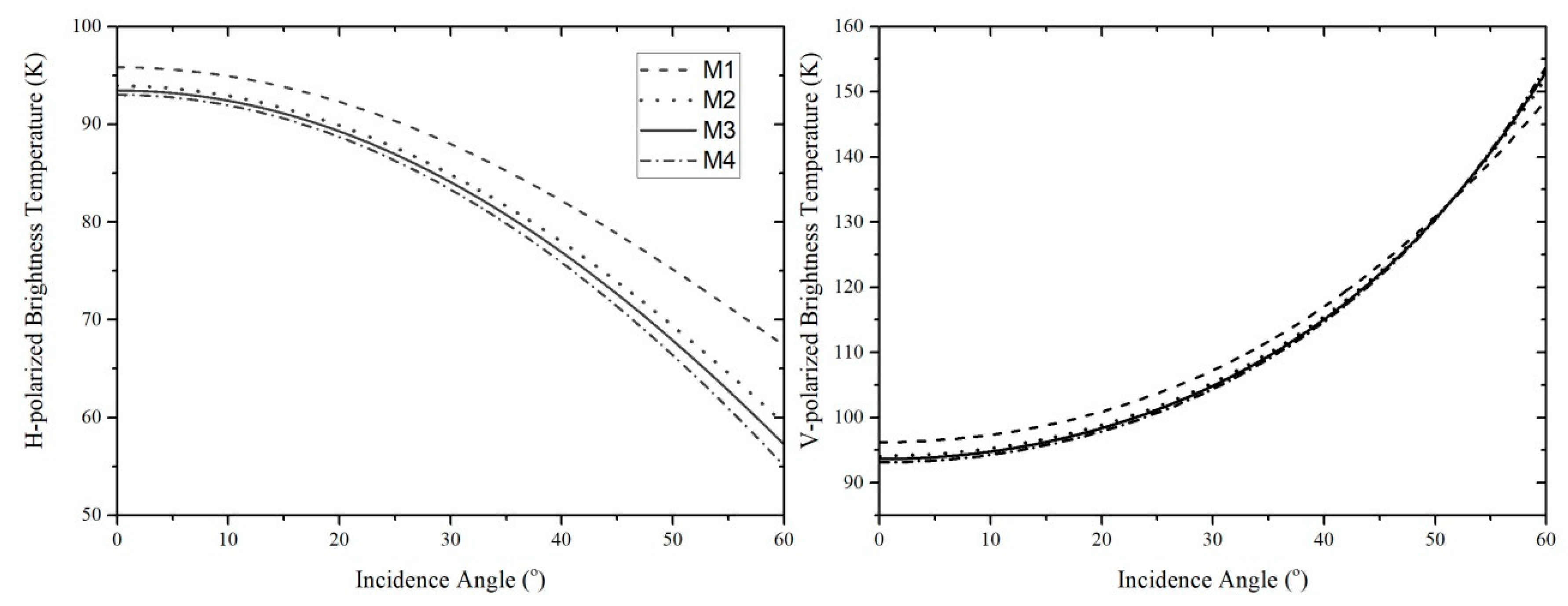
4.1. Validation of the Sea Surface Emission Models in the ECS

It is known that the prediction discrepancies of the different sea surface emission models (especially, TSM model and empirical model of [25]) are quite significant for SSS retrieval. For the TSM model, the choice of the cutoff wavenumber and the factor a0 can affect the prediction of brightness temperature significantly. The a0 value is always assumed to vary from 0.004 to 0.008, and in some studies, the DV spectrum is multiplied with a factor of 2 [16,32,44]. In this paper, the TSM model with four typical combinations of factors was used to predict the brightness temperature and compare with the in-situ measured data, and the choices of the factor and a0 values are shown in

Table 2. Parameters of the two scale model (TSM).

	Factor	${\mathit{a}}_0$
M1	2	0.008
M2	1	0.008
M3	1	0.006
M4	1	0.004

. The influence of different factor and a0 values on the predicted brightness temperature is shown in Figure 5, in which the SST and SSS were fixed as 15 °C and 35 psu, and the cutoff wavenumber was set as $k_c=k_0/3$. Clearly, the predicted brightness temperature obtained from the model M1 (DV spectrum multiplied with the factor 2, hereafter DV2) is higher than those from the models M2, M3 and M4, especially for the horizontal polarization component. Comparing to vertical polarization, the horizontal polarization is sensitive to the wave spectrum, and the differences among the models M1, M2, M3 and M4 can reach up to 2 K at nadir, and increase to 10 K with an incidence angle at 60°, which is too large for SSS retrieval. The differences between the models M1, M2, M3 and M4 are less than 2 K for vertical polarization, which is reasonable because the vertical polarized brightness temperature is less influenced by the sea surface roughness effect. Although the differences are small for vertical polarization, it is still too large for SSS retrieval. Thus, these factors need to be determined by fitting the model predictions to the in-situ measurements. On the other hand, due to the limited brightness temperature measurements in coastal waters of China, the regional bias of the empirical model in the ECS is still unclear and needs to be examined.

Table 3. Comparison of the model predicted and in-situ measured brightness temperature. V-pol: vertical polarization; H-pol: horizontal polarization.

	rms Difference (K)		$\mathbf{\Delta }{\mathit{T}}_{\mathit{B}} \mathbf{Std} \left(\mathbf{K}\right)$		Biases (K)
	H-pol	V-pol	H-pol	V-pol	H-pol	V-pol
M1	1.35	0.93	1.03	0.89	−0.88	−0.28
M2	0.60	0.50	0.46	0.39	−0.39	−0.31
M3	0.47	0.57	0.42	0.52	0.20	−0.25
M4	2.99	1.69	1.49	1.70	2.60	0.08
SPM/SSA	1.13	0.71	0.73	0.71	−0.86	0.08
EMP1	1.06	0.73	1.01	0.71	−0.34	−0.19
EMP2	1.05	0.78	0.97	0.73	−0.41	−0.27

presents the results for different sea surface emission models obtained by comparing the model-predicted and in situ brightness temperatures. The M4 model had the largest root-mean-square difference (rms; up to 3 K) for horizontally polarized brightness temperature, which could lead to 3 psu or a higher bias in SSS retrieval. Although the wave spectrum was multiplied with a factor of 2 to fit with the measured brightness temperature at higher frequencies [18], as done previously [16,32], the DV2 spectrum would overestimate the brightness temperature values. The rms values were the lowest for horizontally polarized brightness temperature with the M2 model and for vertically polarized brightness temperature with the M3 model. According to the mean biases, the M2 model slightly underestimated the brightness temperature, whereas the M3 model overestimated the brightness temperature. The underestimation or overestimation of the brightness temperature by these models might be attributed to the choice of cutoff wavenumber. Thus, the cutoff wavenumber needs to be considered in the model (as discussed in a later section). Furthermore, the empirical models developed based on the WISE campaigns show the regional biases in the ECS, and the coefficients in these models also need to be optimized.

4.2. Optimization of the Emission Models for ECS Waters

4.2.1. The Choice of k_c

The choice of k_c is rather arbitrary in previous studies; for example, $k_c=k_0/4$, $k_c=k_0/5$ and $k_c=k_0/10$ according to [32], [45] and [24], respectively. The kc values were given in the range of k₀/10 to k₀/3. The reason is that, as shown in [32], for the range of k₀/10 to k₀/3, the effect of k_c on the predicted brightness temperature is small or even negligible. In addition, when using the DV2 spectrum, the difference caused by the cutoff wavenumber is less than 0.4 K with the incidence angle at 30° and 40°. Thus, $k_c=k_0/3$, $k_c=k_0/5$ and $k_c=k_0/10$ were tested in this study.

As shown in Figure 6, the horizontally polarized brightness temperatures had higher correlations with a0 and cutoff wavenumbers than the vertically polarized brightness temperatures. Moreover, the brightness temperature was underestimated when a0 was set as 0.004, especially for horizontal polarization, and when a0 was 0.006, or a0 = 0.008 together with k_c = k₀/3, the errors were relatively small compared to other combinations of a0 and kc values. The performances of the TSM model with different a0 and kc values are shown in

Table 4. Comparison of the model predicted and in-situ measured brightness temperatures. V-pol: vertical polarization; H-pol: horizontal polarization.

	rms Difference (K)		$\mathbf{\Delta }{\mathit{T}}_{\mathit{B}} \mathbf{Std} \left(\mathbf{K}\right)$		Biases (K)
	H-pol	V-pol	H-pol	V-pol	H-pol	V-pol
a0 = 0.006, $k_c=k_0/10$	0.39	0.37	0.39	0.37	0.07	0.02
a0 = 0.006, $k_c=k_0/5$	0.45	0.40	0.41	0.37	−0.20	−0.17
a0 = 0.006, $k_c=k_0/3$	0.59	0.49	0.46	0.39	−0.39	−0.31
a0 = 0.008, $k_c=k_0/3$	0.47	0.57	0.42	0.52	0.20	−0.25

, by comparison between the predicted and in situ brightness temperatures. The results show that a0 = 0.006 with $k_c=k_0/10$ fit the in situ values best with the rms values of 0.39 K and 0.37 K for horizontally polarized and vertically polarized brightness temperatures, respectively. In addition, the biases and standard deviations were also small when a0 = 0.006 and $k_c=k_0/10$. Although the rms values were similar for different a0 and k_c values, the biases for horizontally and vertically polarized brightness temperatures had a significant influence on the SSS retrieval using these models.

4.2.2. Adjustment of the Empirical Model for the ECS

Following Equations (17)–(19), for every incidence angle, the sensitivity of $\mathsf{\Delta }{T}_{B,rough}$ to WS (or SWH) is represented by the slope of linear regression of $\mathsf{\Delta }{T}_{B,rough}$ to WS (or SWH). Generally, $\mathsf{\Delta }{T}_{B,rough}$ can be expressed as:

$$\mathsf{\Delta }{T}_{B,rough}=a\cdot S_{WS}\left({\theta }_i\right)\cdot U_{10}+c,$$

(20)

$$\mathsf{\Delta }{T}_{B,rough}=a\cdot S_{WS}\left({\theta }_i\right)\cdot U_{10}+b\cdot S_{SWH}\left({\theta }_i\right)\cdot SWH+c,$$

(21)

where $S_i\left({\theta }_i\right)$ is the sensitivity of $\mathsf{\Delta }{T}_{B,rough}$ to WS (or SWH), i = 1, 2 and 3 and c is the offset. In this study, although all the in situ data were used, the number of measured brightness temperature was still small for different incidence angles. Thus, the wind speed sensitivity was obtained based on the previous studies. It should be noted that the fitted sensitivity of vertically polarized brightness temperature to wind speed from different campaigns was quite different. For example, at 20° and 30° incidence angles, the vertical polarization sensitivity to wind speed, as derived by the WISE, was half as it was obtained from the PALS and Hollinger’s data. It decreased to −0.03 with the incidence angle at 50°, whereas it was 0.22 from the PALS dataset. This could be attributed to the discrepancies in the dielectric constant model used to compute the flat sea surface brightness temperature (Equation (16)). The dielectric constant model used in this study was from Klein and swift [46], which is the same used in [13]. Thus, the wind speed sensitivity at different incidence angles was exactly the same as [13].

A linear regression method was used to obtain the coefficients in Equations (20) and (21). The relationships of $\mathsf{\Delta }{T}_{B,rough}$ with wind speeds and incidence angles are shown in Figure 7. Overall, the $\mathsf{\Delta }{T}_{h,rough}$ shows a good correlation with sensitivity and wind speed, and the vertical polarization variations show a lower sensitivity to wind speed compared to the horizontal polarization, which were consistent with the previous studies [10]. This might be attributed to the fact that the vertically polarized brightness temperature was less influenced by the WS and roughness. It should be noted that, for both polarizations, the brightness temperature variations did not fit well with incidence angle at 60° (green points), this was particularly more evident for horizontal polarization. When the data at a 60° incidence angle were excluded, the correlation coefficients between $\mathsf{\Delta }{T}_{h,rough}$ and wind speed (multiplying sensitivity) increased from 0.78 to 0.88. Although the brightness temperature measured at high incidence angles were less used for SSS retrieval, further study is still needed to examine the variation of sea surface roughness induced brightness temperature at low incidence angles and high incidence angles separately. From this analysis, the optimized $\mathsf{\Delta }{T}_{h,rough}$ and $\mathsf{\Delta }{T}_{v,rough}$ models for the ECS are given by:

$$\begin{array}{l}\mathsf{\Delta }{T}_{h,rough}=0.57692S_{h,WS}\left({\theta }_i\right)U_{10}+1.583S_{h,SWH}\left({\theta }_i\right)SWH+0.30231\\ \mathsf{\Delta }{T}_{v,rough}=0.36248S_{v,WS}\left({\theta }_i\right)U_{10}+0.77851S_{v,SWH}\left({\theta }_i\right)SWH-0.311863\end{array},$$

(22)

where S is the sensitivity of different parameters (i.e., WS and SWH), subscripts “h” and “v” represent horizontal and vertical polarizations, respectively. It should be noted that the sensitivity of horizontally polarized brightness temperature to SWH obtained from [13] is notably different from that of [25] (θ/142 comparing to 1 − θ/50). For example, when the incidence angle at 60°, the sensitivity was 0.4225 and −0.2 from these two models. In order to fit well with the measurements, these two sensitivities were both tested in this study, and the results showed that the sensitivity from [13] fitted well with the measurements, and finally θ/142 was used in Equation (22).

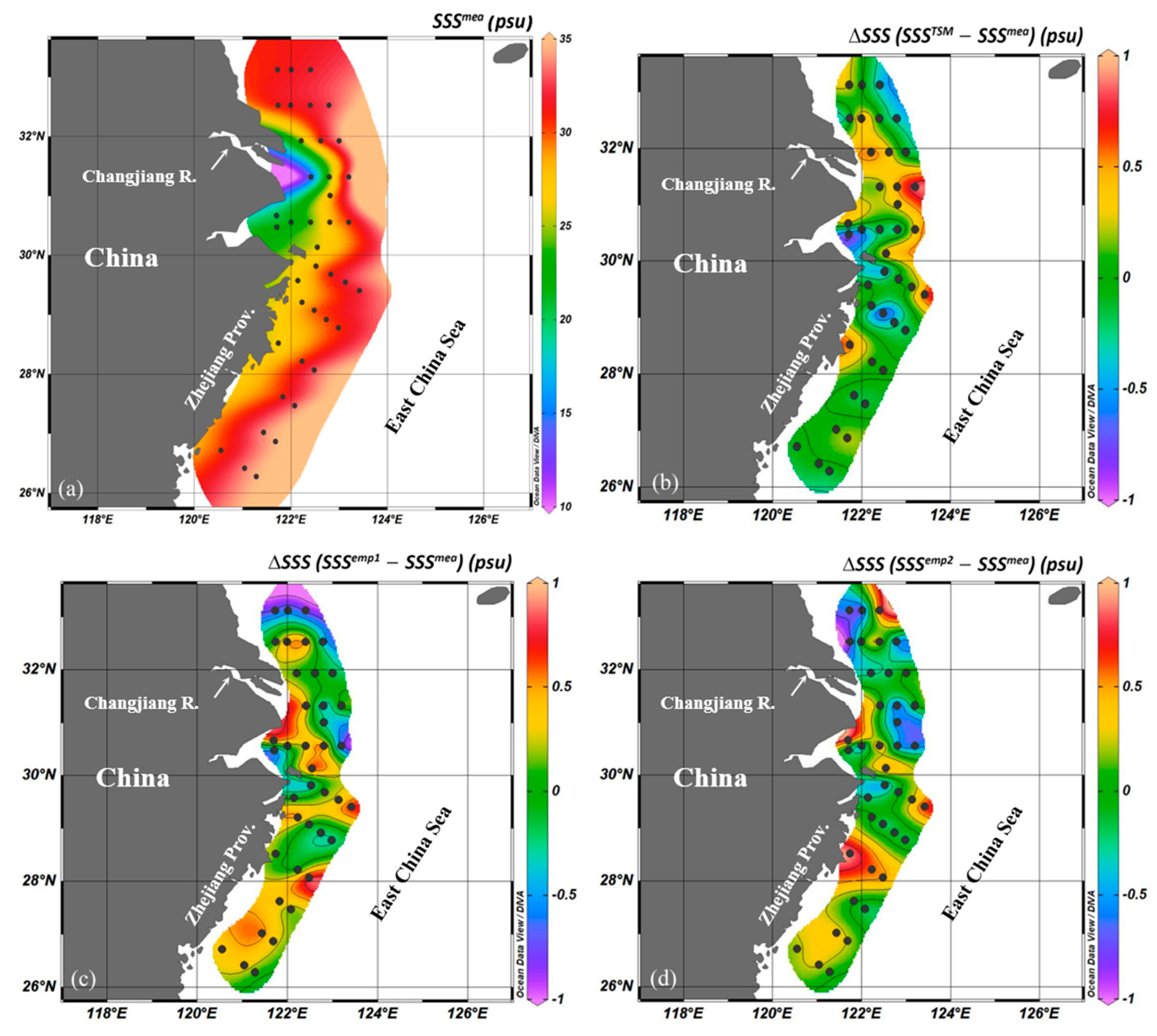
4.2.3. Comparison of the Retrieved Sea Surface Salinity using Different Models

For SSS retrieval, the iterative Levenberg and Marquard method was used, which is fully described in the literature [47,48]. The L–M method was performed by minimizing the cost function defined as:

$${\chi }^2={\displaystyle \sum _i\frac{{\left(T_{Bi}^{mea}-T_{Bi}^{\mathrm{mod}}\right)}^2}{{\sigma }_{T_{Bi}^{}}^2}}+\frac{{\left(SSS-SS{S}^{prior}\right)}^2}{{\sigma }_{SSS}^2},$$

(23)

where $T_{Bi}^{mea}$ and $T_{Bi}^{\mathrm{mod}}$ are the measured and model-predicted brightness temperatures, respectively; ${\sigma }_{T_{Bi}^{}}^2$ is the expected error variance of the measurements; $SS{S}^{prior}$ represents the priori value of SSS and ${\sigma }_{SSS}^2$ is the expected error variances of the priori SSS. The horizontally polarized brightness temperature, vertically polarized brightness temperature and the first Stokes parameter (i.e., (T_BH + T_BV)/2) can all be used to retrieve SSS (Equation. (23)). It is known that using the first Stokes parameter can achieve a higher sensitivity to SSS, however, when the forward model overestimates or underestimates the sea surface emission, the error of retrieved SSS would be larger. In this paper, three models were used to retrieve SSS: (1) TSM with a0 = 0.006 and $k_c=k_0/10$, (2) modified EMP1 and (3) modified EMP2 (the results are reported in

Table 5. A comparison of errors obtained between the retrieved and in-situ measured sea surface salinity (SSS) from shipborne radiometric measurements (N = 41).

	$\mathbf{RMS} \mathbf{\Delta }\mathit{S}\mathit{S}\mathit{S} \left(\mathbf{psu}\right)$	$\mathbf{Std}\mathbf{\Delta }\mathit{S}\mathit{S}\mathit{S} \left(\mathbf{psu}\right)$	$\mathbf{Biases} \mathbf{\Delta }\mathit{S}\mathit{S}\mathit{S} \left(\mathbf{psu}\right)$
TSM	0.38	0.37	0.04
EMP1	0.44	0.43	0.08
EMP2	0.48	0.48	−0.01

). It can be seen that the RMS of the retrieved SSS was about 0.4 psu for all three models, but the modified TSM model had the highest accuracy. The lower performance of the EMP models compared to the TSM model might be due to the fewer in-situ measurements used to improve the empirical model. As mentioned in Section 4.2, the $\mathsf{\Delta }{T}_{B,rough}$ needs to be calculated separately at low and high incidence angles in order to achieve the higher accuracy.

The spatial distributions of retrieval errors are shown in Figure 8. Clearly, the accuracy of retrieved SSS using the modified TSM model was higher than the two empirical models, especially at stations in the vicinity of the coast. For these stations, the shallow water was one of the factors that affected the sea surface roughness contributions, since shallow water waves were significantly affected by the seabed topography in these coastal areas. Moreover, the error of the SWH was another source, which hampered the accuracy of model prediction and SSS retrieval. In this study, the spatial resolution of the SWH data obtained from the ECMWF ERA-5 reanalysis dataset was 0.5° × 0.5°, which was too coarse to match the field of view of radiometer. Thus, in order to derive an empirical model with high accuracy, the SWH should be measured simultaneously with the radiometer measurement.

5. Conclusions

Satellite remote sensing of SSS is based on the variation of sea surface emission caused by the change of salinity, but this method generally assumes that the sea surface is perfectly flat. However, in the real world, the sea surface is always rough, and sea surface emission is significantly affected by the sea surface roughness. Thus, one of the most important issues in remote sensing of SSS is to remove the contribution of sea surface roughness on sea surface emission. In this study, two cruise experiments were performed in the ECS to assess and improve the sea surface microwave emission models in the ECS. To obtain the brightness temperature of the sea surface, the contributions of surface reflected downwelling sky radiations including cosmic microwave background radiation and atmospheric emission were first removed by using a developed radiative transfer model. Based on the in situ brightness temperature and auxiliary data (including SSS, SST, wind speed and direction and SWH), the performances of different emission models including TSM, SPM and SSA and empirical models were examined. The results showed that the accuracy of these models varied from 0.6 K to 3 K. The accuracy of TSM was influenced by the choices of parameters in the surface wave spectrum. The error of TSM could reach up to 0.6 K for a0 = 0.006 and decrease to 3 K with the wave spectrum multiplied with a factor 2, and the accuracy of SSA/SPM and empirical models were quite similar, which were 1.1 K and 0.8 K for horizontally and vertically polarized brightness temperatures, respectively.

The validation in this study showed that the existing models performed poorly in the ECS and required to be optimized for regional applications. For the TSM, it is well known that the accuracy is affected by the choice of the parameters a0 and cutoff wavenumber k_c. It was found that with a0 = 0.006 and k_c = k₀/10, the brightness temperature could be fairly accurately predicted with an error less than 0.4 K for both polarizations. Furthermore, the empirical models were improved to be applicable for the ECS by optimizing the model parameters, and the brightness temperature variation as a function of both wind speed and SWH was also established. The results showed that the sea surface roughness induced brightness temperature variations were well fitted by wind speed at low incidence angles, especially for horizontal polarization, with the correlation coefficient of 0.88. At large incidence angles, the brightness temperature variations also showed a good correlation with sensitivity and wind speed. However, when all data were used, the accuracy of model prediction became lower, which needs further study to improve the empirical model performance. Based on SSS retrievals with the improved models using shipborne brightness temperature data, it was found that that the modified TSM retrieved SSS with an RMS and standard deviation around 0.4 psu. Compared to the modified TSM model, the accuracy of retrieved SSS using the EMP model was relatively low, which might be caused by the influence of seabed topography on the surface wave spectrum and the coarse resolution of the input SWH data.

References

1. Murtugudde, R.; Busalacchi, A.J. Salinity effects in a tropical ocean model. J. Geophys. Res. Ocean. 1998, 103, 3283–3300. [Google Scholar] [CrossRef] [Green Version]
2. Schanze, J.J.; Schmitt, R.W.; Yu, L.L. The global oceanic freshwater cycle: A State-of-the-art quantification. J. Mar. Res. 2010, 68, 569–595. [Google Scholar] [CrossRef]
3. Kerr, Y.H.; Waldteufel, P.; Wigneron, J.; Delwart, S.; Cabot, F.; Boutin, J.; Escorihuela, M.; Font, J.; Reul, N.; Gruhier, C. The SMOS mission: New tool for monitoring key elements ofthe global water cycle. Proc. IEEE 2010, 98, 666–687. [Google Scholar] [CrossRef]
4. Le Vine, D.M.; Lagerloef, G.S.E.; Torrusio, S.E. Aquarius and Remote Sensing of Sea Surface Salinity from Space. Proc. IEEE 2010, 98, 688–703. [Google Scholar] [CrossRef] [Green Version]
5. Entekhabi, D.; Njoku, E.G.; O’Neill, P.E.; Kellogg, K.H.; Crow, W.T.; Edelstein, W.N.; Entin, J.K.; Goodman, S.D.; Jackson, T.J.; Johnson, J.T. The soil moisture active passive (SMAP) mission. Proc. IEEE 2010, 98, 704–716. [Google Scholar] [CrossRef]
6. Piepmeier, J.R.; Focardi, P.; Horgan, K.A.; Knuble, J.; Ehsan, N.; Lucey, J.; Brambora, C.; Brown, P.R.; Hoffman, P.J.; French, R.T. SMAP L-band microwave radiometer: Instrument design and first year on orbit. IEEE Trans. Geosci. Remote Sens. 2017, 55, 1954–1966. [Google Scholar] [CrossRef]
7. Lerner, R.M.; Hollinger, J.P. Analysis of 1.4 GHz radiometric measurements from Skylab. Remote Sens. Environ. 1977, 6, 251–269. [Google Scholar] [CrossRef]
8. Thomann, G.C. Experimental results of the remote sensing of sea-surface salinity at 21-cm wavelength. IEEE Trans. Geosci. Electron. 1976, 14, 198–214. [Google Scholar] [CrossRef]
9. Blume, H.C.; Kendall, B.M.; Fedors, J.C. Measurement of ocean temperature and salinity via microwave radiometry. Bound. Layer Meteorol. 1978, 13, 295–308. [Google Scholar] [CrossRef]
10. Yueh, S.H.; West, R.; Wilson, W.J.; Li, F.K.; Njoku, E.G.; Rahmat-Samii, Y. Error sources and feasibility for microwave remote sensing of ocean surface salinity. IEEE Trans. Geosci. Remote Sens. 2001, 39, 1049–1060. [Google Scholar] [CrossRef] [Green Version]
11. Hwang, P.A.; Reul, N.; Meissner, T.; Yueh, S.H. Ocean surface foam and microwave emission: Dependence on frequency and incidence angle. IEEE Trans. Geosci. Remote Sens. 2019, 57, 8223–8234. [Google Scholar] [CrossRef]
12. Hollinger, J.P. Passive Microwave Measurements of the Sea Surface. J. Geophys. Res. 1970, 75, 5209–5213. [Google Scholar] [CrossRef]
13. Camps, A.; Font, J.; Vall-Llossera, M.; Gabarro, C.; Corbella, I.; Duffo, N.; Torres, F.; Blanch, S.; Aguasca, A.; Villarino, R. The WISE 2000 and 2001 field experiments in support of the SMOS mission: Sea surface L-band brightness temperature observations and their application to sea surface salinity retrieval. IEEE Trans. Geosci. Remote Sens. 2004, 42, 804–823. [Google Scholar] [CrossRef]
14. Etcheto, J.; Dinnat, E.P.; Boutin, J.; Camps, A.; Miller, J.; Contardo, S.; Wesson, J.; Font, J.; Long, D.G. Wind speed effect on L-band brightness temperature inferred from EuroSTARRS and WISE 2001 field experiments. IEEE Trans. Geosci. Remote Sens. 2004, 42, 2206–2213. [Google Scholar] [CrossRef]
15. Yueh, S.H.; Dinardo, S.J.; Fore, A.G.; Li, F.K. Passive and Active L-Band Microwave Observations and Modeling of Ocean Surface Winds. IEEE Trans. Geosci. Remote Sens. 2010, 48, 3087–3100. [Google Scholar] [CrossRef]
16. Martin, A.C.H.; Boutin, J.; Hauser, D.; Reverdin, G.; Parde, M.; Zribi, M.; Fanise, P.; Chanut, J.; Lazure, P.; Tenerelli, J. Remote Sensing of Sea Surface Salinity from CAROLS L-Band Radiometer in the Gulf of Biscay. IEEE Trans. Geosci. Remote Sens. 2012, 50, 1703–1715. [Google Scholar] [CrossRef]
17. Martin, A.C.H.; Boutin, J.; Hauser, D.; Dinnat, E.P. Active-passive synergy for interpreting ocean L-band emissivity: Results from the CAROLS airborne campaigns. J. Geophys. Res. Ocean. 2015, 119, 4940–4957. [Google Scholar] [CrossRef]
18. Yueh, S.H.; Kwok, R.; Nghiem, S.V. Polarimetric scattering and emission properties of targets with reflection symmetry. Radio Sci. 1994, 29, 1409–1420. [Google Scholar] [CrossRef] [Green Version]
19. Voronovich, A. Small-slope approximation for electromagnetic wave scattering at a rough interface of two dielectric half-spaces. Waves Random Media 1994, 4, 337–368. [Google Scholar] [CrossRef]
20. Irisov, V.G. Small-slope expansion for thermal and reflected radiation from a rough surface. Waves Random Media 1997, 7, 1–10. [Google Scholar] [CrossRef]
21. Johnson, J.T.; Zhang, M. Theoretical study of the small slope approximation for ocean polarimetric thermal emission. IEEE Trans. Geosci. Remote Sens. 1999, 37, 2305–2316. [Google Scholar] [CrossRef]
22. Wu, S.T.; Fung, A.K. A non-coherent model for microwave emission and backscattering from the sea surface. J. Geophys. Res. 1972, 77, 5917–5929. [Google Scholar] [CrossRef]
23. Yueh, S.H. Modeling of Wind Direction Signals in Polarimetric Sea Surface Brightness Temperatures. IEEE Trans. Geosci. Remote Sens. 1997, 35, 1400–1418. [Google Scholar] [CrossRef]
24. Johnson, J.T. An efficient two-scale model for the computation of thermal emission and atmospheric reflection from the sea surface. IEEE Trans. Geosci. Remote Sens. 2006, 44, 560–568. [Google Scholar] [CrossRef]
25. Gabarró, C.; Font, J.; Camps, A.; Vall-Llossera, M.; Julià, A. A new empirical model of sea surface microwave emissivity for salinity remote sensing. Geophys. Res. Lett. 2004, 31, 169–178. [Google Scholar] [CrossRef]
26. Yin, X.B.; Boutin, J.; Martin, N.; Spurgeon, P. Optimization of L-Band Sea Surface Emissivity Models Deduced from SMOS Data. IEEE Trans. Geosci. Remote Sens. 2012, 50, 1414–1426. [Google Scholar] [CrossRef]
27. Yin, X.B.; Boutin, J.; Dinnat, E.; Song, Q.T.; Marting, A. Roughness and foam signature on SMOS-MIRAS brightness temperatures: A semi-theoretical approach. Remote Sens. Environ. 2016, 180, 221–233. [Google Scholar] [CrossRef]
28. Anguelova, M.D.; Gaiser, P.W. Dielectric and radiative properties of sea foam at microwave frequencies: Conceptual understanding of foam emissivity. Remote Sens. 2012, 4, 1162–1189. [Google Scholar] [CrossRef]
29. Zhang, Y.; Yang, Y.E.; Kong, J.A. A composite model for estimation of polarimetric thermal emission from foam-covered wind-driven ocean surface. Prog. Electromagn. Res 2002, 37, 143–190. [Google Scholar] [CrossRef]
30. Anguelova, M.D.; Gaiser, P.W. Microwave emissivity of sea foam layers with vertically inhomogeneous dielectric properties. Remote Sens. Environ. 2013, 139, 81–96. [Google Scholar] [CrossRef]
31. Prigent, C.; Aires, F.; Wang, D.; Fox, S.; Harlow, C. Sea-surface emissivity parametrization from microwaves to millimetre waves. Q. J. R. Meteorol. Soc. 2017, 143, 596–605. [Google Scholar] [CrossRef]
32. Dinnat, E.; Boutin, J.; Caudal, G.; Etcheto, J. Issues concerning the sea emissivity modeling at L band for retrieving surface salinity. Radio Sci. 2003, 38. [Google Scholar] [CrossRef]
33. Soldo, Y.; Le Vine, D.M.; Bringer, A.; de Matthaeis, P.; Oliva, R.; Johnson, J.T.; Piepmeier, J.R. Location of Radio-Frequency Interference Sources Using the SMAP L-Band Radiometer. IEEE Trans. Geosci. Remote Sens. 2018, 56, 6854–6866. [Google Scholar] [CrossRef]
34. Reich, P.; Testori, J.C.; Reich, W. A radio continuum survey of the southern sky at 1420 MHz-The atlas of contour maps. Astron. Astrophys. 2001, 376, 861–877. [Google Scholar] [CrossRef]
35. Reich, W. A radio continuum survey of the northern sky at 1420 MHz. I. Astron. Astrophys. Suppl. Ser. 1982, 48, 219–297. [Google Scholar]
36. Le Vine, D.M.; Abraham, S. Galactic noise and passive microwave remote sensing from space at L-band. IEEE Int. Geosci. Remote Sens. Symp. 2004, 42, 119–129. [Google Scholar] [CrossRef] [Green Version]
37. Tenerelli, J.; Reul, N.; Mouche, A.; Chapron, B. Earth-Viewing L-Band Radiometer Sensing of Sea Surface Scattered Celestial Sky Radiation—Part I: General Characteristics. IEEE Trans. Geosci. Remote Sens. 2008, 46, 659–674. [Google Scholar] [CrossRef]
38. Jin, X.C.; Pan, D.L.; He, X.Q.; Bai, Y.; Shanmugam, P.; Gong, F.; Zhu, Q.K. A vector radiative transfer model for sea-surface salinity retrieval from space: A non-raining case. Int. J. Remote Sens. 2018, 39, 8361–8385. [Google Scholar] [CrossRef]
39. Liebe, H.J. MPM—An atmospheric millimeter-wave propagation model. Int. J. Infrared Millim. Waves 1989, 10, 631–650. [Google Scholar] [CrossRef]
40. Liebe, H.J.; Hufford, G.A.; Cotton, M.G. Propagation modeling of moist air and suspended water/ice particles at frequencies below 1000 GHz. In Proceedings of the Electromagnetic Wave Propagation Panel Symposium, Palma de Mallorca, Spain, 17–20 May 1993. [Google Scholar]
41. Durden, S.L.; Vesecky, J.F. A Physical Radar Cross-Section Model for a Wind-Driven Sea with Swell. IEEE J. Ocean. Eng. 1985, 10, 445–451. [Google Scholar] [CrossRef]
42. Cox, C.; Munk, W. Slopes of the Sea Surface Deduced from Photographs of Sun Glitter. 1956. Available online: https://escholarship.org/uc/item/1p202179 (accessed on 8 May 2019).
43. Camps, A.; Corbella, I.; Vall-llossera, M.; Duffo, N.; Torres, F.; Villarino, R.; Enrique, L.; Miranda, J.; Julbé, F.; Font, J. L-band sea surface emissivity: Preliminary results of the WISE-2000 campaign and its application to salinity retrieval in the SMOS mission. Radio Sci. 2003, 38, 8071. [Google Scholar] [CrossRef]
44. Gabarró, C.; Vall-Llossera, M.; Font, J.; Camps, A. Determination of sea surface salinity and wind speed by L-band microwave radiometry from a fixed platform. Int. J. Remote Sens. 2004, 25, 111–128. [Google Scholar] [CrossRef]
45. Clarizia, M.P.; Gommenginger, C.; Bisceglie, M.D.; Galdi, C.; Srokosz, M.A. Simulation of L-Band Bistatic Returns From the Ocean Surface: A Facet Approach With Application to Ocean GNSS Reflectometry. IEEE Trans. Geosci. Remote Sens. 2012, 50, 960–971. [Google Scholar] [CrossRef]
46. Klein, L.; Swift, C. An improved model for the dielectric constant of sea water at microwave frequencies. IEEE Trans. Antennas Propag. 1977, 25, 104–111. [Google Scholar] [CrossRef]
47. Zine, S.; Boutin, J.; Font, J.; Reul, N.; Waldteufel, P.; Gabarró, C.; Tenerelli, J.; Petitcolin, F.; Vergely, J.; Talone, M. Overview of the SMOS sea surface salinity prototype processor. IEEE Trans. Geosci. Remote Sens. 2008, 46, 621–645. [Google Scholar] [CrossRef]
48. Gabarró, C.; Portabella, M.; Talone, M.; Font, J. Toward an optimal SMOS ocean salinity inversion algorithm. IEEE Geosci. Remote Sens. Lett. 2009, 6, 509–513. [Google Scholar] [CrossRef]
Figure 1. Location map showing the in-situ sampling stations for the two cruises. TWWC: Taiwan Warm Current; CDW: Changjiang Diluted Water, with the solid line for the summer and spring seasons and the dash line for the winter and autumn seasons.
Remotesensing 11 02486 g001
Figure 2. Shipborne radiometric measurement setup. (a) L-band polarimetric radiometer and (b) stabilized platform for amounting the radiometer.
Remotesensing 11 02486 g002
Figure 3. Ambient blackbody calibration target.
Remotesensing 11 02486 g003
Figure 4. A flowchart describing the vector radiative transfer model with the input and output data.
Remotesensing 11 02486 g004
Figure 5. Predicted brightness temperature (TB) obtained from the TSM model with different parameters.
Remotesensing 11 02486 g005
Figure 6. The errors in the predicted brightness temperatures from the TSM model using different a0 and cutoff wavenumbers, solid lines represent for mean value at different wind speed. (a,b) results with a0 = 0.004. (c,d) results with a0 = 0.006. (e,f) results with a0 = 0.008. kc: cutoff wavenumber; k0: wavenumber of L-band electromagnetic wave.
Remotesensing 11 02486 g006
Figure 7. Linear relationships between brightness temperatures and rough sea surface/wind speed sensitivities for horizontal polarization (left panel) and vertical polarization (right panel).
Remotesensing 11 02486 g007
Figure 8. Spatial distribution of measured SSS and errors of retrieved SSS using the different emission models. Interpolations were done by the Ocean Data View software.
Remotesensing 11 02486 g008