Article

Quantifying Spatiotemporal Patterns and Major Explanatory Factors of Urban Expansion in Miami Metropolitan Area During 1992–2016

by
Shaikh Abdullah Al Rifat
and
Weibo Liu
*
Department of Geosciences, Florida Atlantic University, Boca Raton, FL 33431, USA
*
Author to whom correspondence should be addressed.
Remote Sens. 2019, 11(21), 2493; https://doi.org/10.3390/rs11212493
Submission received: 25 September 2019 / Revised: 22 October 2019 / Accepted: 23 October 2019 / Published: 25 October 2019
(This article belongs to the Special Issue Remote Sensing Applications in Coastal Environment)

Abstract

:
Urban expansion is one of the most dramatic forms of land transformation in the world and it is one of the greatest challenges in achieving sustainable development in the 21st century. Previous studies analyzed urbanization patterns in areas with rapid urban expansion while urban areas with low to moderate expansion have been overlooked, especially in developed countries. In this study, we examined the spatiotemporal dynamics of urban expansion patterns in South Florida, United States (US) over the last 25 years (1992–2016) using Remote Sensing and GIS techniques. The main goal of this paper was to investigate the degree and spatiotemporal patterns of urban expansion at different administrative level in the study area and how spatiotemporal variance in different explanatory factors influence urban expansion in this region. More specifically, this research quantifies the rates, types, intensity, and landscape metrics of urban expansion in Miami-Fort Lauderdale-Palm Beach, Florida Metropolitan Statistical Area (Miami MSA) which is the 7th largest MSA and 4th largest urbanized area in the US using remote sensing (satellite imageries) data from National Land Cover Datasets (NLCD) and Coastal Change Analysis Program (C-CAP) at 30 m spatial resolution. We further investigated the urban growth patterns at the county and city areas that are located within this MSA to portray the local ‘picture’ of urban growth in this region. Urban expansion in this region can be divided into two time periods: pre-2001 and post-2001 where the former experienced rapid urban expansion and the later had comparatively slow urban expansion. Results suggest that infilling was the dominant type of urban expansion followed by edge-expansion and outlying. Results from landscape metrics represent that newly developed urban lands became more aggregated and simplified in form as the time progressed in the study region. Also, new urban lands were generated away from the east coast and historic cities which eventually created new urban cores. We also used correlation analysis and multiple linear stepwise regression to address major explanatory factors of spatiotemporal change in urban expansion during the study period. Although the influence of factors on urban expansion varied temporally, Population and Distance to Coast were the strongest variables followed by Distance to Roads and Median Income that influence overall urban expansion in the study area.

Graphical Abstract

1. Introduction

The level of urbanization went up by almost 80 percent in some parts of the world in 2003 including North America, Europe, and Australia and more than half of the world’s population lives in urban areas today [1]. This number is expected to increase even more in the coming years. Urbanization is more intense and complex in the coastal areas given that they are more densely populated with higher rate of urban expansion than surrounding areas [2]. According to United Nations (2018) [1], about 66% of total population is projected to be living in urban areas by 2050. As the total urban and coastal population is expected to increase at an alarming rate, urban growth and urbanization have become a crucial issue among the city planners, policymakers, and scientific community.
Urbanization or urban expansion mainly characterized by population change from rural to urban areas and conversion of urban lands from non-urban lands [3] which presents both prospects to the society by enhancing economic development and challenges by bringing different social, cultural, and environmental problems, which may affect the overall living quality of people [3,4,5,6,7,8]. Also, the physical growth of urban land is considered to be one of the most radical and unalterable forms of land alterations on the planet [9,10]. Most often, the impacts of urban expansion exceed its boundary [6,11] and include landscape change [12,13], loss of agricultural land [9], biodiversity [14,15], air and water pollution [4,16,17], biogeochemical cycles [18,19], and local and regional climate change [4,20,21] at different scales.
The population in Florida (FL) increased from 12 million in 1990 to almost 21 million in 2018. South Florida is not an exception. During the past two decades, South Florida experienced a moderate but noticeable urban expansion, especially in the urban region. The economic development in this region had a boost-up during the start of the nineteenth century by involving the private-sector induced tourism and urban land conversion from natural land was accounted for more than 50% of the total natural land conversion between the period 1973–1995 [22]. The south Florida region consists of one of the largest Metropolitan Statistical Area (MSA) in the United States named ‘Miami-Fort Lauderdale-Palm Beach, FL MSA’. This region is our study area of this paper and will be referred to as ‘Miami MSA’ in the rest of the paper.
Remote sensing is an important source of data when it comes to land use land cover (LULC) change analysis with high spatial and temporal accuracy [23,24,25]. With the help of Geographical Information Systems (GIS), remote sensing improved the evaluation and examination of the urban growth process [26]. Landscape metrics have been widely used to analyze landscape patterns of urban expansion [24,27,28,29].
Many studies have been conducted utilizing the remote sensing data and landscape metrics combined with GIS techniques to quantify the spatiotemporal dynamics of urban expansion [3,13,26,30,31,32,33,34,35]. Among them, most of the studies concentrated on developing countries like China considering their rapid urbanization over the last few decades. Zhao et al. (2015) [31] studied urbanization processes in two moderately developed cities in China by quantifying and comparing dynamics of urban expansion between those two cities and analyzing the trend of landscape metrics and growth types. Shi et al. (2018) [35] examined the dynamics of urban expansion over the 15 years’ period in southeastern China by utilizing Nighttime Light Data from National Oceanic and Atmospheric Administration (NOAA). Sun et al. (2014) [26] studied spatiotemporal pattern of urban expansion in northeast China over the last three decades by quantifying the urban expansion rates and their spatial extent, different types of urban expansion, urban expansion intensity, and landscape metrics in their study region. Li et al. (2016) [34] studied the change of urban land areas at regional scale over the last two decades in 15 metropolitan areas in the southeastern United States. Chen et al. (2018) [36] quantified the urban expansion pattern in northeast China over 25 years using the Landsat imageries and analyzed the influence of socioeconomic factors on urban expansion between that time period. Yu and Zhou (2017) [37] analyzed spatiotemporal patterns of urban land expansion at regional and city scale and examined how geographical location, city size, and expansion rate influence overall urban expansion at different scales. However, there is still not enough research done that concentrates on the urban expansion process in the moderately growing urban areas in an already developed region like south Florida. Most of the previous research studied areas where rapid urban expansion occurred. Moreover, many of those studies only quantified spatiotemporal patterns of urban expansion in a single administrative boundary (e.g., city, metropolitan area, province, etc.).
Generally, urban expansion patterns are analyzed by examining the explanatory factors of urban growth. Previous studies have found that urban expansion is driven by socioeconomic factors like population and economy [36,38,39]. In most cases, a qualitative approach was taken to describe those guiding factors due to a lack of data where quantitative analysis would be more effective [36]. Furthermore, it is not only socioeconomic factors that drive urban expansion in an area but physical factors like elevation [40,41] and proximity factors like distance to river and water [42,43] and distance to major roads [44,45] also influence urban expansion. Physical factors influence urban expansion in two ways: they may provide a spatial direction of urban land development (e.g., a mountain) or may serve as limiting factors for urban development such as extreme slope, unsuitable soils for development, etc. However, quantitative analysis of urban expansion patterns that incorporate various explanatory factors (socioeconomic, physical, and proximity factors) has been inadequate. Additionally, the spatial and temporal variation of those factors of urban expansion were hardly studied [46].
In this study, we quantified and analyzed urban expansion and its spatiotemporal patterns in Miami MSA for the last 25 years (1992–2016) at a 5-year temporal scale using the National Land Cover Datasets (NLCD) and NOAA (under the Coastal Change Analysis Program (C-CAP)) combined with landscape metrics. We then further examined the urban expansion process at the county level and compared and analyzed the spatiotemporal pattern of urban growth in the three counties (Miami-Dade, Broward, and Palm Beach) in Miami MSA. Additionally, to get the local representation of urban expansion in this region for the last 25 years, we further explored the urban expansion scenario at the city level in the study area. We also examined the influence of spatiotemporal variations in guiding factors on urban expansion in the study area. The explanatory/guiding factors were chosen based on the previous literature and local knowledge. The objectives of this study were to (1) analyze and compare the extent of urban expansion at metropolitan, county, and city level, (2) illustrate the spatiotemporal patterns of urban expansion at different administrative levels, (3) analyze and compare the landscape metrics of urban expansion and their types at those administrative levels, and (4) quantify the influence of major explanatory factors on urban expansion.

2. Materials and Methods

2.1. Study Area

The study area of this research is the Miami Metropolitan Area which is also known as the Greater Miami Area or South Florida. It is the 73rd largest metropolitan area in the world and the seventh-largest metropolitan area in the United States. It is located in the most southern part of the State of Florida and is the most populous region in the State of Florida.
The Miami Metropolitan Area is defined by the Office of Management and Budget as the Miami-Fort Lauderdale-West Palm Beach, FL MSA, which consists of Miami-Dade, Broward, and Palm Beach Counties. Miami-Dade, Broward, and Palm Beach county are the first, second, and third most populous counties in Florida, respectively. This MSA consists of 15,895 km2 of land area (US Census Bureau, 2017). The major cities in the MSA include Miami, Fort Lauderdale, Miami Beach, West Palm Beach, Jupiter, and Boca Raton which are also known collectively as ‘Gold Coast’ (Figure 1). There are 362 metropolitan statistical areas and 560 micropolitan areas in the United States and Miami-Fort Lauderdale-Palm Beach, FL MSA is the seventh-largest MSA in the US.
Miami-Fort Lauderdale-Palm Beach, FL MSA is surrounded by the Atlantic Ocean to the east and south, lake Okeechobee to the north, Everglades and Atlantic Ocean to the west. The climate in this region is tropical monsoon where most of the rainfall is in summer and winter is typically dry. The average rainfall is about 1500 mm per year in this region. The temperature during the summer ranges between 24–39 ℃ and during the winter ranges between 15–24 ℃. The highest elevation is 16.2 m and the lowest elevation is 0 m in this region. Due to the geographical location (surrounded by Atlantic Ocean), south FL is often hit by deadly hurricanes. Hurricane season runs from June 1st to November 30th while the most dangerous period is from mid-August to end of September. This region is known as one of the most dangerous areas likely to hit by hurricanes. Major hurricanes that hit this region in the recent period are Hurricane Andrew (1992), Irene (1999), Katrina and Wilma (2005), and Irma (2017).
This MSA is about 161 km long and 32.2 km wide which makes it the second-longest urbanized area in an MSA after New York. The urbanized area in Miami-Fort Lauderdale-Palm Beach, FL MSA consists of 2,890 km2 with a population of 4,919,036 and a population density of 1702.1 per km2 in 2000. The total population in Miami MSA in 2000 was 5,007,564 and the estimated population in this area in 2018 is 6,198,782. The population increased by about 23.8% from 2000 to 2018. The urbanized area in Miami MSA was the fourth largest urbanized area in the US in 2010 census.

2.2. Data

2.2.1. LULC Data

LULC data were obtained from the Multi-Resolution Land Characteristics Consortium (MRLC, https://www.mrlc.gov/) [47,48]. MRLC provides NLCD for the year 1992, 2001, 2006, 2011, and recently released (May 2019) 2016 in ArcGIS grid format [49]. NLCD data products are derived from Landsat imageries, geometrically and radiometrically corrected, and uses unsupervised classification method for the LULC classification. The LULC data provided by NLCD contains land cover and land cover change data for the entire United States with a 30 m spatial resolution. Land covers in NLCD are classified into several classes but the 8 broad categories are water, developed, barren, forest, shrubland, herbaceous, planted/cultivated, and wetlands. The overall accuracy of these datasets is 80% or more [50,51,52,53,54].
To be consistent with the temporal resolution of the dataset and keep it at a roughly 5-year temporal scale, we have also used land cover data sets for the year 1996 provided by the National Oceanic and Atmospheric Administration (NOAA) under the Coastal Change Analysis Program (C-CAP). This dataset covers the coastal portion of the NLCD datasets that contains LULC data with a 30 m spatial resolution and are based on Landsat imageries like NLCD. C-CAP data is also classified into several categories. The overall accuracy of these datasets is 85% or more [55]. Since the focus of this research is to examine the spatiotemporal change of the urban expansion in the study area, the NLCD and C-CAP data were re-classified into two land covers namely urban and non-urban using ‘Raster Reclassification’ tool in ArcGIS. Every land cover that is not urban was reclassified as non-urban. Table 1 shows a detailed description of different classes in NLCD and C-CAP datasets and the classes that were used in this research to define urban areas.

2.2.2. Major Explanatory Factors of Urban Expansion

In this study, we considered socioeconomic, proximity, and physical factors that affect urban land expansion based on previous studies and local knowledge. Not all these factors act as drivers or facilitators of urban land expansion. Some of the factors act as limiting factors of urban growth as well. For socioeconomic factors, we selected population and median household income as the explanatory factors of urban land expansion. For proximity factors that affect urban land expansion, we considered distance to major roads and distance to coastal boundary, and for physical factors, we selected elevation of the study area. Table 2 shows a detailed description of these variables and their data sources.
Based on available data, datasets for selected influential factors of urban expansion were derived for the study period (1992–2016) from different data sources. Population and income are important factors as part of the socioeconomic factors of urban expansion. 1 km gridded population datasets were derived for the years 1990, 1995, 2000, 2005, 2010, and 2015 and used for subsequent study years (1990 data for study year 1992, 1995 data for study year 1996, and so on). Median household income data were derived at the block group level for the years 1990, 2000, 2010, 2011, and 2016. For the study year 1992 we used the 1990 data, 1996 we used the average of 1990 and 2000 data, 2001 we used 2000 data, 2006 we used the average of 2000 and 2010 data. Population and economic development (in this case, median income) are commonly used as a driving factor that facilitates urban expansion [46].
Urban expansion near the major roads is considered one of the most common patterns of urban expansion that guides urban growth [46]. As a result, it is expected that distance to major roads will have a negative effect on urban expansion. Both the primary and secondary roads were considered as major roads in this research. Major road data for the years 1990, 1993, 2000, 2007, 2011, and 2016 were derived. We used 1990 data to represent the year 1992, 1993 data to represent the year 1996, 2000 data to represent the year 2001, 2007 data to represent the year 2006, and 2011 and 2016 data to represent the year 2011 and 2016, respectively.
Since the study area is a coastal area, we considered distance to the coastal boundary as one of the proximity factors to urban expansion. Proximity to water, or in this case, the coast, affect urban expansion in two different ways: while urban expansion could be restricted by the presence of a water body (Atlantic Ocean for this study), it could also advance water resources and waterborne advantages to facilitate urban development at the same time [46]. Generally, people tend to live near the coast due to the high recreational value, which is evident in south Florida. Therefore, it is expected that distance to coastal boundary will have a negative impact on urban expansion in the study area. Based on the available data, coastal boundary in 2013 and 2016 were derived. Coastal boundaries in 2013 were used to represent the study years between 1992 and 2011, and 2016 were used to represent the study year in 2016. Since the factors like coastal boundary and elevation do not change much over time, we kept elevation constant for each year.

2.3. Methods

2.3.1. Annual Urban Expansion Rate

Annual urban expansion rate (AUEa) was calculated for the study area to examine the annual expansion rate of an urban area over the last 25 years. AUEa shows the temporal patterns of urban expansion in Miami MSA and the tri-county area distinctly. Along with AUEa, standardized annual urban growth rate (AUEs) was also calculated. AUEs can be useful to compare the urban expansion rate between the three counties as it does not consider the impact of initial sizes of the counties [26]. The indexes that were used to calculate the AUEa and the AUEs are given below:
AUEa (km2 year−1) = UAn+i − UAn/i
AUEs (%) = ((UAn+i/UAn)1/i − 1) × 100%
where AUEa and AUEs are the annual urban expansion rate (km2 year−1) and standardized annual urban expansion rate (%) from the year n to n + i, respectively. UAn+i and UAn are the total area of urban land (km2) at the year n + i and n, respectively, and i is the difference between year n + i and n (years).

2.3.2. Annual Expansion Type

It is really important to identify the different types of urban expansion in an area to successfully analyze the patterns of urban expansion [26]. According to Xu et al. (2007) [30], there are three types of urban expansion that can be identified including outlying, edge-expansion, and infilling. Outlying urban expansion happens when the newly developed urban patch has no spatial connection with existing urban land, edge-expansion type denotes the new urban land that spreads out from the border of existing urban land, and infilling urban expansion occurs when the non-urban land that is surrounded by existing urban land converts to urban land [32]. However, outlying urban expansion could either follow a scattered or random development or it could be directed or guided by features like roads and canals. This pattern of outlying urban expansion with major roads in the study area was also explored in this research. Following Xu et al. (2007) [30], an E index was created to identify different types of urban expansion in the study area using the following equation:
E = Lcom/Pnew
where E means the type of urban expansion, Lcom is the length of the common edge between newly developed urban land and existed urban land, and Pnew is the perimeter of a newly developed urban land. The value of E ranges between 0 to 1. Urban expansion type is outlined as outlying when E = 0, edge-expansion when 0 < E ≤ 0.5 and infilling when E > 0.5.

2.3.3. Urban Expansion Intensity

Urban expansion intensity was calculated to examine the spatial distribution of urban expansion in the study area at 5-year temporal resolution using the index created by Sun et al. (2014) [26], which is as follows:
UIIi, t to t+n = (UAi,t+n – UAi,t/n) × (100/TAi)
where UIIi, t to t+n is the urban expansion intensity for spatial unit i between the time period t and t+n, UAi,t+n and UAi,t refer to the total urban land area of spatial unit i at the time t+n and t, respectively, and TAi denotes the total area of spatial unit i. In this research, the spatial unit is a 2 km × 2 km grid. The urban expansion intensities were classified into five groups by a custom standard including standard <10%, 10–20%, 20–40%, 40–70%, and 70–100%, which refer to the urban expansion intensity level of very low, low, moderate, rapid, and highly rapid, respectively.

2.3.4. Landscape Metrics

Four different metrics at class and landscape levels were calculated to see the impacts of urban growth in the study area. FRAGSTATS version 4.2 was used to calculate these metrics. Since the main objective of this research is to examine the spatiotemporal pattern of urban expansion over the last 25 years in the study area and there are a lot of metrics available, we chose four metrics to identify the shape, landscape and distribution of urban patches including Number of Patches (NP), Largest Patch Index (LPI), Landscape Shape Index (LSI), and Area-weighted Mean Shape Index (SHAP_AM) [28]. NP was calculated using the 8-cell neighborhood rule in FRAGSTATS version 4.2. An increase in NP means a more fragmented urban surface while decrease in NP suggests opposite [57]. Similarly, increase in LPI means the increase in urban center, increase in LSI suggests a more complicated and irregular shape of urban patches, increase in SHAP_AM represents increasing complexity of urban land, and vice-versa [26]. NP, LSI, and SHAP_AM were calculated at class level and LSI was calculated at landscape level for urban land. Table 3 below shows the detailed description of these metrics.

2.3.5. Urban Expansion Direction

Identifying urban expansion directions helps to understand the spatiotemporal pattern of urban development. In this study, we used weighted mean center via ArcMap to depict the change in direction of urban expansion in each study year. In calculating the mean center of urban lands for each year, we used area (km2) of urban patches as the weight. As a result, urban patches with larger areas get higher weight in calculating the mean center.

2.3.6. Factors Influencing Urban Area

A linear correlation between the urban area and each of the five explanatory/independent variables was calculated. Then a regression model was created for each of the six study years. Urban area was considered as the dependent variable and variables of urban expansion with statistically significant relationship with urban area were considered as explanatory/independent variables. In doing this, 1 km × 1 km grids were created over the urban land areas of each year and the total urban area for each grid in each year was calculated to be consistent with the datasets used. Then the values from each influential factor of urban expansion were extracted for each grid each year using ArcMap.

Correlation Analysis

The Pearson Correlation Coefficient (r) was calculated between the urban land area and the explanatory factors of urban expansion using SPSS (version 26) at a 95% confidence interval. The value of r ranges from -1 to 1. The value 0 means no linear correlation between urban land area and explanatory factors of urban expansion, value above 0 means positive linear correlation and value below 0 means negative linear correlation. The value of r was considered statistically significant when the p-value is below 0.05.

Regression Analysis

A multiple linear regression analysis was performed in SPSS (version 26) for each study year where the urban land area was the dependent variable and explanatory factors of urban land expansion were independent variables. Independent variables with statistically significant positive or negative correlation with the urban areas were considered only in the regression analysis. The stepwise method was chosen while running the multiple linear regression analysis since the stepwise regression method is a method of fitting regression models where the independent variables are automatically chosen and the influence of each independent variable to the model can be easily determined. Multicollinearity between the independent variables was also tested in each regression model using the Tolerance and Variance Inflation Factors (VIF) in correlation matrix. Generally, if the tolerance value is high (close to 1 and greater than 0) and VIF value is low (smaller than 4 but greater than 1), it is considered as low degree of multicollinearity [58]. Before running the multiple linear stepwise regression, the dependent and independent variables were normalized using the below equation to remove the effect of factor dimension and magnitude [36,59]:
x’i = (xi − xmin)/(xmax − xmin)
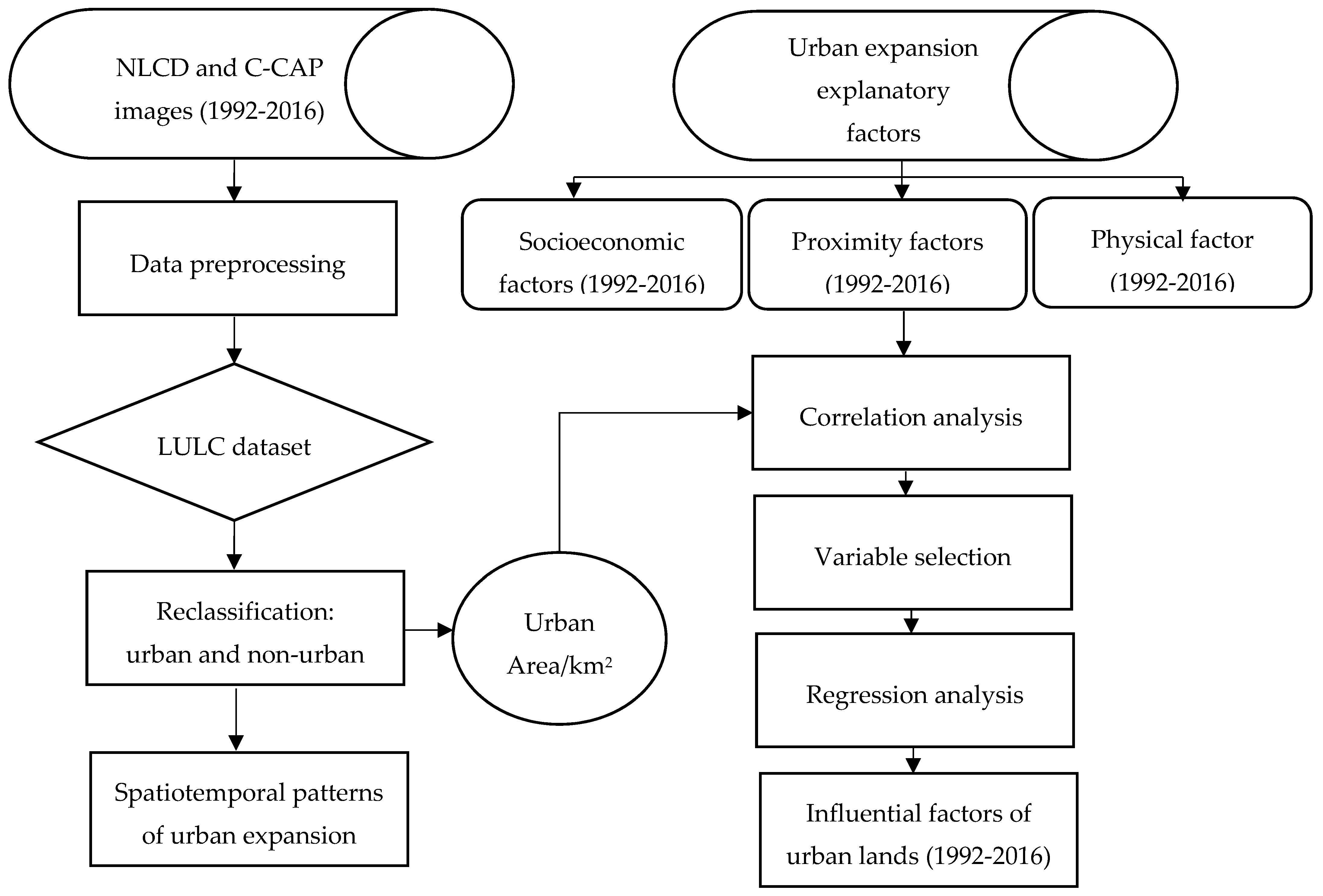
where x’i is the normalized value of the ith cell of variable x, xi is the value of ith cell of variable x, xmax is the maximum value of variable x, and xmin is the minimum value of variable x. After normalization, the value of the dependent and independent variables ranges from 0 to 1. The regression model is acceptable when the p-value is below 0.05 and a high Adjusted R2 value means a better model fit. Figure 2 illustrates the methodology of this study below.

3. Results

3.1. Urban Expansion Rate

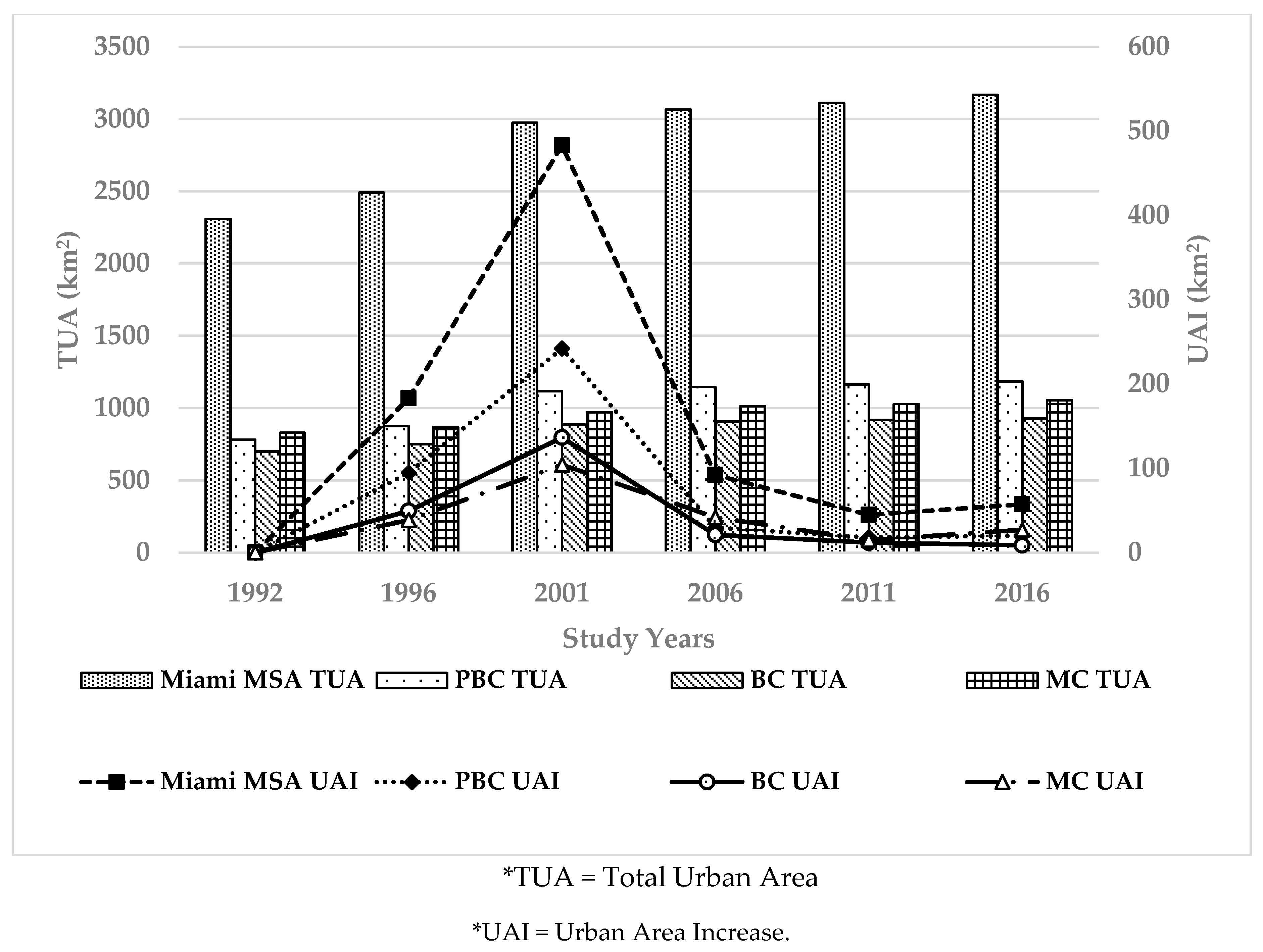
The Miami MSA has gone through a moderate but noticeable urban expansion over the last 25 years (Figure 3 and Appendix A) where the proportion of urban land increased and non-urban land decreased. From the period 1992 to 2016, the urban land increased from 2308.28 km2 to 3167.78 km2 which is 859.5 km2 of newly developed urban land in total in the last 25 years. The AUEa in this period was 34.38 km2 year−1. To get the sense of urban expansion in the study area more locally, we then looked into the urban expansion in the last 25 years in the three counties (Palm Beach, Broward, and Miami-Dade) individually. The urban land in Palm Beach County (PBC) increased substantially where the total urban land in 1992 was 780.01 km2 and it increased to 1183.77 km2 in 2016 with an average annual growth rate of 16.15 km2 year−1. Urban land expanded with an average growth rate of just over 9 km2 year−1 in both Broward County (BC) and Miami-Dade County (MC) (Figure 3).
However, these urban expansions were not the same across different time periods. In Miami MSA, the AUEa was 45.7 km2 year−1 from 1992 to 1996 and 96.57 km2 year−1 between 1996 and 2001. After 2001, there was a sharp decrease in urban land growth in this area. The rate decreased to 18.41 km2 year−1 from 2001 to 2006 and continued to decrease till 2011 when it was found as 8.91 km2 year−1. It then again increased to 11.45 km2 year−1 between the period 2011–2016 (Table 4).
Similarly, PBC experienced rapid urban expansion between the periods 1992–1996 and 1996–2001 where the AUEa were 23.64 and 48.39 km2 year−1. After 2001, it had a steep decrease in AUEa until 2011 when the rate was 3.56 km2 year−1. After 2011, it again had a slight increase with 4.02 km2 year−1. AUEa in MC between 1992 –1996 and 1996 –2001 were the lowest among three counties when the rate was found as 9.63 and 20.82 km2 year−1, respectively. After 2001, it experienced a sharp decrease until 2016. However, between the period 2001–2006 and 2011–2016, MC had the highest AUEa in the tri-county region where the rate was 8.34 and 5.38 km2 year−1, respectively. In BC, AUEa was 12.31 km2 year−1 between 1992–1996 and 27.28 km2 year−1 between 1996–2001. Following the same pattern as other counties, it then continued to decrease till the end when the rate was only 1.72 km2 year−1 in the period 2011–2016 (Table 4). PBC had the highest rate of overall (1992–2016) AUEa (16.15 km2 year−1) among these three counties and MC and BC had almost same overall AUEa (9.08 and 9.04 km2 year−1, respectively).
The overall AUEs in Miami MSA between the period 1992–2016 was found as 1.27%. Again, in the beginning, between 1992–1996, the rate was almost 2%. Then it increased to 3.61% between 1996–2001. After 2001, it experienced a sharp decrease till the end (2011–2016) where the AUEs were below 1% in this area. The AUEs in PBC were almost 3% between 1992–1996 which accounts for the highest rate of standardized annual urban expansion between the three counties in this period. It then increased to 5% between 1996–2001. After 2001, it had a sharp decrease till 2016 where the AUEs were below 1% in all the period making the overall average AUEs in PBC as 1.68%. In BC and MC, the AUEs were 1.71% and 1.14% respectively between the period 1992–1996. It then increased to 3.4% and 2.29% respectively in the following period (1996–2001). After 2001, BC experienced a steep decrease in AUEs as it went below 1% for the rest of the periods. MC also experienced a noticeable decrease in AUEs as it was 0.84% in the period (2001–2006), 0.29% between 2006–2011, and increased to 0.52% again between 2011–2016. Interestingly, both the BC and MC had almost the similar overall average AUEs including 1.13% and just below 1%, respectively, over the last 25 years considering the AUEa in MC was substantially lower than that of BC (Table 4).

3.2. Urban Expansion Types

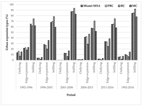
Figure 4 shows the percentages of urban expansion types for the newly developed urban lands in Miami MSA, PBC, BC, and MC area over the five different time periods. Infilling was found as the leading urban expansion type (more than 50%) and outlying as the least dominant expansion type in all the time periods for all the areas. In Miami MSA, the infilling expansion type accounts for 65.06% in 1992–1996. Then it continues to increase till 2006 when the infilling type accounts for over 87% of the total proportion of extension types. During 2006–2011, it decreased to 57.65% and then again increased to 64.42% during 2011–2016 making the overall average of infilling type as 84.4% in Miami MSA. The outlying type in Miami MSA during 1992–1996 was 13.44%. It then started to decrease until 2011 when the proportion of outlying type was below 1%. During 2011–2016, it again increased to 2.14% in this area. The proportion of edge-expansion ranges from 12.53% (2001–2006) to 41.36% (2006–2011) in Miami-MSA.
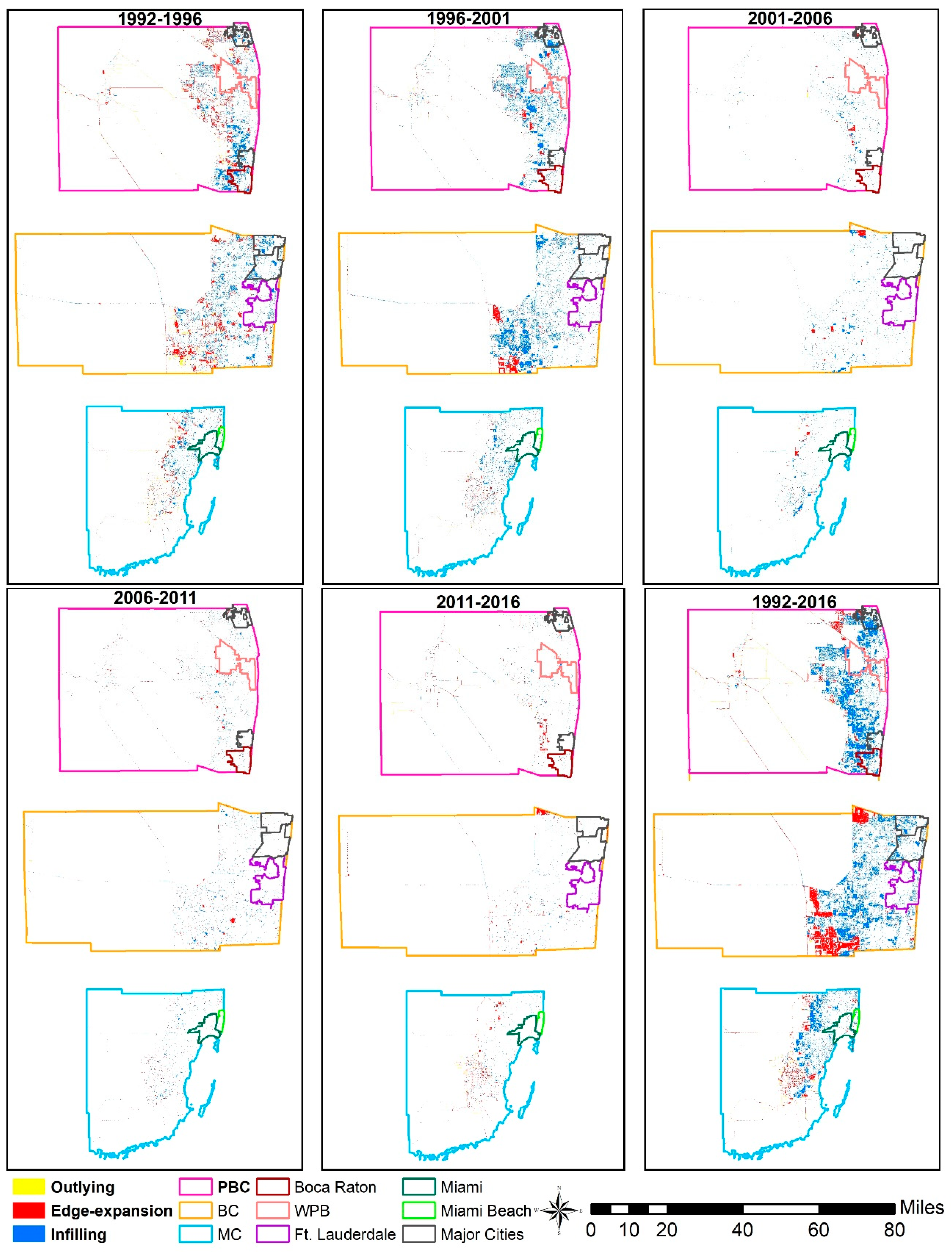
All three counties (PBC, BC, and MC) more or less follow the same trend as the overall study area (Miami MSA) as infilling was the dominant expansion type over all the study periods. Outlying was the least dominant type of expansion in PBC as it was 15.9% during 1992–1996. Then it started to decrease in the following periods until 2006 when it was almost zero (0.13%). During 2006–2011, it increased to almost 1% and then between 2011–2016 it increased to 2.14%. During 1992–1996, the infilling expansion type accounted for 65.06% of the total expansion types. It then increased to 87.34% during 2001–2006. The lowest proportion of infilling type was during 2006–2011 (56.68%). It then again increased to almost 65% during the following period (2011–2016). In BC, the highest proportion of infilling type (93.37%) and the lowest proportion of outlying type (0.06%) was during 2001–2006. Outlying was the highest during 1992–1996 (7.35%) and infilling was the lowest during the period 2006–2011 (70.6%). In MC, infilling was also the highest during 2001–2006 (almost 83%). However, during 2006–2011, edge-expansion was the very dominant type of expansion type as it accounted for almost 47% of the total proportion and infilling was the lowest (51.82%). Edge-expansion was 38.62% during 2011–2016 in MC and outlying was the highest at the beginning (1992–1996) as it accounted for almost 15% of the total proportion.

3.3. Urban Expansion Intensity Index

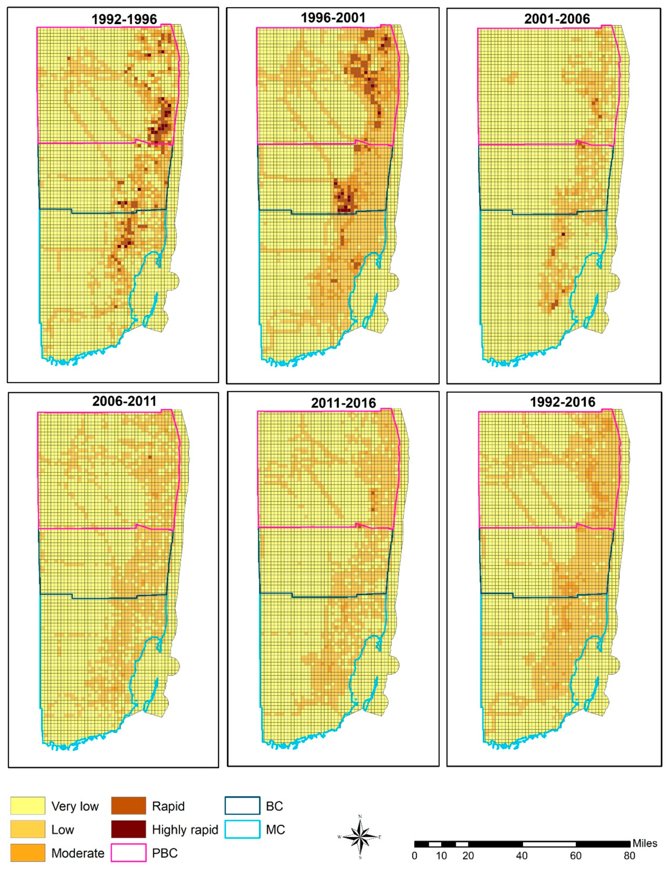
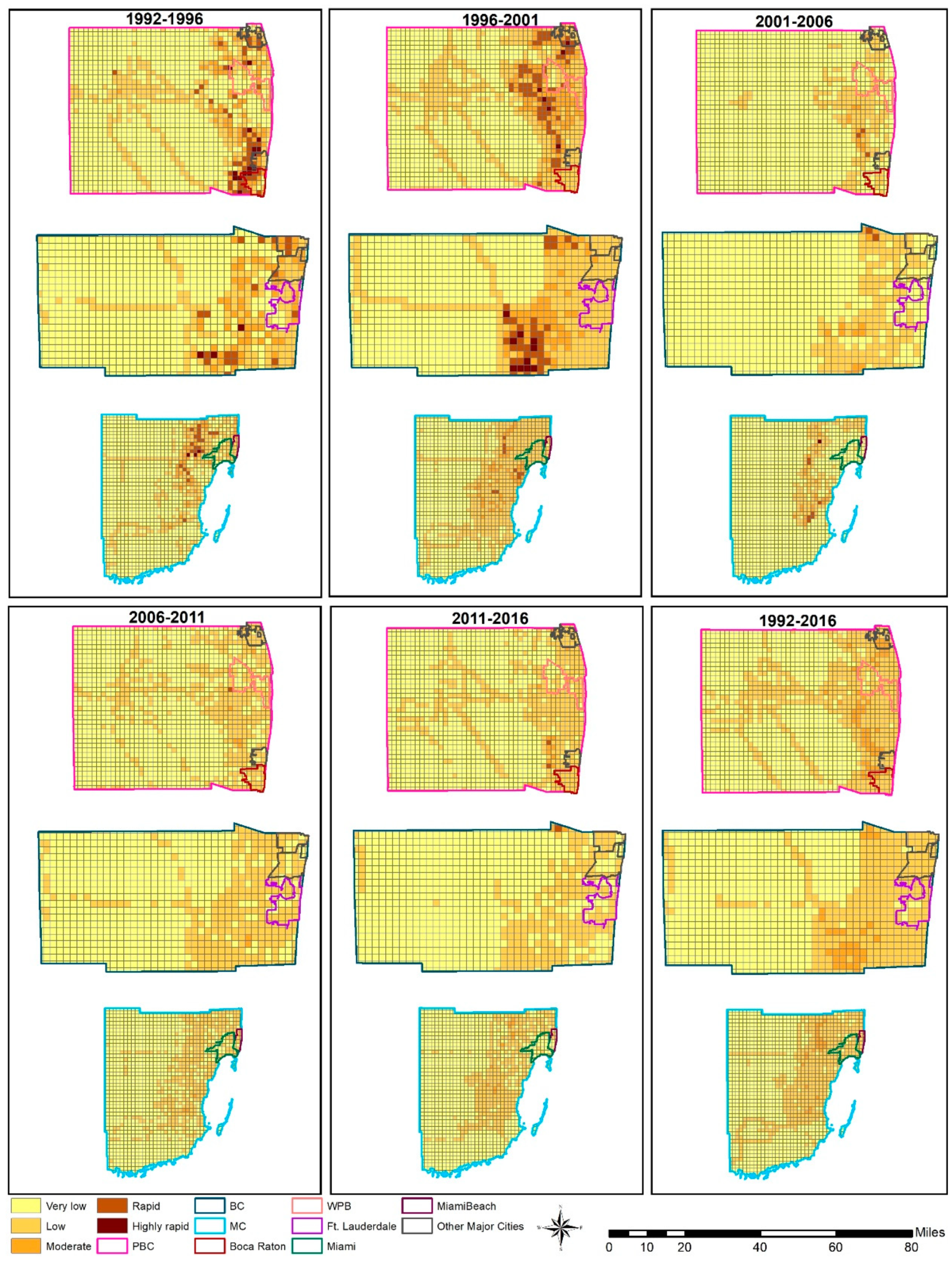
Urban expansion intensity has been examined to evaluate the spatial distribution of urban expansion over the study area from 1992 to 2016 in a five-year interval. To understand the pattern of urban expansion intensity more locally, we overlayed the county boundary over the MSA map (Figure 5) and boundaries of most historical and populous cities over the county map (Figure 6). Figure 5 shows that urban expansion mainly occurred on the east coast of the study area. Most of the rapid and highly rapid urban expansion grids are between 1992–2001 in Miami MSA (Figure 5 and Figure 7). More specifically, rapid and highly rapid expansion grids account for over 3% in the periods 1992–1996 and 1996–2001. After 2001, rapid and highly rapid urban expansion grids decreased significantly.
The proportion of rapid and highly rapid grids in the following periods and there were no rapid and highly rapid expansion grids overall (1992–2016) in this region (Figure 7). Very low and low urban expansion grids account for over 85% of the total proportion over all the study periods in this region. There are some ‘hotspots’ of rapid and highly rapid urban expansion grids during 1992–1996 and 1996–2001 (Figure 5). In PBC, rapid and highly rapid urban expansion grids are clustered together in the south-eastern part of the county which is near the coast during 1992–1996. During 1996–2001, the ‘hotspots’ of rapid and highly rapid urban expansion grids were moved away from the coast and can be seen in the northern part of the county. In BC, rapid and highly rapid expansion grids are dispersed during the period 1992 to 1996. During 1996–2001, there is clearly a cluster of the grids of such kinds at the southern part of the county which is further away from the east coast. In MC, most of the rapid and highly rapid expansion grids are located in the northern part of the county during 1992–1996 and they are away from the coast. During 1996–2001, that cluster is no longer available, and the grids of rapid and highly rapid expansions are rather dispersed. After 2001, the cluster of rapid and highly rapid urban expansion grids started to diminish in this county like the other two counties. However, during 2001–2006, there were still some rapid and highly rapid dispersed grids in this county which completely disappeared after 2006.
Figure 6 shows the spatial pattern of urban expansion intensity at the city level. In PBC, most of the rapid and highly rapid expansion grids are located within or around some major city areas like Boca Raton during 1992–1996. Interestingly, during 1996–2001, most of these grids were shifted away from the major city areas. Since all these major cities are adjacent to the east coast of the study area, it means that most of these grids were shifted away from the beach as well. The same happens in the cities in BC. Although the rapid and highly rapid expansions in this county are dispersed during 1992–1996, it was still within or around the major cities in the county (e.g.,: Fort Lauderdale). However, during 1996–2001, there was a clustered pattern of these grids which was further away from the major cities and the coast. This dispersed pattern of rapid and highly rapid urban expansion grids suggests that high-intensity urban expansion was occurring outside the major city areas in the study area. Cities in the MC follows the same pattern as well. After 2001, rapid and highly rapid urban expansion grids are no longer visible in this region.

3.4. Landscape Metrics

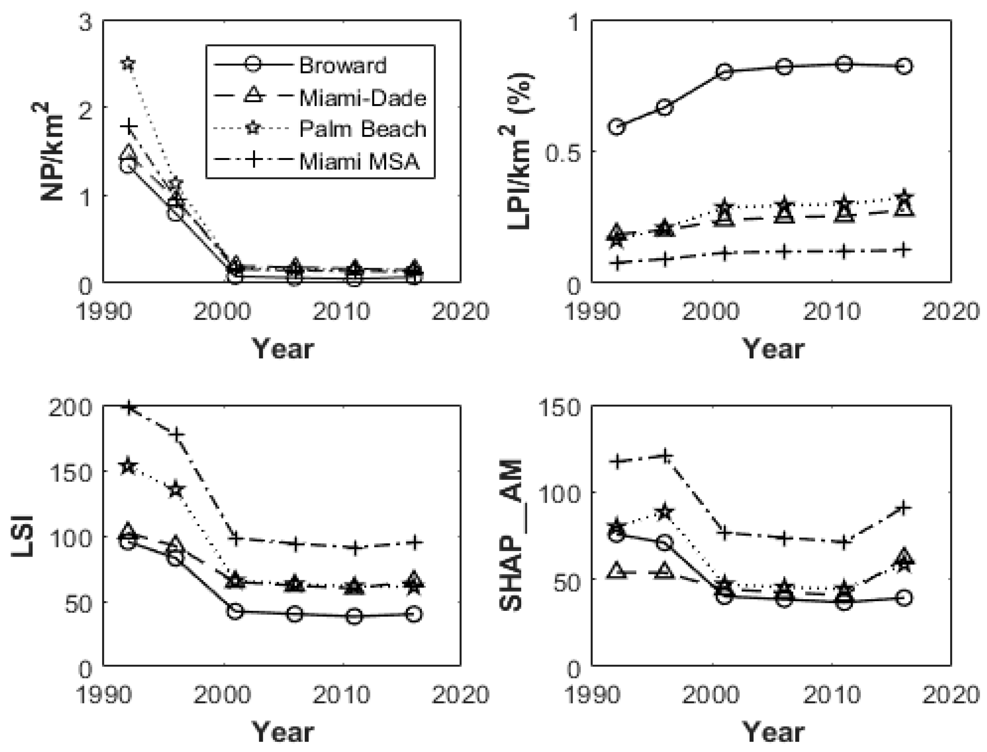
To further examine the patterns of urban expansion in the study area, three class-level metrics including NP, LPI, and SHAP_AM and one landscape-level metric (LSI) are calculated at the MSA and County level (Figure 8). To minimize the size effect, NP and LPI were divided by the respective MSA and County area. NP decreased from 1992 to 2001 and then it was stable for the Miami MSA. The three counties (PBC, BC, and MC) follows the same pattern. However, the highest value of NP was different for the three counties. PBC had the highest value of NP among these three counties followed by MC, and then BC. LPI increased rapidly from 1992 until 2001 in Miami MSA which means rapid urban expansion in this period. After 2001, LPI increased very slowly in this area. Although all the counties followed this pattern more or less exactly, BC among the three counties had the highest percentages of LPI in all the time periods. PBC had the lowest percentage of LPI at the beginning (1992). After 1996, it had higher percentages of LPI than MC. SHAP_AM, which measures the mean shape complexity of discrete patches, decreased from 1996 to 2001 in Miami MSA. After 2001, it was almost stable till 2011. From 2011 to 2016, it increased rapidly (Figure 8). In PBC, it shows a noticeable increase from 1992 to 1996, then decreased rapidly till 2001. During 2001–2011, it was stable and then increased again in the last period (2011–2016). In BC, SHAP_AM decreased right after 1992 till 2011. After 2001, it shows almost a flat line, which means that it was stable till 2016. In MC, it was slowly decreasing from 1996 until 2001. From 2001 to 2011, it was stable and had a rapid increase in the last period (2011–2016).
LSI shows a rapid decreasing pattern from 1992 to 2011 in Miami MSA where LSI decreased in almost half (from almost 200 to 100). After 2001, it was stable till the end (2016) which indicates patch shape was becoming complex. PBC and BC follow the same exact pattern as Miami MSA. In MC, LSI was still decreasing during 1992–2001, but it was rather a slow decrease compared to other two counties. After 2011, it shows a slight increase in LSI also.
The decreasing number of NP throughout the study period suggests that newly developed urban lands became more aggregated after 1992 in Miami MSA and in all three counties. After a sharp decrease until 2001, the rate of decrease in NP slowed down till the end (2016). Unlike NP, LPI increased during the entire study period at all administrative levels (MSA and County) which indicates an increase in urban centers in the study area. The decreasing trend in LSI and SHAP_AM leads to simplified form of urban patches and land areas in the study area.

3.5. Urban Expansion Direction

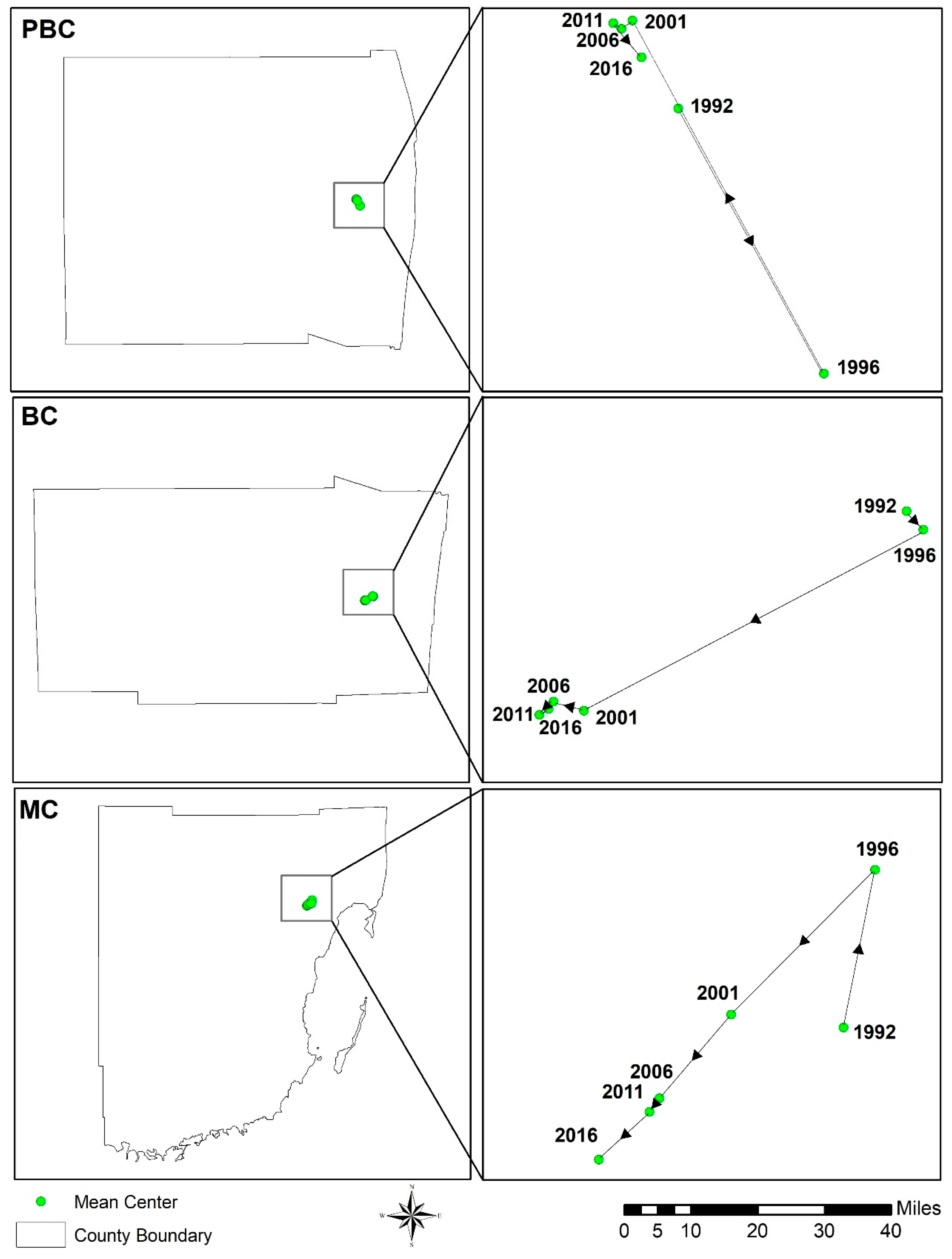
Figure 9 shows the shift in the mean center of the urban areas in Miami MSA from 1992 to 2016. There is a northward shift in the mean center of urban areas from 1992 to 2001. During this period (1992–2001), the mean center first turned towards the east in 1992–1996 and then towards west in 1996–2001. After 2001, the mean center displays a slightly inverse shift from north to south in 2001–2016 while turning towards further west. Although the mean center in the entire study period remained almost stable, there is clearly a westward turn in the mean center in this period. We then further explored the change in mean center of urban areas at the county level. Figure 10 shows the mean center change from 1992–2016 in PBC, BC, and MC. In PBC, the mean center of urban areas shifted towards southeast in 1992–1996. After 1996, there is a significant opposite turn in the mean center in 1996–2001 when it shifted towards a northwest direction. The period 2001–2011 remained steady until 2016 when the mean center in PBC shows a slight turn towards southeast direction. Unlike PBC, BC shows a southwest shift in mean center of urban areas overall (1992–2016). Although after 2001, the mean center remained almost stable in BC while turning towards further west. In MC, urban area means center shifts towards north in 1992–1996. After 1996, it experienced a reverse change towards southwest until 2016.

3.6. Statistical Analyses

The results of the correlation and regression analysis are portrayed in Table 5. Six multiple linear stepwise regression models were built, one for each study year from 1992 to 2016. Each model explained more than half (Adjusted R2 is above 0.5) of the total variation in urban land. The population was found as the variable that explains most of the variance in urban land area in each year except at the end (year 2016). In 2016, variable Distance to Coast was the most significant variable in explaining the total variance. In 1992 and 1996, Distance to Coast entered in the model as the second explanatory variable followed by Distance to Roads. Median Income was not an entry variable in the first two years’ model (1992 and 1996) and last year’s model (2016). From 2001 to 2011, Distance to Coast was the second entry variable in each year’s model followed by Distance to Roads and Median Income, respectively. In 2016, Population was the second entry variable in the model and Distance to Roads was the last to enter the model. Elevation (DEM) did not have any statistically significant strong correlation with urban land and therefore, elevation was not selected as one of the independent factors in the models. Since the land surface is mostly flat in the south Florida region and elevation does not change very frequently, our findings of elevation not having any strong relationship with urban land area are admissible.
In all models, Population, Distance to Coast, and Distance to Roads are accounted for approximately 90% of the total variation of urban land explained. Median Income was not found influential to the variation of urban land areas explained in 1992, 1996, and 2016. For the rest of the years (2001–2011), Median Income had a weak positive correlation with urban land areas and limited influence in explaining the variance in urban land areas. The population had a strong positive correlation with urban land areas and positive model coefficients in all the study areas indicating that higher population increases urban land areas in each of the study periods. Additionally, Distance to Coast and Distance to Roads had strong negative correlations with urban land areas and negative model coefficients in each year indicating that shorter distances from coast and major roads increase urban land areas regardless of the study year. High tolerance value (close to 1) and low VIF values (1<VIF>3) in the correlation matrix in each year’s model suggest that there was a very low degree of multicollinearity among the independent variables.

4. Discussion

4.1. Spatiotemporal Patterns of Urban Expansion

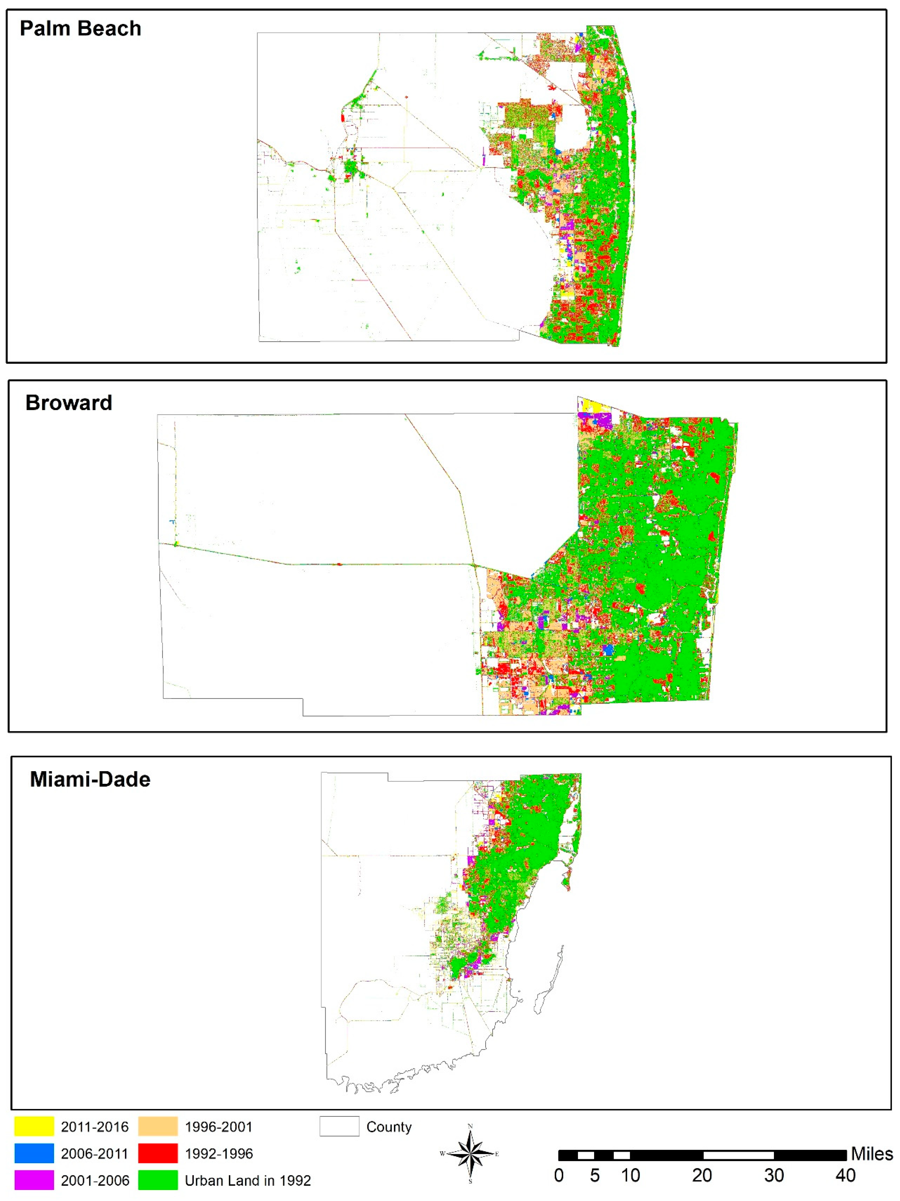
The results portrayed above show the spatiotemporal changes of urban expansion in Miami MSA and the three counties (PBC, BC, and MC) within this metropolitan area (Figure 11) over the last 25 years (1992–2016). The urban land area expanded around 1.37 times in 2016 than the initial land area in 1992 in Miami MSA (Section 3.1). However, urban expansion at the county level was different. Urban land in PBC expanded almost 1.52 times in 2016 than the initial size in 1992. Urban land expansion in BC and MC were comparatively slower than PBC but almost like each other (1.32 and 1.28 respectively) in this period. Urban land expanded rapidly during the period 1992 to 2001 in the Miami MSA and at the county level, especially between 1996–2001 when urban land expansion almost doubled than the previous study year (1992–1996), but decreased dramatically afterward (2001–2016) in this region (Figure 3). In late 1980s, this region experienced a rapid population growth due to industrial and economic development, which generated lavish job opportunities and attracted migrants from other parts of the country. These intra-national migrants along with booming tourism sector resulted thriving housing sector, and hotel and recreational facilities development. All these factors contributed to rapid urbanization in 1990s in the study area. However, population growth started to decline considerably since the beginning of 2000s. The population growth rate was found 23.5% between 1990 and 2000 in this region. However, between 2000 and 2010, this population growth rate declined to 11.4% in this area. Although the rate of population growth slowed down after 2000, it is estimated that population will still continue to increase in this region and therefore urban land expansion will further increase considerably after 2016 in the study area.
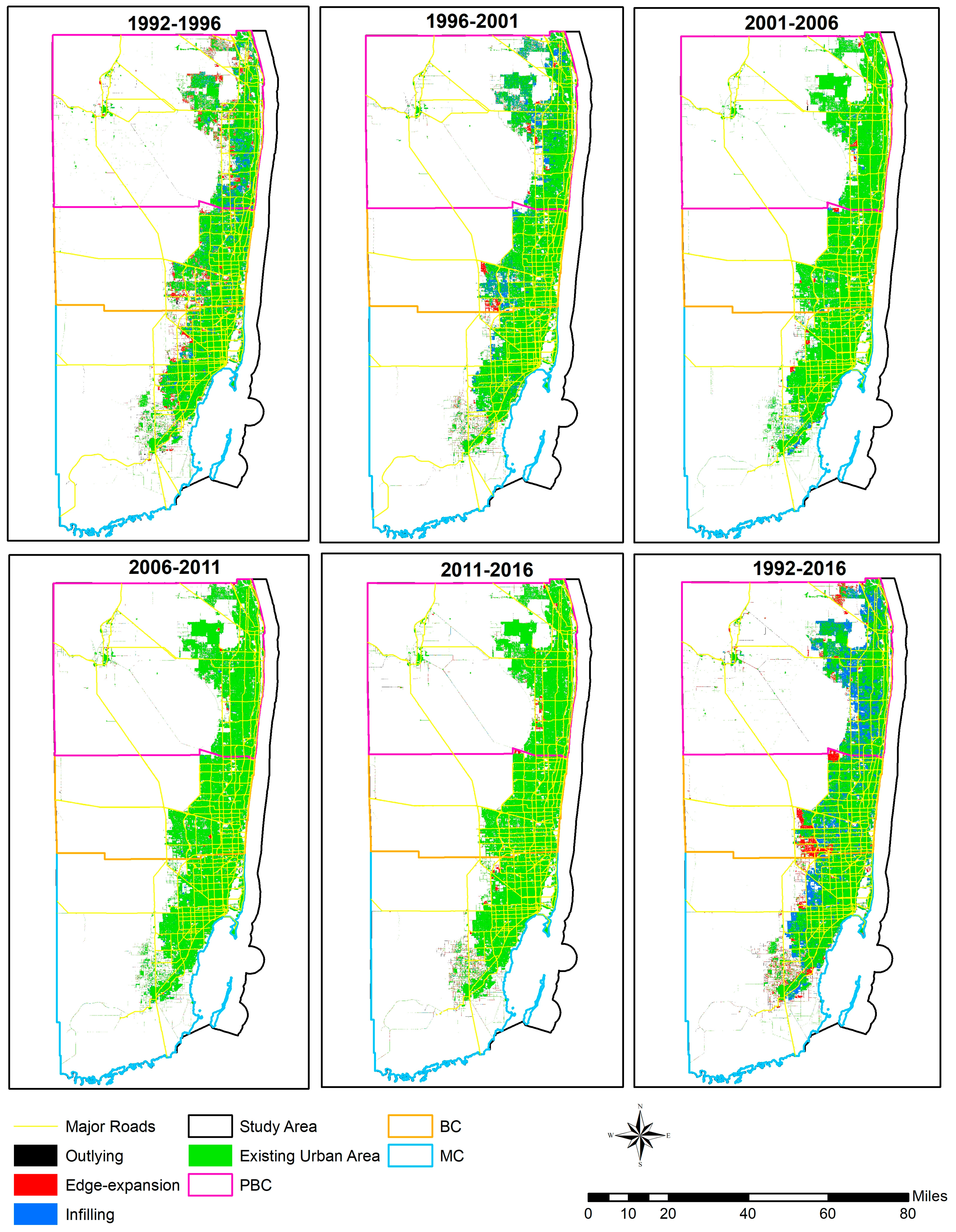
The types of urban expansion varied between the study periods in the study area (Section 3.2). While the urban expansion was isolated at the beginning (1992–1996), it became more aggregated and showed clusters of urban lands in the following periods which might be related to the formation of infilling and edge-expansion types of urban growth [26,30]. This compactness in urban expansion continued to increase with the increase of infilling expansion type in the Miami MSA and the three counties (Figure 12 and Figure 13). Interestingly, most of these urban expansions occurred outside of the most prominent and historic city boundaries in the study area (Figure 13). Additionally, major roads of the ending year in each study period (e.g., 2016 roads for period 2011–2016) were used to see if the outlying expansion types were influenced/guided by roads (Figure 12). Figure 12 shows that the outlying expansion types were rather dispersed/scattered in pattern than following or guided by the road networks in each year in Miami MSA. Similarly, most of the rapid and highly rapid urban expansion intensity grids were found between the years 1992 and 2001 (Section 3.3). After 2001, rapid and highly rapid expansion grids decreased dramatically as urban expansion rate slowed down substantially after 2001. Additionally, most of the moderate-highly rapid expansion grids were outside of the major city boundaries which are in line with above results. Urban expansion in the developed region causes a few problems including extreme land price increase, environmental pollution, and rapid rising of living costs which make people move outside of the city area to the suburban region [35] and eventually construct new urban cities/cores. Results from the landscape metrics are consistent with these findings (Section 3.4). The decreasing trend of NP, LSI, and SHAP_AM indicates that urban lands are becoming more aggregated and less complex than the past with their expansion as evidenced in previous studies [26] while continuous increase in LSI represents an increase in the urban center. This also suggests that many non-urban patches initially located in the urban areas might have been transformed into urban patches which are also evident in previous studies [57]. Additionally, a decrease in NP and increase in LPI is an indication of infilling expansion type along with aggregated development [57]. Since infilling expansion type is dominant during the whole study period, along with a continuous decreasing trend in NP and increasing trend in LPI, our results of a more aggregated form of urban expansion process with simplified form of urban lands are reasonable.
Furthermore, urban land expansions are moving away from the east coast of the study area and directed towards the west (Section 3.5), which is evident in mean center of urban lands from 1992–2016 (Figure 9 and Figure 10). Although very slowly, this westward turn of mean center of Miami MSA and the three counties proves our previous hypothesis that urban lands are expanding towards suburb region (west side) of the study area since the east part of the study area are already developed. Being very near to the coastline which poses high recreational value and better transportation access, demands on land parcels are extremely high on the east side of the study region and eventually the land prices are skyrocketing. All these reasons might be responsible for the urban lands expanding toward west part of the study area and away from the east coast. With the increasing conversion of nonurban lands to urban land, it will be extremely difficult to protect the environment and biodiversity in the coming years [14,15,60].

4.2. Major Explanatory Factors of Urban Expansion

Four of the five selected variables of urban expansion had strongly statistically significant relationships with the urban land areas during the study period (Section 3.6). Elevation, which was preliminarily selected as a physical factor of urban land expansion did not have significant relationship with urban land area in any study year (1992–2016). Since the land surface is almost flat throughout the study region and there is not much change in elevation from mean sea level in this region, this result was not surprising. The population had a very strong positive relationship with urban land in all six study years since it is found as one of the most important socio-economic factors driving urban expansion in previous studies [36,46]. Surprisingly, median household income did not have a very strong relationship with urban land expansion except in 2011 and did not even enter the regression models in year 1992, 1996, and 2016. This suggests that median income had very little to do in guiding urban expansion in this region. Unlike developing countries, people here in the US with high median household income tend to live outside of the urban core which might cause a weak statistical relationship with urban lands and median income. However, previous studies found other factors like gross domestic product (GDP), secondary and tertiary industry product, gross output of construction industry as factors of economic development that influence urban expansion [36,46]. However, based on available data and spatial scale of the study area, median household income was selected as one of the socioeconomic factors that influence urban expansion in this study. Distance to Coast and Distance to Roads both had strong negative relationships with urban land in all the years which suggest that urban land area expanded within proximity to major roads and coastal boundary.
Population and Distance to Coast had the strongest relationship with urban land in all the six models followed by Distance to Roads and Median Income except in 1992. In 1992, the population was the least strong variable. This is due to the increase in population in this area. According to US Census Bureau, the total population in Miami MSA was about 4,056,100 in 1990. In 2000, total population increased to 5,007,564 which is about 23.5% increase from 1990. In 2010, total population increased to 5,564,635 which is about 11.1% increase from 2000. In 2018, it is estimated that the total population is 6,198,782 which is 11.4% increase from 2010 in this region.
In previous studies, factors of urban expansion were analyzed either very briefly [61,62] or using only socioeconomic factors [36]. In this research, we quantified the influence of socioeconomic, proximity, and physical factors on urban land expansion. However, these factors explained over 50% of the variation in urban land during the study period (1992–2016) and inclusion of other factors like urban planning and zoning, policies, hydrological factors, neighborhood impacts, etc., might improve the results.

4.3. Limitations of the Study and Future Work

To retrieve information about urban land and urban expansion at a finer scale, high spatial resolution imagery like QuickBird and Lidar could be used in the future. Due to the unavailability of those high spatial resolution imageries for the entire study year (1992–2016) in our study area, we used moderate resolution (30 m) land cover maps in this study. This research is limited to the horizontal expansion of urban lands only. However, previous studies found that urban expansion is not necessarily limited to horizontal dimension and urban areas could also be expanded vertically [63,64]. Investigating the vertical expansion of urban areas in the study area could help understand the urban growth dynamics more profoundly in future. To understand the effects of urban expansion on non-urban lands, analyzing the relationship between urban expansion and the loss of agriculture, protected and reserved areas would be useful for this region. Since the physical factor used in this research does not have any statistically significant relationship with urban land area, other physical factors like soil characteristics, flood risk zones, physical features like schools and entertainment facilities, etc., could be used in future for a comprehensive analysis of influential factors of urban expansion in the study area. Besides, other factors of urban expansion like hydrological factors, policy, and building codes, development control zones, etc. should be used in explanatory factor analysis in future. Additionally, since the study area region has always been a target of hurricanes over the past few decades, analyzing the impact of hurricane damages on urban land expansion in this area could be advantageous.

5. Conclusions

Urban expansion is one of the most irretrievable land transformation processes in the world and poses major impacts on the environment and challenges for the entire world at global, regional, and local scale. There is still a lack of research that focuses on urban expansion process at local scale in the US. Being a developed country, less attention has been paid on the dynamics of urban expansion in this region than necessary and timely monitoring and evaluation of urban land expansion is extremely important.
In this study, we used NLCD data and C-CAP data combined with urban growth type and landscape metrics analysis to quantify the dynamics of the spatiotemporal pattern of urban expansion in the moderately developed Miami MSA. We then further extended our analysis to examine the spatiotemporal patterns of urban growth at the county level and compared the results between the three counties (PBC, BC, and MC) that are located within the MSA area. More specifically, we analyzed and compared the spatial and temporal distribution of urban expansion rate, pattern, expansion types, urban expansion intensity, and landscape metrics. Results suggest that this region experienced a moderate but noticeable urban expansion over the last 25 years. Urban expansion in this region can be divided into two phases: pre-2001 phase when urban expansion rate was very rapid in this MSA and post-2001 phase when urban expansion rate was moderate/slow. Urban expansion at the county level was almost the same as the MSA where the overall annual urban expansion rate in PBC was the highest (16.15 km2 year−1) followed by BC and MC (9.08 and 9.04 km2 year−1, respectively). The standardized annual urban growth rate for PBC, BC, and MC are 1.68%, 1.13%, and 0.97%, respectively, which suggests a moderate urban expansion overall in these counties.
Similarly, infilling was the dominant expansion type in all the study periods in the MSA and in all three counties. Additionally, they all followed the same pattern of decreasing amount of NP and LSI from the beginning of the study period (1992) which suggests that as the urban land expanded and time progressed in this region, they became more aggregated and simplified. Another interesting finding from the analysis was that the newly developed urban lands were generated away from the east coast in this region over the entire study period which was further corroborated by mean center analysis.
As per the cities were concerned, it was evident that the newly developed urban lands were moving away from the major historical and prominent cities in this region. As urban growth creates pressure on the existing population and increases the cost of living and environmental pollution, people might have forced to move away from the city areas to sub-urban areas and eventually created new ‘urban cores’. Statistical analysis of the major explanatory factors of urban expansion reveals that Population and Distance to Coast had strongest relationships with urban lands where the former had a positive relationship and latter had a negative relationship. Distance to Roads was another variable that had a strong relationship with urban lands followed by Median Household Income in this region. With continuous population growth and economic development, dealing with urban expansion and environment and biodiversity protection in this region would be perplexing in the coming years. Future research should emphasize the improvement of the spatial and spectral resolution of remote sensing data in order to more accurately portray the urban expansion patterns and should include additional factors of urban expansion including that are used in this research to explain the urban expansion characteristics comprehensively. Finally, the methods and techniques utilized in this research could be applied in future studies focusing on the urban expansion patterns in other metropolitan areas.

Author Contributions

Conceptualization, W.L.; Formal analysis, S.A.A.R. and W.L.; Funding acquisition, W.L.; Methodology, S.A.A.R. and W.L.; Writing—original draft, S.A.A.R.; Writing—review & editing, W.L.

Funding

The APC was funded by Florida Atlantic University College of Science seed funding.

Acknowledgments

We would like to thank the five anonymous reviewers and editors for providing valuable comments and suggestions which helped improve the manuscript greatly.

Conflicts of Interest

The authors declare no conflict of interest. The funders had no role in the design of the study; in the collection, analyses, or interpretation of data; in the writing of the manuscript, or in the decision to publish the results.

Appendix A

Table A1. Changes of Urban Land Covers in last 25 years (in km2) in Miami MSA and three counties.
Urban AreaNon-Urban Area
199219962001200620112016199219962001200620112016
Miami-MSA2308.282491.092973.933065.993110.553167.7811848.9411666.1311183.2911091.2311046.6710989.97
PBC780.01874.581116.521145.851163.671183.774982.094887.524645.584616.254598.434578.33
BC699.60748.83885.22906.26917.99926.62470.232421.02284.612263.572251.842243.23
MC828.67867.19971.31013.01027.81054.694396.624358.14253.994212.294197.494170.6

References

  1. United Nations. World Urbanization Prospects, the 2018 Revision; United Nations: New York, NY, USA, 2018; Available online: http://esa.un.org/unpd/wup/index.htm 2018 (accessed on 13 July 2019).
  2. Neumann, B.; Vafeidis, A.T.; Zimmermann, J.; Nicholls, R.J. Future Coastal Population Growth and Exposure to Sea-Level Rise and Coastal Flooding—A Global Assessment. PLoS ONE 2015, 10, e0118571. [Google Scholar] [CrossRef] [PubMed]
  3. Zhao, S.; Zhou, D.; Zhu, C.; Qu, W.; Zhao, J.; Sun, Y.; Huang, D.; Wu, W.; Liu, S. Rates and patterns of urban expansion in China’s 32 major cities over the past three decades. Landsc. Ecol. 2015, 30, 1541–1559. [Google Scholar] [CrossRef]
  4. Zhao, S.; Da, L.; Tang, Z.; Fang, H.; Song, K.; Fang, J. Ecological consequences of rapid urban expansion: Shanghai, China. Front. Ecol. Environ. 2006, 4, 341–346. [Google Scholar] [CrossRef]
  5. Shi, Y.; Li, S. Research on Rational Urban Growth and Land-Use Issues. J. Urban Plan. Dev. 2007, 133, 91–94. [Google Scholar] [CrossRef]
  6. Grimm, N.B.; Faeth, S.H.; Golubiewski, N.E.; Redman, C.L.; Wu, J.; Bai, X.; Briggs, J.M.; Grimm, N. Global Change and the Ecology of Cities. Science 2008, 319, 756–760. [Google Scholar] [CrossRef] [Green Version]
  7. Jenerette, G.D.; Potere, D. Global analysis and simulation of land-use change associated with urbanization. Landsc. Ecol. 2010, 25, 657–670. [Google Scholar] [CrossRef]
  8. Zheng, Z.; Bohong, Z. Study on Spatial Structure of Yangtze River Delta Urban Agglomeration and Its Effects on Urban and Rural Regions. J. Urban Plan. Dev. 2012, 138, 78–89. [Google Scholar] [CrossRef]
  9. Tan, M.; Li, X.; Xie, H.; Lu, C. Urban land expansion and arable land loss in China—A case study of Beijing–Tianjin–Hebei region. Land Use Policy 2005, 22, 187–196. [Google Scholar] [CrossRef]
  10. Radeloff, V.C.; Stewart, S.I.; Hawbaker, T.J.; Todd, J.; Gimmi, U.; Pidgeon, A.M.; Flather, C.H.; Hammer, R.B.; Helmers, D.P. Housing growth in and near United States protected areas limits their conservation value. Proc. Natl. Acad. Sci. USA 2010, 107, 940–945. [Google Scholar] [CrossRef]
  11. Folke, C.; Jansson, A.; Larsson, J.; Costanza, R. Ecosystem appropriation by cities. Ambio 1997, 26, 167–172. [Google Scholar]
  12. Jenerette, G.D.; Wu, J. Analysis and simulation of land-use change in the central Arizona—Phoenix region, USA. Landsc. Ecol. 2001, 16, 611–626. [Google Scholar] [CrossRef]
  13. Wu, J.; Jenerette, G.D.; Buyantuyev, A.; Redman, C.L. Quantifying spatiotemporal patterns of urbanization: The case of the two fastest growing metropolitan regions in the United States. Ecol. Complex. 2011, 8, 1–8. [Google Scholar] [CrossRef]
  14. Seto, K.C.; Gu¨neralp, B.; Hutyra, L.R. Global forecasts of urban expansion to 2030 and direct impacts on biodiversity and carbon pools. Proc. Natl. Acad. Sci. USA 2012, 109, 16083–16088. [Google Scholar] [CrossRef] [PubMed] [Green Version]
  15. He, C.; Liu, Z.; Tian, J.; Ma, Q. Urban expansion dynamics and natural habitat loss in China: A multiscale landscape perspective. Glob. Chang. Boil. 2014, 20, 2886–2902. [Google Scholar] [CrossRef] [PubMed]
  16. Shao, M.; Tang, X.; Zhang, Y.; Li, W. City clusters in China: Air and surface water pollution. Front. Ecol. Environ. 2006, 4, 353–361. [Google Scholar] [CrossRef]
  17. Chen, Y.; Zhang, Z.; Du, S.Q.; Shi, P.J.; Tao, F.L.; Doyle, M. Water quality changes in the world’s first special economic zone, Shenzhen, China. Water Resour. Res. 2011, 47. [Google Scholar] [CrossRef]
  18. Baker, L.A.; Hope, D.; Xu, Y.; Edmonds, J.; Lauver, L. Nitrogen Balance for the Central Arizona-Phoenix (CAP) Ecosystem. Ecosystems 2001, 4, 582–602. [Google Scholar] [CrossRef]
  19. Kaye, J.P.; Groffman, P.M.; Grimm, N.B.; Baker, L.A.; Pouyat, R.V. A distinct urban biogeochemistry? Trends Ecol. Evol. 2006, 21, 192–199. [Google Scholar] [CrossRef]
  20. Trusilova, K.; Jung, M.; Churkina, G.; Karstens, U.; Heimann, M.; Claussen, M. Urbanization Impacts on the Climate in Europe: Numerical Experiments by the PSU–NCAR Mesoscale Model (MM5). J. Appl. Meteorol. Clim. 2008, 47, 1442–1455. [Google Scholar] [CrossRef]
  21. Yang, X.; Hou, Y.; Chen, B. Observed surface warming induced by urbanization in east China. J. Geophys. Res. Atoms. 2011, 116, 116. [Google Scholar] [CrossRef]
  22. Walker, R. Urban sprawl and natural areas encroachment: Linking land cover change and economic development in the Florida Everglades. Ecol. Econ. 2001, 37, 357–369. [Google Scholar] [CrossRef]
  23. Jensen, J.R.; Cowen, D.C. Remote sensing of urban/suburban infrastructure and socio-economic attributes. Photogramm. Eng. Remote Sens. 1999, 65, 611–622. [Google Scholar]
  24. Herold, M.; Goldstein, N.C.; Clarke, K.C. The spatiotemporal form of urban growth: Measurement, analysis and modeling. Remote Sens. Environ. 2003, 86, 286–302. [Google Scholar] [CrossRef]
  25. Michishita, R.; Jiang, Z.; Xu, B. Monitoring two decades of urbanization in the Poyang Lake area, China through spectral unmixing. Remote Sens. Environ. 2012, 117, 3–18. [Google Scholar] [CrossRef]
  26. Sun, Y.; Zhao, S.; Qu, W. Quantifying spatiotemporal patterns of urban expansion in three capital cities in Northeast China over the past three decades using satellite data sets. Environ. Earth Sci. 2015, 73, 7221–7235. [Google Scholar] [CrossRef]
  27. Turner, M.G.; Gardner, R.H. Quantitative Methods in Landscape Ecology; Springer: New York, NY, USA, 1991. [Google Scholar]
  28. McGarigal, K.; Marks, B.J. FRAGSTATS: Spatial Pattern Analysis Program for Quantifying Landscape Structure; USDA Forest Service: Washington, DC, USA, 1995; Volume 351. [Google Scholar]
  29. Sudhira, H.; Ramachandra, T.; Jagadish, K. Urban sprawl: Metrics, dynamics and modelling using GIS. Int. J. Appl. Earth Obs. Geoinf. 2004, 5, 29–39. [Google Scholar] [CrossRef]
  30. Xu, C.; Liu, M.; Zhang, C.; An, S.; Yu, W.; Chen, J.M. The spatiotemporal dynamics of rapid urban growth in the Nanjing metropolitan region of China. Landsc. Ecol. 2007, 22, 925–937. [Google Scholar] [CrossRef]
  31. Zhao, J.; Zhu, C.; Zhao, S. Comparing the Spatiotemporal Dynamics of Urbanization in Moderately Developed Chinese Cities over the Past Three Decades: Case of Nanjing and Xi’an. J. Urban Plan. Dev. 2015, 141, 5014029. [Google Scholar] [CrossRef]
  32. Zhao, S.; Zhou, D.; Zhu, C.; Sun, Y.; Wu, W.; Liu, S. Spatial and Temporal Dimensions of Urban Expansion in China. Environ. Sci. Technol. 2015, 49, 9600–9609. [Google Scholar] [CrossRef]
  33. Ramachandra, T.V.; Aithal, B.H.; Sanna, D.D. Insights to urban dynamics through landscape spatial pattern analysis. Int. J. Appl. Earth Obs. Geoinf. 2012, 18, 329–343. [Google Scholar]
  34. Li, Q.; Lu, L.; Weng, Q.; Xie, Y.; Guo, H. Monitoring Urban Dynamics in the Southeast U.S.A. Using Time-Series DMSP/OLS Nightlight Imagery. Remote Sens. 2016, 8, 578. [Google Scholar] [CrossRef]
  35. Shi, G.; Jiang, N.; Li, Y.; He, B. Analysis of the Dynamic Urban Expansion Based on Multi-Sourced Data from 1998 to 2013: A Case Study of Jiangsu Province. Sustainability 2018, 10, 3467. [Google Scholar] [CrossRef]
  36. Chen, L.; Ren, C.; Zhang, B.; Wang, Z.; Liu, M. Quantifying Urban Land Sprawl and its Driving Forces in Northeast China from 1990 to 2015. Sustainability 2018, 10, 188. [Google Scholar] [CrossRef]
  37. Yu, W.; Zhou, W. The Spatiotemporal Pattern of Urban Expansion in China: A Comparison Study of Three Urban Megaregions. Remote Sens. 2017, 9, 45. [Google Scholar] [CrossRef]
  38. Hu, Y.; Jia, G.; Pohl, C.; Feng, Q.; He, Y.; Gao, H.; Xu, R.; Van Genderen, J.; Feng, J. Improved monitoring of urbanization processes in China for regional climate impact assessment. Environ. Earth Sci. 2015, 73, 8387–8404. [Google Scholar] [CrossRef]
  39. Yang, Y.Y.; Zhang, S.W.; Yang, J.C.; Xing, X.S.; Wang, D.Y. Using a cellular automata-markov model to reconstruct spatial land-use patterns in Zhenlai County, Northeast China. Energies 2015, 8, 3882–3902. [Google Scholar] [CrossRef]
  40. Li, X.M.; Zhou, W.Q.; Ouyang, Z.Y. Forty years of urban expansion in Beijing: What is the relative importance of physical, socioeconomic, and neighborhood factors? Appl. Geogr. 2013, 38, 1–10. [Google Scholar] [CrossRef]
  41. Tian, G.; Qiao, Z.; Zhang, Y. The investigation of relationship between rural settlement density, size, spatial distribution and its geophysical parameters of China using Landsat TM images. Ecol. Model. 2012, 231, 25–36. [Google Scholar] [CrossRef]
  42. Luo, J.; Wei, Y.D. Modeling spatial variations of urban growth patterns in Chinese cities: The case of Nanjing. Landsc. Urban Plan. 2009, 91, 51–64. [Google Scholar] [CrossRef]
  43. Aspinall, R. Modelling land use change with generalized linear models—A multi-model analysis of change between 1860 and 2000 in Gallatin Valley, Montana. J. Environ. Manag. 2004, 72, 91–103. [Google Scholar] [CrossRef]
  44. Ye, Y.; Zhang, H.; Liu, K.; Wu, Q. Research on the influence of site factors on the expansion of construction land in the Pearl River Delta, China: By using GIS and remote sensing. Int. J. Appl. Earth Obs. Geoinf. 2013, 21, 366–373. [Google Scholar] [CrossRef]
  45. Vermeiren, K.; Van Rompaey, A.; Loopmans, M.; Serwajja, E.; Mukwaya, P. Urban growth of Kampala, Uganda: Pattern analysis and scenario development. Landsc. Urban Plan. 2012, 106, 199–206. [Google Scholar] [CrossRef]
  46. Li, G.; Sun, S.; Fang, C. The varying driving forces of urban expansion in China: Insights from a spatial-temporal analysis. Landsc. Urban Plan. 2018, 174, 63–77. [Google Scholar] [CrossRef]
  47. Vogelmann, J.E.; Howard, S.M.; Yang, L.; Larson, C.R.; Wylie, B.K.; Van Driel, N. Completion of the 1990s National Land Cover Data Set for the Conterminous United States from Landsat Thematic Mapper data and ancillary data sources. Photogramm. Eng. Remote Sens. 2001, 67, 650–662. [Google Scholar]
  48. Homer, C.; Dewitz, J.; Fry, J.; Coan, M.; Hossain, N.; Larson, C.; Herold, N.; McKerrow, A.; Van Driel, J.N.; Wickham, J.D. Completion of the 2001 National Land Cover Database for the conterminous United States. Photogramm. Eng. Remote Sens. 2007, 73, 337–341. [Google Scholar]
  49. Mitsova, D.; Shuster, W.; Wang, X. A cellular automata model of land cover change to integrate urban growth with open space conservation. Landsc. Urban Plan. 2011, 99, 141–153. [Google Scholar] [CrossRef]
  50. Yang, L.; Jin, S.; Danielson, P.; Homer, C.; Gass, L.; Bender, S.M.; Case, A.; Costello, C.; Dewitz, J.; Fry, J.; et al. A new generation of the United States National Land Cover Database: Requirements, research priorities, design, and implementation strategies. ISPRS J. Photogramm. Remote Sens. 2018, 146, 108–123. [Google Scholar] [CrossRef]
  51. Wickham, J.; Stehman, S.V.; Gass, L.; Dewitz, J.A.; Sorenson, D.G.; Granneman, B.J.; Poss, R.V.; Baer, L.A. Thematic accuracy assessment of the 2011 National Land Cover Database (NLCD). Remote Sens. Environ. 2017, 191, 328–341. [Google Scholar] [CrossRef] [Green Version]
  52. Wickham, J.; Stehman, S.V.; Gass, L.; Dewitz, J.; Fry, J.A.; Wade, T.G. Accuracy assessment of NLCD 2006 land cover and impervious surface. Remote Sens. Environ. 2013, 130, 294–304. [Google Scholar] [CrossRef]
  53. Wickham, J.; Stehman, S.; Fry, J.; Smith, J.; Homer, C. Thematic accuracy of the NLCD 2001 land cover for the conterminous United States. Remote Sens. Environ. 2010, 114, 1286–1296. [Google Scholar] [CrossRef]
  54. Stehman, S.V.; Wickham, J.D.; Smith, J.H.; Yang, L. Thematic accuracy of the 1992 National Land Cover Data (NLCD) for the eastern United States: Statistical methodology and regional results. Remote Sens. Environ. 2003, 86, 500–516. [Google Scholar] [CrossRef]
  55. Coastal Change Analysis Program (C-CAP) Regional Land Cover. Available online: https://coast.noaa.gov/data/digitalcoast/pdf/ccap-faq-regional.pdf (accessed on 13 October 2019).
  56. Manson, S.; Schroeder, J.; Van Riper, D.; Ruggles, S. IPUMS National Historical Geographic Information System: Version 14.0 [Database]; IPUMS: Minneapolis, MN, USA, 2019. [Google Scholar] [CrossRef]
  57. Fang, C.; Li, G.; Wang, S. Changing and Differentiated Urban Landscape in China: Spatiotemporal Patterns and Driving Forces. Environ. Sci. Technol. 2016, 50, 2217–2227. [Google Scholar] [CrossRef] [PubMed]
  58. Hair, J.F., Jr.; Black, W.C.; Babin, B.J.; Anderson, R.E. Multivariate Data Analysis, 7th ed.; Pearson: New York, NY, USA, 2010; pp. 151–230. [Google Scholar]
  59. Hossain, M.K.; Meng, Q. A thematic mapping method to assess and analyze potential urban hazards and risks caused by flooding. Comput. Environ. Urban Syst. 2020, 79, 101417. [Google Scholar] [CrossRef]
  60. Güneralp, B.; Seto, K.C. Futures of global urban expansion: Uncertainties and implications for biodiversity conservation. Environ. Res. Lett. 2013, 8, 014025. [Google Scholar] [CrossRef]
  61. Li, L.; Lu, D.; Kuang, W. Examining Urban Impervious Surface Distribution and Its Dynamic Change in Hangzhou Metropolis. Remote Sens. 2016, 8, 265. [Google Scholar] [CrossRef]
  62. Dou, Y.; Liu, Z.; He, C.; Yue, H. Urban Land Extraction Using VIIRS Nighttime Light Data: An Evaluation of Three Popular Methods. Remote Sens. 2017, 9, 175. [Google Scholar] [CrossRef]
  63. Zhang, W.; Li, W.; Zhang, C.; Ouimet, W.B. Detecting horizontal and vertical urban growth from medium resolution imagery and its relationships with major socioeconomic factors. Int. J. Remote Sens. 2017, 38, 3704–3734. [Google Scholar] [CrossRef]
  64. Handayani, H.H.; Murayama, Y.; Ranagalage, M.; Liu, F.; Dissanayake, D. Geospatial Analysis of Horizontal and Vertical Urban Expansion Using Multi-Spatial Resolution Data: A Case Study of Surabaya, Indonesia. Remote Sens. 2018, 10, 1599. [Google Scholar] [CrossRef]
Figure 1. Location of the Florida Metropolitan Statistical Area (Miami MSA), three counties, major cities, along with coastline in 2013 and major roads in 1990 within the study area.
Remotesensing 11 02493 g001
Figure 2. Methodological flowchart of the study.
Remotesensing 11 02493 g002
Figure 3. Urban Area Expansion (in km2) in the Study Area over Different Time Periods.
Remotesensing 11 02493 g003
Figure 4. Proportion of Urban Expansion Types in the Study Area over the last 25 Years.
Remotesensing 11 02493 g004
Figure 5. Spatial distribution of UII at MSA and County level at 2 km × 2 km spatial unit.
Remotesensing 11 02493 g005
Figure 6. Spatial distribution of UII at County and City level at 2 km × 2 km spatial unit.
Remotesensing 11 02493 g006
Figure 7. Proportion (%) of Urban Expansion Intensity Grids in Miami MSA.
Remotesensing 11 02493 g007
Figure 8. Patterns of Urban Land Expansion Metrics (NP, LPI, LSI, and SHAP_AM).
Remotesensing 11 02493 g008
Figure 9. Change of direction in the mean center in Miami MSA.
Remotesensing 11 02493 g009
Figure 10. Change of direction in the mean center in the tri-county region.
Remotesensing 11 02493 g010
Figure 11. Urban expansion over different time periods in the tri-county region.
Remotesensing 11 02493 g011
Figure 12. Urban expansion types in different time periods in Miami MSA.
Remotesensing 11 02493 g012
Figure 13. Urban expansion types in different time periods in PBC, BC, and MC.
Remotesensing 11 02493 g013
Table 1. Land cover classes in National Land Cover Datasets (NLCD) and Coastal Change Analysis Program (C-CAP) datasets and land covers used to define urban areas in this research.
DatasetsClasses in the Original DatasetClasses Used to Define Urban Area in this ResearchOverall Accuracy of the Datasets
NLCD (1992, 2001, 2006, 2011, 2016)Open Water; Perennial Ice/Snow; Developed, Open Space; Developed, Low Density; Developed, Medium Density; Developed, High Density; Barren Land; Deciduous Forest; Evergreen Forest; Mixed Forest; Dwarf Scrub; Shrub/Scrub; Grassland/Herbaceous; Sedge/Herbaceous; Lichens; Moss; Pasture/Hay; Cultivated Crops; Woody Wetlands; Emergent Herbaceous WetlandsDeveloped, Open Space; Developed, Low Density; Developed, Medium Density; Developed, High Density≥80%
C-CAP (1996)Developed, High Intensity; Developed, Medium Intensity; Developed, Low Intensity; Developed, Open Space; Cultivated Crops; Pasture/Hay; Grassland/Herbaceous; Deciduous Forest; Evergreen Forest; Mixed Forest; Scrub/Shrub; Palustrine Forested Wetland; Palustrine Scrub/Shrub Wetland; Palustrine Emergent Wetland; Estuarine Forested Wetland; Estuarine Scrub/Shrub Wetland; Estuarine Emergent Wetland; Unconsolidated Shore; Bare Land; Open Water; Palustrine Aquatic Bed; Estuarine Aquatic BedDeveloped, High Intensity; Developed, Medium Intensity; Developed, Low Intensity; Developed, Open Space≥ 85%
Table 2. Selected variables of major explanatory factors of urban expansion.
Variable CategoryDescriptionVariableSources
Socioeconomic factorsPeople (103 per km2)PopulationPopulation grid datasets from NASA’s Socioeconomic Data and Applications Center (SEDAC) website (https://sedac.ciesin.columbia.edu/data/collection/gpw-v4 and https://sedac.ciesin.columbia.edu/data/collection/grump-v1) for the year 1990, 1995, 2000, 2005, 2010, and 2015 as raster surface at 1 km resolution.
Median Household Income (103 per km2)Median IncomeMedian household income data were derived at the block group level from National Historical GIS (NHGIS) website (https://www.nhgis.org/) [56] for the year 1990, 2000, 2010, 2011, and 2016 which were later converted to raster layers at 1 km resolution.
Proximity factorsDistance to Major Roads (km)Distance to RoadsMajor road data for the years 2007, 2011, and 2016 were derived from TIGER/Line Shapefiles website (https://www.census.gov/geographies/mapping-files/time-series/geo/tiger-line-file.html) and for the year 1990, 1993, and 2000 were derived from Florida Geographic Data Library (FGDL) website (https://www.fgdl.org/metadataexplorer/about.html). Nearest distance to major roads for above years was calculated using the Euclidean Distance tool in ArcMap at a 1 km resolution.
Distance to Coastal Boundary (km)Distance to CoastCoastal boundary data were derived from the TIGER/Line Shapefiles website (https://www.census.gov/geographies/mapping-files/time-series/geo/tiger-line-file.html) for the year 2013 and 2016. Nearest distance to coastline was calculated using the Euclidean Distance tool in ArcMap at a 1 km resolution.
Physical factorsElevation (km)DEMDigital Elevation Data at 30 m resolution were derived from USGS National Elevation Dataset (https://catalog.data.gov/dataset/usgs-national-elevation-dataset-ned) and calculated using the Zonal Statistics tool in ArcMap at 1 km resolution.
Table 3. Landscape metrics based on McGarigal and Marks (1995) [28].
Landscape MetricAbbreviationDescriptionRange
Number of PatchesNPTotal number of urban land cover patches surrounded by non-urban land cover typesNP ≥ 0
Largest Patch IndexLPIThe proportion of total area occupied by the largest patch of a land cover type0 < LPI ≤ 100
Landscape Shape IndexLSIA modified perimeter-area ratio of the form that measures the shape complexity of the urban land cover typeLSI > 0
Area-weighted Mean Shape IndexSHAP_AMThe shape index weighted by relative patch area which measures the average shape complexity of individual patches for the urban land cover typeSHAP_AM > 0
Table 4. Annual urban expansion rate (AUEa) (km2 year−1) and AUEs (%) in Miami MSA and three counties during 1992–2016.
1992–19961996–20012001–20062006–20112011–20161992–2016
AUEaAUEsAUEaAUEsAUEaAUEsAUEaAUEsAUEaAUEsAUEaAUEs
Miami-MSA45.71.9296.573.6118.410.618.910.2911.450.3734.381.27
PBC23.642.9048.395.015.890.523.560.314.020.3416.151.68
BC12.311.7127.283.404.210.472.350.261.720.199.081.13
MC9.631.1420.822.298.340.842.960.295.380.529.040.97
Table 5. Summary of the multiple linear stepwise regression models. For each of the six models, the dependent variable (urban land area in 1 km2 grid) was explained by four variables. The sequence of the explanatory variables in each model is the order these variables entered the regression models. S-coefficient means standardized coefficients, which could be used to determine the relative significance of explanatory variables. r means Pearson Correlation Coefficient, which indicates the state (positive/negative) and the level (weak/strong) of correlation of dependent variable and explanatory variables. All the values are statistically significant at 0.001 level (two-tailed).
1992 ModelPopulationDistance to CoastDistance to Roads Adjusted R2
r0.691−0.605−0.409 0.605
S-coefficient0.521−0.360−0.065
1996 ModelPopulationDistance to CoastDistance to Roads
r0.681−0.578−0.319 0.590
S-coefficient0.522−0.360−0.084
2001 ModelPopulationDistance to CoastDistance to RoadsMedian IncomeAdjusted R2
r0.606−0.587−0.3670.1060.538
S-coefficient0.438−0.365−0.1320.095
2006 ModelPopulationDistance to CoastDistance to RoadsMedian IncomeAdjusted R2
r0.611−0.599−0.3760.1440.560
S-coefficient0.436−0.376−0.1370.124
2011 ModelPopulationDistance to CoastDistance to RoadsMedian IncomeAdjusted R2
r0.611−0.602−0.3790.1620.564
S-coefficient0.434−0.374−0.1390.130
2016 ModelDistance to CoastPopulationDistance to Roads Adjusted R2
r−0.6170.596−0.412 0.554
S-coefficient−0.4220.381−0.161