Abstract
Because of the special design of BeiDou navigation satellite system (BDS) constellation, the effects of ionospheric scintillation on operational BDS generally are more serious than on the global positioning system (GPS). As BDS is currently providing global services, it is increasingly important to seek strategies to mitigate the scintillation effects on BDS navigation and positioning services. In this study, an improved cycle-slip threshold model is proposed to decrease the high false-alarm rate of cycle-slips under scintillation conditions, thus avoiding the frequent unnecessary ambiguity resets in BDS precise point positioning (PPP) solution. We use one-year (from 23 March 2015 to 23 March 2016) BDS dataset from Hong Kong Sha Tin (HKST) station (22.4°N, 114.2°E; geomagnetic latitude: 15.4°N) to model the cycle-slip threshold and try to make it suitable for three types of BDS satellites and multiple scintillation levels. The availability of our mitigation strategy is validated by using three months (from 1 September 2015 to 30 November 2015) BDS dataset collected at 10 global navigation satellite system (GNSS) stations in Hong Kong. Positioning results demonstrate that our mitigated BDS PPP can prevent the sudden fluctuations of positioning errors induced by the ionospheric scintillation. Statistical results of BDS PPP experiments show that the mitigated solution can maintain an accuracy of about 0.08 m and 0.10 m in the horizontal and vertical components, respectively. Compared with standard BDS PPP, the accuracy of mitigated PPP can be improved by approximately 24.1%, 38.2%, and 47.9% in the east, north, and up directions, respectively. Our study demonstrates that considering different scintillation levels to establish appropriate cycle-slip threshold model in PPP processing can efficiently mitigate the ionospheric scintillation effects on BDS PPP.
1. Introduction
The Chinese BeiDou navigation satellite system (BDS) was declared to provide global positioning services on 27 December 2018. The constellation of BDS in 2020 will include three geostationary Earth orbit (GEO), three inclined geosynchronous orbit (IGSO), and 24 medium Earth orbit (MEO) satellites [1,2]. Benefiting from the special constellation design, it is expected that BDS at low-latitudes of Asia-Pacific has the advantage of providing better positioning services compared with other global navigation satellite system (GNSS) [3,4]. However, BDS/GNSS users at low-latitudes have to confront more complex ionospheric environment compared with at mid-latitudes. Because of the equatorial plasma fountain effect, an ionospheric anomaly phenomenon known as equatorial ionization anomaly (EIA) is usually seen in the magnetic equatorial region [5]. EIA is an unexpected large structure with maximum electron densities near ±15° geomagnetic latitude (MLAT) and a minimum electron density over geomagnetic equator [6]. Due to the high electron densities and Rayleigh–Taylor instability mechanism, ionospheric irregularities at low-latitudes are initiated at the bottom side of ionosphere F layer after sunset especially during solar maximum periods. They are also called plasma plumes and their spatial scales can vary from a few meters to several hundred kilometers [7,8,9,10]. The effect of plasma irregularities on GNSS signals is known as ionospheric scintillation, which is the rapid and random variation of signal amplitude and phase when GNSS signal passes through plasma irregularities [11]. It is well known that the ionospheric delay is the signal refraction effect, but the ionospheric scintillation is the signal diffraction effect [11]. The former is significantly weakened by the ionosphere-free combination technique based on dual- or multi-frequency GNSS measurements [12]; however, it is hard to mitigate the scintillation effects based on ionosphere-free combination since scintillation can increase GNSS measurement noise and even result in loss of signal lock. Skone et al. [13] reported that 20%–35% of L2 data missing was observed at equatorial stations in South-Africa. In addition, the codeless receivers show more susceptible to scintillation compared with semi-codeless receiver [13,14]. GNSS signal loss of lock means weakening the robust of satellite geometry. That is why under scintillation conditions, several meters errors can be seen in the positioning results of GPS precise point positioning (PPP) around equatorial regions [15,16]. Under scintillation activity, degraded positioning results also arose in other GPS techniques such as single point positioning (SPP) [17] and differential GPS (DGPS) [18].
As BDS is still under the development stage, the influences of ionospheric scintillation on BDS are seldom discussed. Early simulated results showed that scintillation can lead to around −1.1 rad and −10 dB fluctuations appeared on BDS B1I phase and amplitude measurements [19]. Using the real BDS data collected at Hong Kong region (MLAT: around 15.4°N) from 6 October 2015 to 31 December 2016, Luo et al. [20] reported that 17.1% BDS cycle-slips were observed in strong scintillation events (), whereas only 1.2% cycle-slips were detected in weak scintillation events (). It is well known that frequent cycle-slip occurrence can seriously degrade the performance of GNSS precise positioning. Luo et al. [21] also reported a comprehensive evaluation of scintillation effects on BDS PPP performance. Using 43 days BDS dataset (from 6 October 2015 to 17 November 2015) collected at 15 GNSS stations in Hong Kong, they pointed out that the root-mean-square (RMS) 3D of BDS kinematic PPP are 1.842 m and 0.155 m under scintillation and non-scintillation environments, respectively. However, they did not propose any mitigation methods to reduce the adverse effects from ionospheric scintillation.
Currently, mitigation strategies mainly include suitable stochastic model [18,22,23] and robust data pre-processing method [24,25]. The suitable stochastic model is also called receiver tracking model [18,26]. It is established by using multiple parameters such as scintillation index , spectral parameters T, and p to reflect the signal tracking errors of GNSS receiver. Thus, it can assign different weight to GNSS observations under different scintillation levels. Some encouraging results have been shown in real-time kinematic (RTK) [18] as well as PPP experiments [23]. This stochastic model, however, must rely on scintillation parameters released by the dedicated ionospheric scintillation monitoring receivers (ISMRs) [26]. In addition, the efficiency of this model is also comparable to the satellite elevation angle model [18]. At present, it is not widely used in GNSS precise applications since most GNSS users still rely on common geodetic GNSS receivers. The robust data pre-processing strategy focuses on reduce the high false-alarm rate of cycle-slips induced by the ionospheric scintillation. Under active ionospheric conditions, the conventional cycle-slip threshold can increase fake cycle-slip number [24]. In PPP solution, frequent cycle-slips mean that lots of unnecessary ambiguities have to reinitialize. To reduce this adverse effect, Zhang et al. [24] proposed an improved algorithm by setting more flexible thresholds of cycle-slip observables in the data pre-processing stage to decrease the sudden variations of GPS PPP positioning errors. The more flexible thresholds were empirically determined from three days’ GPS data. Due to the limited scintillation observations, Zhang et al. [24] did not take different scintillation levels into consideration to confirm more reasonable thresholds. Recently, Vani et al. [27] proposed a novel approach combined new functional and stochastic models as well as new strategy to mitigate effects of losses of lock, thus greatly improving GPS PPP performance (around 80% improvement) during scintillation periods. The main principle of this approach is to quantify the scintillation effects on GPS signals based on the data from 50 Hz ISMR instrument installed in the Brazilian region.
From the above summary, it is obviously seen that the studies on BDS PPP under scintillation conditions and the corresponding mitigation strategies are very limited. Most importantly, BDS signals from GEO and IGSO satellites show different characteristics in the presence of scintillation compared with MEO satellites [21], which means BDS may encounter more scintillation effects than other GNSS systems. This study firstly uses six months of GNSS data collected at low-latitudes to analyze the daily occurrence rate of BDS scintillation and confirm the extent of scintillation effects on BDS. Then, the appropriate cycle-slip threshold model in BDS PPP solution are tried to establish according to the different ionospheric scintillation levels. The availability of our method is validated by using three months dataset collected at 10 Hong Kong CORS stations. It should be mentioned that all datasets used in this study are obtained from ordinary geodetic GNSS receivers, which will expand the BDS/GNSS scintillation study.
2. Methods
2.1. BDS PPP Observation Equations
BDS raw pseudorange and carrier-phase measurements are expressed as [28]:
where and represent the GNSS pseudorange and carrier-phase measurements in meters, respectively; the superscript and subscript mean the satellite and receiver, respectively. means GNSS frequency; is the geometric distance; and are the clock error of receiver and satellite, respectively; is the tropospheric range delay; is the frequency-dependent signal delay; represents the ionospheric range delay; is the float ambiguity; is the phase wind-up error; means the measurement noises.
To eliminate the ionospheric first-order delay, the ionosphere-free combination is usually used in BDS PPP. The mathematic equations can be written as:
2.2. Ionospheric Scintillation Indices
The typical scintillation indices and are derived from the dedicated ISMRs. They are calculated by using raw amplitude and phase measurements with 50 Hz or 100 Hz rate. However, most GNSS receivers only deliver the measurements with 1 s or 30 s interval. In this study, ionospheric scintillation indices ROTI and are obtained from common geodetic GNSS receivers (30 s interval) [29,30]. The ROTI represents the rate of total electron content (TEC) index. Its mathematical formula can be expressed as [30,31]:
In Equation (4), the symbol represents the average operation. The unit of ROT is TECU/min (1 TECU = 1016 electrons/m2). ROT can be calculated as:
Applying the mathematic formal of TEC in Equation (5), we can further estimate the ROT as:
For the amplitude scintillation index , it is usually estimated by using the detrended signal intensity (), which relies on high sampling rate measurements as narrow and wide bandwidth power [32]. In this study, the index is also estimated by the but based on signal-to-noise ratio () measurement (30 s interval). The mathematical formula of is expressed as [29]:
In Equation (7), the and can be calculated as [29]:
In Equation (8), is the observation epoch; is the variable from 1 to ; represents the total number of data epochs used to estimate the . Considering the experimental data with 30 s interval in this study, the value of is taken as 10 (i.e., 5 min span). In Equation (9), represents the GNSS carrier-to-noise power density.
An example of ionospheric scintillation reflected in BDS satellite signals (referred to as BDS scintillation) observed at HKST station in Hong Kong on 20 October 2015 is shown in Figure 1. Different time series of ROTI (upper panel) and (below panel) are distinguished by different colors or symbols as shown in the bottom side of the figure. For comparison, the corresponding ionospheric scintillation of GPS satellite signals (referred to as GPS scintillation) is also shown in the figure. It is seen that ionospheric scintillation is frequently observed during the nighttime of 20:00–2:00 local time (LT). Compared with GPS, BDS satellites generally encounter more serious scintillation effects during the nighttime. We may also note that most satellites with scintillation are GEO and IGSO. From 20:00 to 2:00 LT, there are 11 available satellites in total; however, four GEO (100%), four IGSO (80%), and one MEO (50%) experienced scintillation effects. It is known that, compared with MEO satellites, the radio wave signals from GEO and IGSO satellites generally show slowly movement in the ionospheric irregularities [21,33]. More detailed statistics of scintillation on different satellite types are shown in the following results.
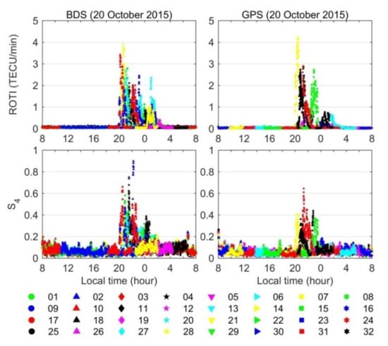
Figure 1.
Time series of the rate of TEC index (ROTI) and of different BDS and GPS satellites observed at Hong Kong Sha Tin (HKST) station on 20 October 2015 (day of year (DOY) 293). Different satellite pseudorandom noise (PRN) is represented by the different color or symbol as shown in the bottom side.
Statistical results of BDS scintillation in spring (March–May) and autumn (September–November) of 2015 are shown in this part. The selection of spring and autumn seasons of 2015 is based on two reasons. The first is that most BDS data from the Lands Department of the Government of Hong Kong Special Administrative Region (HKSAR) began in March of 2015. Another is the climatology characteristic of ionospheric scintillation occurrence in Hong Kong. Figure 2 shows four years (2013–16) statistics of scintillation in this region, which is represented by the GPS ROTI index derived from HKST station. It is clearly seen that most scintillation occurred in equinoctial seasons (spring and autumn). The intensity of scintillation is strongly associated with the solar activity. We can see that the scintillation in 2013–15 (high solar activity) is more significantly than that in 2016 (low solar activity). The above results are consistent to several previous studies [20,34]. In addition, it is also seen that the close relationship between the onset time of scintillation occurrence and the local sunset time. The detailed information can be seen in Luo et al. [29].
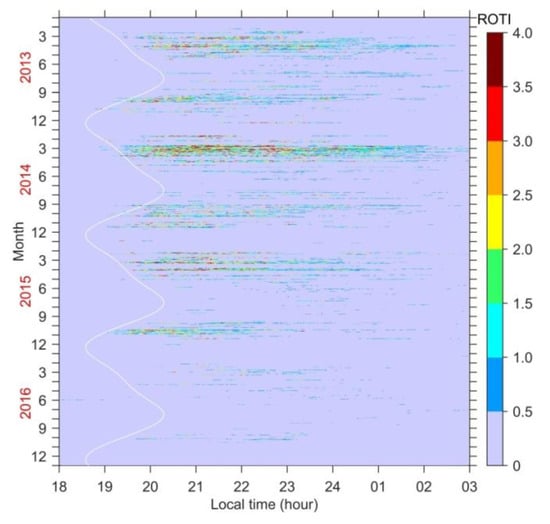
Figure 2.
Climatology characteristic of ionospheric scintillation in Hong Kong during 2013–16. The white line represents the local sunset time at 350 km altitudes.
Figure 3 presents the statistics of BDS and GPS scintillation observed at HKST station in spring and autumn of 2015. The data for 1–22 March is missing due to a data recording problem. Similar to previous study [35], the threshold of ROTI > 0.5 TECU/min is used to identify the scintillation event. The index is not used to identify the scintillation event because the value of derived from common geodetic GNSS receivers (30 s interval) is generally smaller than that released by the dedicated ISMRs. Specifically, the largest values close to 1 show an underestimation of around 10% compared with those from ISMRs [25]. The shown in this study is only used to display the relevant amplitude scintillation information due to the absence of BDS amplitude scintillation data from ISMRs. In the figure, the daily occurrence probability of scintillation is the ratio between the number of scintillation events and the total available epochs during 20:00–2:00 LT on each day.
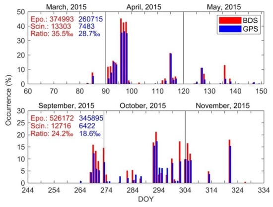
Figure 3.
Daily occurrence rate of BDS and GPS scintillation observed at HKST station in spring (March–May) and autumn (September–November) of 2015. The statistics of available epochs, scintillation events, and the corresponding ratio values are given in the top left corner of each panel.
From Figure 3, we can see that most ionospheric scintillations occur in April and October. Compared with GPS (blue bar), the occurrence probability of BDS scintillation (red bar) is more significant. The occurrence rate of BDS scintillation in spring and autumn are 35.5‰ and 24.2‰, respectively, which are larger than the values as 28.7‰ and 18.6‰ for GPS scintillation. It is well known that the satellite types of GPS system are MEO satellites. Relative to a static GNSS receiver, the GEO is almost static and the velocity of IGSO is around 1.8 km/s. Compared with GEO and IGSO, the velocity of MEO satellites can reach around 3.9 km/s. That is why GEO and IGSO scintillation show more significantly than MEO scintillation. Figure 4 further gives the daily occurrence rate of combined GEO and IGSO scintillation during the same two seasons in 2015. Due to only three BDS MEO satellites (C11, C12, and C14) during the considered period, we did not show the occurrence rate of BDS MEO separately. Figure 4 indicates that BDS GEO and IGSO scintillation are the majority of the BDS scintillation. Specifically, the occurrence rate of BDS GEO scintillation in spring and autumn account for 36.7‰ (6991/190,571) and 24.7‰ (6150/248,850), and the values of BDS IGSO scintillation account for 39.1‰ (5856/149,831) and 23.3‰ (6032/258,741), respectively. It is seen that the GEO scintillation occurrence rate is comparable to that of IGSO. Specifically, the occurrence rate of GEO scintillation is slighter smaller than that of IGSO scintillation in spring, while that in the autumn is opposite. From above analysis, we can conclude that the effects of ionospheric scintillation on BDS are generally more serious than the effects on GPS. Under scintillation conditions, several meters errors of positioning results have been shown in BDS PPP [21]. Therefore, next we try to seek the strategy to mitigate the scintillation effects on BDS PPP.
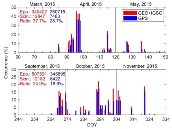
Figure 4.
Daily occurrence rate of combined geostationary Earth orbit (GEO) and inclined geosynchronous orbit (IGSO) scintillation observed at HKST station in spring (March–May) and autumn (September–November) of 2015.
2.3. Conventional Cycle-Slip Threshold
The TurboEdit algorithm is a famous cycle-slip detection method and is usually applied in GNSS data pre-processing [36]. It contains two basic detection observables, i.e., Melbourne-Wübbena (MW) wide-lane combination and geometry-free (GF) combination . Based on these two observables, the cycle-slip detection indicators can be calculated as:
where represents the data arc difference operator; is equal to ; is equal to .
Figure 5 shows a representative case of and fluctuation under ionospheric scintillation. The and are based on BDS data from HKST station on 20 October 2015. Each BDS satellite PRN can be referred to the color or symbol shown in the legend of Figure 1. We can find that during the non-scintillation period almost and keep a small and continuous variation within ±1 cycle and ±0.05 m. That is why the conventional threshold values as 1 cycle and 0.05 m for and observables are usually applied in GNSS PPP and RTK solutions [24,37]. During the scintillation period (20:00–2:00 LT), however, the time series of and fluctuate rapidly especially for those of . It is seen that most values of are larger than the threshold value as during 20:00–2:00 LT. From Equation (10), we can see that is associated with the ionospheric variation. During quiet ionospheric condition, the electron density of ionosphere shows smooth variation, so the value of is very small. However, inside the plasma irregularities, causing ionospheric scintillation occurrence, electron density with sharp gradients are existent. Those irregularities can result in rapid fluctuation of GNSS carrier-phase measurements. Therefore, we can see the obvious variation of the time series of during scintillation period in Figure 5. Although the fluctuation intensity of is weaker than that of , some values of during 20:00–2:00 LT are also larger than the typical threshold value as . The above analysis indicates that, under ionospheric scintillation, using the uniform thresholds such as 1 cycle and 0.05 m can induce a high false-alarm rate of cycle-slips especially using GF combination observable. Similar conclusion is also reported by several previous studies [24,38]. From Figure 5, we may also note that the fluctuation intensity of and generally depend on the scintillation level. Next we will take different scintillation levels into consideration to establish more appropriate cycle-slip thresholds.
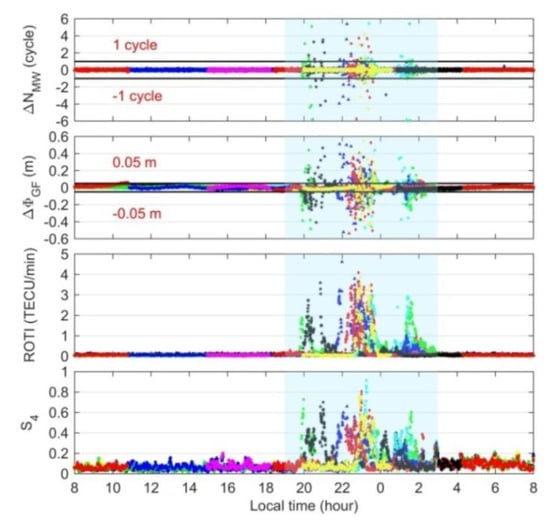
Figure 5.
Fluctuations of BDS , , ROTI, and for the HKST station on 20 October 2015 (DOY 293).
2.4. Cycle-Slip Threshold Model under Ionospheric Scintillation
To establish appropriate cycle-slip thresholds for BDS satellites data, one-year (from 23 March 2015 to 23 March 2016) distributions of and under different scintillation levels are given in Figure 6. For BDS GEO satellites, we can see that most values of and are smaller than 1.5 cycles and 0.4 m, but they show an increasing trend as the rise of scintillation levels when 0.5 < ROTI ≤ 3 TECU/min. In this ROTI range, we think that the thresholds of and can be modeled as polynomial expression. Under non-scintillation conditions as ROTI < 0.5 TECU/min or even ROTI < 0.1 TECU/min, we can find some anomalous and with large values ( > 3 cycles and > 0.6 m), which show the different characteristic compared to the values presented in Figure 5. Several researchers reported that cycle-slips are easily occurred in GEO carrier-phase measurements compared with IGSO and MEO even under normal ionospheric environment [38,39]. The second and third panels of Figure 6 also support such statement. After checking the GEO observations, it is found that the abrupt variation of phase observations is the single cycle-slip but is not associated with scintillation. Figure 7 presents a representative example of this kind of cycle-slip occurrence but without ionospheric scintillation. In the figure, cycle-slips are highlighted in the red ellipses with large values of and , which are detected in GEO C02 at 17:00:00 UT and C03 at 21:43:30 UT on 22 February 2016, respectively. This kind of cycle-slip can be caused by many factors like the interference [21]. It should be mentioned that, under normal ionospheric condition, the single cycle-slip occurred in GEO observations is infrequent. Statistics indicate that, when ROTI < 0.1 TECU/min, the number of > 0.05 m and > 1 cycle is only 1231 (0.03%) and 471 (0.01%) in total 4,024,233 data samples. Except for those anomalous values, most and keep stable variations under non-scintillation condition, so we think that the constant threshold is reasonable when ROTI < 0.5 TECU/min. For those ROTIs larger than 3 TECU/min, we also use constant thresholds in cycle-slip detection since the increasing trend of and are insignificant under such strong scintillation. From the above discussion, the cycle-slip thresholds of GEO and can be modeled by the piecewise function depended on ROTI index as shown in Equations (11) and (12).
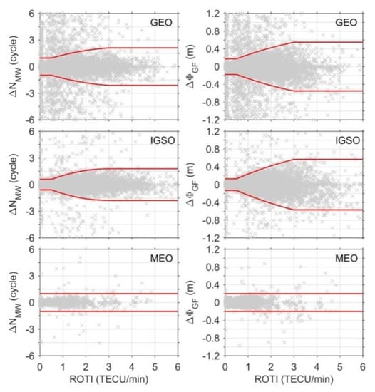
Figure 6.
Distribution of and against the scintillation index ROTI based on one-year BDS dataset from HKST. The red lines represent the cycle-slip thresholds relative to different ROTI values.
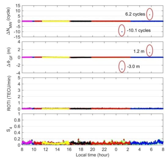
Figure 7.
Example of no scintillation occurrence but with cycle-slips using the BDS data collected at HKST station on 22 February 2016.
Note that a quadratic polynomial fitting is applied in the range of 0.5 < ROTI ≤ 3 TECU/min. Specifically, the original independent variable ROTI is selected based on each 0.05 TECU/min interval; and the original dependent variable or is selected based on 3 criterion (99.7%) for each ROTI interval. Figure 8 presents a typical example of the selection of ROTI, , and . In this case, as 0.975 < ROTI ≤ 1.025 TECU/min, the independent variable is calculated as , so the value as 1.0 TECU/min is selected. Meanwhile, the statistical characteristics of all and display the normal distribution and their standard deviation (STD) are 0.474 cycles and 0.093 m, respectively. Therefore, the values of 1.422 cycles (30.474) and 0.279 m (30.093) for and are selected as the dependent variables. Based on both independent and dependent variables, the polynomial coefficients can be calculated and the corresponding models can be established as shown in Equations (11) and (12).
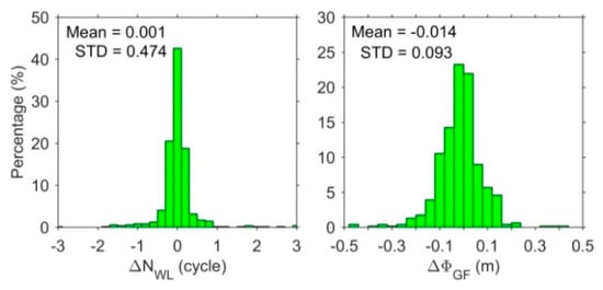
Figure 8.
Statistical characteristics of and for GEO satellites data when 0.975 < ROTI ≤ 1.025 TECU/min based on one-year BDS dataset from HKST.
The middle panels of Figure 6 indicate that the variations of IGSO and show similar characteristics to GEO satellites. Therefore, the thresholds of and for IGSO satellites data are also modeled using the same method as shown in Equations (11) and (12). The mathematical formulas of cycle-slip thresholds for IGSO satellites are given in Equations (13) and (14). For BDS MEO satellites, the constant values as 1 cycle and 0.2 m are selected since most and show stable variation within ±1 cycle and ±0.2 m relative to different ROTI values. It should be mentioned that the above models are based on one-year BDS dataset from the HKST station. The receiver type of HKST station is a Leica GR50 receiver. Cycle-slip thresholds for other GNSS receivers’ types also can be modeled in the same way.
3. Results
This section includes two parts. The first part presents the experimental data and scheme used to verify the availability of cycle-slip threshold models in BDS PPP solution. The second part shows the performance of our improved PPP solution in detail.
3.1. Data Resource and Experiment Scheme
To evaluate the availability of our proposed models, BDS dataset collected at 10 GNSS sites in Hong Kong from 1 September 2015 to 30 November 2015, are performed in the experiments. Figure 9 displays the geographical distribution of the 10 sites. All of them are installed with Leica GR50 receiver and they can track BDS satellite signals. In the data processing, the experimental demonstrations are processed in real-time mode with the FUSing IN Gnss (FUSING) software. This software is developed by the Wuhan University and is capable for the multi-frequency precise positioning, high-frequency satellite clock estimation and atmospheric modeling [40,41,42]. Table 1 gives the data processing methods for BDS PPP solution. In this study, the mitigated BDS PPP solution is based on the proposed threshold models as shown in Section 2.4, while the standard BDS PPP solution is based on the default threshold values as and .
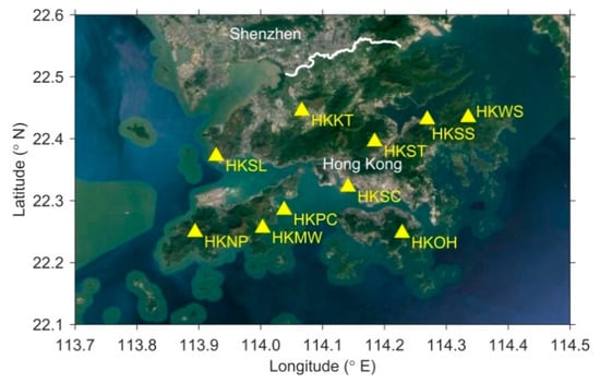
Figure 9.
Disturbation of 10 GNSS stations in Hong Kong.

Table 1.
Detailed information of BDS PPP solution.
3.2. Experiment and Analysis
Using the data collected at HKST station on 18, 19, and 20 October 2015 (DOYs 291, 292, and 293), we first present the positioning errors of standard and mitigated BDS PPP solutions under different scintillation conditions as shown in Figure 10. The RMS values are shown in the upper left corner of each positioning panels. Note that the RMS values shown in the top left are calculated by using the 4:00–24:00 UT (12:00–8:00 LT) results since the first several hours is in the state of convergence. For the continuous three days, the first day has no scintillation occurrence and the other two days have obvious scintillation but show different characteristics. From the ROTI panels, it can be seen that the peak of scintillation on DOY 292 occurred around 23:00 LT, while that on DOY 293 occurred around 20:40 LT. Note that the BDS satellite PRN can be referred to the legend of Figure 1. For the first day without scintillation, the time series of positioning results for two PPP solutions show quite stable variations after convergence. However, under scintillation conditions several meters error can be clearly seen in the standard PPP solution and the maximum variations occurred around the peak of scintillation time. Compared with standard PPP, we can observe that the mitigated PPP solution can effectively prevent the sudden variations of positioning errors induced by the ionospheric scintillation.
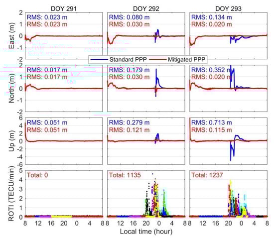
Figure 10.
BDS positioning results of standard and mitigated PPP solutions under different ionospheric environments on 18, 19, and 20 October 2015.
During the scintillation period, the rapid changes of positioning errors for the standard PPP should be associated with frequent cycle-slips occurrence due to the tight thresholds as and . Figure 11 shows the cycle-slips number detected in standard PPP (blue) and mitigated PPP (red) on DOYs 291, 292, and 293. The results of DOY 291 show that the cycle-slip number in mitigated PPP is 103, which is less than that in standard PPP with 350. We can find that the new threshold of GF combination is set to more flexible compared with the traditional threshold as shown in Section 2.4. Although the flexible threshold of GF would result in the misdetection of few real cycle-slips, it does not degrade the performance of mitigated PPP as shown in Figure 10 since most real cycle-slips can also be detected by the MW combination with tight threshold. The results on DOYs 292 and 293 clearly show that the number of cycle-slips in standard PPP is far more than that in mitigated PPP especially during the scintillation period. Statistical results indicate that on DOYs 292 and 293 the number of re-parameterized ambiguities for the standard PPP is 1399 and 1089, respectively, while that for the mitigated one is only 295 and 164. That means the proposed strategy can effectively avoid a larger number of unnecessary ambiguity resets. On DOYs 292 and 293, we may also note that few epochs of mitigated PPP results can reach several decimeters around the peak of scintillation time. That is because the improved strategy mainly focuses on reducing the number of misjudged cycle-slips instead of repairing the real cycle-slips caused by the ionospheric scintillation. In these cases, an alternative strategy is to enhance the performance of GNSS receivers. In addition, avoiding the use of GNSS measurements with successive losses of lock in the presence of strong scintillation also can mitigate the remaining degradations [27]. However, the premise is that the number of available satellites should be sufficient. Even though few degraded results appeared in the mitigated PPP solution, RMS statistics show much smaller than those of standard PPP solution.
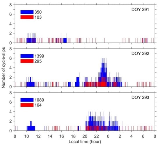
Figure 11.
Number of cycle-slips for HKST station on 18, 19, and 20 October 2015. The blue bar shows the result of standard approach, and the red one shows the corresponding result of mitigated approach. The total number of cycle-slips is given in the upper left corner.
Using the BDS dataset collected at HKST site, the detailed daily RMS statistics (from 1 September to 30 November in 2015) of positioning errors for the standard PPP and mitigated PPP solutions are shown in Figure 12. The corresponding mean values of RMS are shown in the upper left corner. The daily total scintillation events (ROTI > 0.5 TECU/min) are also given in the fourth panel of Figure 12. Because of the problem of BDS precise products on DOYs 283 and 284, we did not show the result for the two days. As shown in the fourth panel of Figure 12, total 23 days BDS data encountered obvious ionospheric scintillation effects. According to the RMS statistics, the positioning results of standard PPP on scintillation days are generally larger than those on non-scintillation days. However, we also note that not all ionospheric scintillations result in serious degradation of PPP performance. For example, the results on DOY 274 with 220 scintillation events are comparable to those on DOY 275 without scintillation effects. ROTI and indices of DOY 274 indicates that only three BDS satellites (C02, C03, and C10) encountered scintillation effects; meanwhile, all of them are smaller than 2 TECU/min and 0.5, respectively. That means the scintillation on DOY 274 is insignificant. Previous study has demonstrated that the weak scintillation (0.2 < ≤ 0.6) only results in the increasing measurement noise instead of loss of signal lock [20]. Thus, in Figure 12, it is found that under non-scintillation or insignificant scintillation conditions, the results of standard PPP and mitigated PPP are comparable. The values of RMS 3D for the two PPP solutions are smaller than 0.2 m. On the strong scintillation days (DOYs 269, 292, 293, 299, 302, 304, 305 and 321), the mitigated PPP solution can significantly improve positioning accuracy compared with the standard PPP. The values of RMS 3D are better than 0.25 m, further indicating the availability of our proposed method.
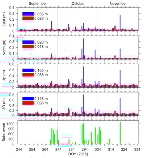
Figure 12.
RMS statistics of standard BDS PPP (blue) and mitigated PPP (red) in the east, north, up, and 3D directions under different ionospheric scintillation (green) from 1 September to 30 November 2015. The corresponding mean RMS values are shown in the upper left corner.
The above analyses are only based on the data from HKST station. To further verify the serviceability of our mitigated solution, three months (from 1 September 2015 to 30 November 2015) dataset collected at 10 GNSS stations (see Figure 9) are performed in the following experiments. Figure 13 presents the detailed comparison of positioning results for the standard PPP (upper panels) and mitigated PPP (bottom panels) solutions on 20 October 2015 (DOY 293). From Figure 13, it is clearly seen that the standard PPP of all stations were affected by the ionospheric scintillation. The corresponding mean RMS values are 0.404 m and 0.920 m in the horizontal and vertical directions, respectively. Note that the total number of scintillation events on DOY 293 is 1237, which is the strong scintillation day during the three months. As mentioned before, the spatial scale of equatorial plasma irregularities can reach several hundred kilometers [7,8,9,10], while the horizontal scale of Hong Kong is only around 60 km. That is why all stations in Hong Kong region show positioning degradation under strong scintillation conditions on DOY 293. From the bottom panel of Figure 13, we can find that our mitigated solution can effectively reduce the scintillation effects for all stations. The corresponding mean RMS values are only 0.049 m (horizontal) and 0.133 m (vertical).
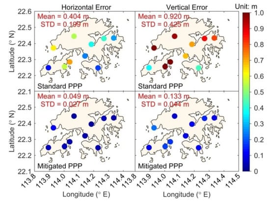
Figure 13.
Positioning results of standard BDS PPP (upper panels) and mitigated BDS PPP (bottom panels) in the horizontal and vertical components on 20 October 2015 (DOY 293).
A comprehensive comparison between two PPP solutions is shown in Figure 14. The results are based on BDS dataset collected by 10 stations from 1 September 2015 to 30 November 2015. The color bar gives the positioning errors in 3D direction. In addition, the RMS statistics are shown in the upper left corner in Figure 14. For the standard PPP, we can clearly observe that positioning errors of several meters appeared in different directions and the maximum can reach around 6 m. Those results are consistent with Figure 10. The corresponding RMS values are 0.104 m and 0.190 m in the horizontal and vertical components, respectively. For the mitigated PPP, the positioning errors show more concentrated distribution. Statistical results indicate that the mitigated PPP maintains an accuracy of 0.073 m (horizontal) and 0.099 m (vertical). Compared with the standard one, the positioning accuracy of our proposed strategy is improved by approximately 24.1%, 38.2%, and 47.9% in the east, north, and up directions, respectively. Although significant improvement for the mitigated solution is shown in the experiment, we may also note that the magnitude of RMS values for the two solutions are comparable. That is because the degraded positioning results of standard PPP only occurred in the local nighttime as 20:00–2:00 LT, which means the affected data accounts for a minority in all day data.
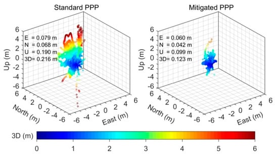
Figure 14.
Distribution of positioning errors in the east, north, and up directions for the standard PPP and mitigated PPP using BDS satellites data collected by 10 GNSS stations from 1 September 2015 to 30 November 2015. The corresponding RMS values are shown in the upper left corner.
4. Discussion
The cycle-slip threshold model shown in this study can decrease the false-alarm rate of BDS cycle-slips caused by the ionospheric scintillation, thus avoiding frequent unnecessary ambiguity resets in BDS PPP solution (see Figure 11). Encouraging results have been presented in Figure 10, Figure 12, Figure 13 and Figure 14. From Equations (11)–(14), it can be clearly seen that the thresholds of and in our model are more flexible than the conventional thresholds as and . That means we will miss some real cycle-slips under scintillation conditions. Compared with some omission of real cycle-slips, a large number of “wrong cycle-slips” determined by the traditionally tight thresholds will degrade the GNSS PPP performance more seriously. That is why some studies chose to enlarge the cycle-slip thresholds [24] and even turn off the GF combination method [44] in GNSS PPP solution. Note that although significant improvement has been shown in BDS PPP, the mitigated strategy shown in this study cannot resolve the real cycle-slips. One feasible way is to detect and correct them before PPP processing [36,45]. However, repairing the cycle-slip is a difficult task using the 30 s sampling interval data especially in strong ionospheric activity condition. It also should be mentioned that the performance of our proposed strategy can also be affected by the number of data gaps caused by losses of signal lock since we did not consider the method to connect the data gaps yet. Several studies have been reported that, under extreme space weather event like the geomagnetic storm, several satellites may encounter losses of signal lock [46,47,48]. In this case, Banville and Langley [49] proposed a three-step method to estimate the size of signal interruption (cycle-slip) based on LAMBDA method in real-time kinematic PPP. The success rate of cycle-slip correction for 1 s interval data can reach around 100%, but it shows dramatic decrease as data gaps occur because of the temporal decorrelation of different errors such as atmospheric delay and phase wind-up effects. Zhang and Li [50] further presented that the data gaps of up to 300 s can also be connected successfully after refining and isolating the different errors from integer cycle-slips. Note that the former two studies are based on the GPS data with simulated cycle-slips and data gaps. Under real losses of lock effects, feasible strategies including avoiding the use of GNSS measurements with successive losses of lock [27] and combining multi-GNSS data to enhance the satellite geometry [51].
In this study, the BDS dual-frequency datasets used for modeling the cycle-slip are derived from Leica GR50 receivers. To keep consistency, Leica GR50 receiver data is also performed in our BDS PPP experiments as we mentioned in Section 3.1. It is well known that due to the different hardware and signal tracking algorithms, GNSS receivers under ionospheric scintillation can show different performance. For example, McCaffrey et al. [52] reported that the Septentrio PolaRxS Pro receiver presents a better carrier-phase tracking ability than the Trimble NetR9 under ionospheric scintillation. It also should be mentioned that all experimental datasets are come from Hong Kong in 2015. That is because: 1. Hong Kong is located at low-latitudes with frequent ionospheric scintillation occurrence; 2. In 2015, only the GNSS receivers in Asia-Pacific can track almost all BDS satellites signals; 3. At low-latitudes, ionospheric scintillation occur frequently in solar maximum years like the year of 2015. Taking the above factors into account, we therefore select the Hong Kong data to conduct experiments. Note that our proposed strategy also can be applied in other low-latitude areas of Asia-Pacific. Figure 15 further presents the results of mitigated PPP using BDS data from three stations located at different geomagnetic latitudes. They are LALX (18.2°N, 105.0°E; MLAT: 11.3°N) in Loas, YONG (16.8°N, 112.3°E; MLAT: 9.9°N) in Yongxing Island in the South China Sea, and SIN1 (1.3°N, 103.7°E; MLAT: 7.2°S) in Singapore, which are situated in EIA regions. It also should be mentioned that these stations are installed with the Trimble NetR9 receiver. Similar to previous results in Figure 10, Figure 12, Figure 13 and Figure 14, Figure 15 also demonstrates the availability of our proposed approach.
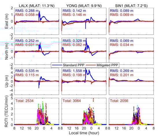
Figure 15.
BDS Positioning results of standard and mitigated PPP solutions for different area stations as LALX, YONG, and SIN1 on 13 March 2015 (DOY 72).
Compared with BDS, others GNSS systems such as GPS, GLONASS, and Galileo are made up of the single satellite type, i.e., MEO satellite. From this point of view, the proposed strategy in this study can be easily applied in those systems since we only need to consider the single MEO satellite data instead of multi-types satellite data like BDS GEO and IGSO into modeling. We may note that MEO satellites also include several types. For example, with the modernization of GPS, its constellation is made up of the Block IIA, IIR, IIR-M, and IIF satellites (https://www.gps.gov/). That means the further robust method can take several types of MEO satellite data into consideration. The other point is the difference magnitude of ROTI derived from different GNSS measurements when we use the index ROTI to represent scintillation intensity as shown in our cycle-slip threshold model. Liu et al. [53] reported that for the same GNSS receiver, the inconsistency of ROTI for GPS and BDS can reach around 0.5 TECU/min. For this case, our proposed strategy is still valid as long as establishing the relationship between the cycle-slip threshold and the ROTI magnitude.
More robust cycle-slip threshold model using the GNSS data from several categories receivers and different regions needs further investigation. Nevertheless, this study provides several new points in the study of BDS/GNSS scintillation at low-latitudes. First of all, scintillation properties of BDS and GPS satellites tracked by the common geodetic receivers are detailed presented and explained. We demonstrate that BDS GEO and IGSO satellite signals are more easily affected by the scintillation compared with GPS MEO satellite signals. Second, for the first time, we propose an effective strategy to mitigate scintillation effects on BDS PPP technique through establishing cycle-slip threshold model. Different from previous cycle-slip thresholds, new modeled thresholds are established based on the scintillation index. Most importantly, the mitigation approach shown in this study is based on common GNSS receiver data. As far as we known, the famous tracking jitter model [26] and the recently proposed scintillation effects model [27] must rely on dedicated ISMRs with high-rate data. From this point of view, our proposed strategy should be more practical and can further extend GNSS scintillation study, especially for China’s BDS.
5. Conclusions
The effects of ionospheric scintillation on BDS system are generally more serious than the GPS because of the special design of BDS constellation. Using six months of data collected at HKST station during spring (March–May) and autumn (September–November) in the year 2015, we show that the BDS scintillation events account for 35.5‰ and 24.2‰ in spring and autumn equinoxes respectively, while the percentages of GPS scintillation events are only 28.7‰ and 18.6‰. As BDS is currently providing global services, it is increasingly important to seek strategies to mitigate the ionospheric scintillation effects on BDS.
This study presents an improved cycle-slip threshold model to decrease the false-alarm rate of cycle-slips detection under ionospheric scintillation conditions, thus avoiding the frequent unnecessary ambiguity resets in PPP solution. Using one-year BDS dataset collected at HKST station from 23 March 2015 to 23 March 2016, the cycle-slip threshold model is established in this study. Different from the traditional empirical threshold, the threshold model takes different types of BDS satellites and multiple scintillation levels into consideration, thereby making the processing of cycle-slip detection more robust in BDS PPP. The availability of our proposed strategy is conducted by using three months (from 1 September 2015 to 30 November 2015) dataset derived from 10 GNSS stations in Hong Kong. Positioning results clearly indicate that the mitigated BDS PPP can decrease the sudden variations of positioning errors induced by the ionospheric scintillation. Long-term statistics show that the mitigated PPP solution maintains an accuracy of about 0.08 m and 0.10 m in the horizontal and vertical components, respectively. Compared with the standard BDS PPP, the positioning accuracy of the mitigated one is improved by approximately 24.1%, 38.2%, and 47.9% in the east, north, and up directions, respectively.
Author Contributions
Methodology, Y.L., S.G. and X.L.; software, S.G. and X.L.; validation, X.L. and S.G.; data curation, X.L.; writing—original draft, X.L.; writing—review and editing, X.L., Y.L., S.G. and W.S.; supervision, Y.L., S.G. and W.S.
Funding
This research was funded by the National Key Research and Development Program of China (Nos. 2018YFC1503502, 2017YFB0503401 and 2016YFB0501802). This study was supported by the State Grid Corporation Science and Technology Project (Grant No. 5211XT180047).
Acknowledgments
We thank the HKSAR, CMONOC, and IGS for providing the BDS data and the GFZ for providing precise orbit and clock products. We appreciate the very helpful guidance and suggestion from Biyan Chen and Muhammad Bilal. The authors are also thankful the four reviewers for giving constructive comments on this paper.
Conflicts of Interest
The authors declare no conflict of interest.
References
- CSNO. BeiDou Navigation Satellite System Signal in Space Interface Control Document, Open Service Signal B1I, Version 3.0; China Satellite Navigation Office: Beijing, China, 2019.
- Shi, C.; Zhao, Q.; Hu, Z.; Liu, J. Precise relative positioning using real tracking data from COMPASS GEO and IGSO satellites. GPS Solut. 2013, 17, 103–119. [Google Scholar] [CrossRef]
- Zhang, R.; Tu, R.; Liu, J.; Hong, J.; Fan, L.; Zhang, P.; Lu, X. Impact of BDS-3 experimental satellites to BDS-2: Service area, precise products, precise positioning. Adv. Space Res. 2018, 62, 829–844. [Google Scholar] [CrossRef]
- Tang, W.; Jin, L.; Xu, K. Performance analysis of ionosphere monitoring with BeiDou CORS observational data. J. Navig. 2014, 67, 511–522. [Google Scholar] [CrossRef]
- Appleton, E.V. Two anomalies in the ionosphere. Nature 1946, 157, 691. [Google Scholar] [CrossRef]
- Luo, W.; Zhu, Z.; Xiong, C.; Chang, S. The response of equatorial ionization anomaly in 120°E to the geomagnetic storm of 18 August 2003 at different altitudes from multiple satellite observations. Space Weather 2017, 15, 1588–1601. [Google Scholar] [CrossRef]
- Woodman, R.F.; La Hoz, C. Radar observations of F region equatorial irregularities. J. Geophys. Res. 1976, 81, 5447–5466. [Google Scholar] [CrossRef]
- Basu, S.; Basu, S.; Aarons, J.; Mcclure, J.P.; Cousins, M.D. On the coexistence of kilometer- and meter-scale irregularities in the nighttime equatorial F region. J. Geophys. Res. 1978, 83, 4219–4226. [Google Scholar] [CrossRef]
- Kil, H.; Heelis, R.A. Equatorial density irregularity structures at intermediate scales and their temporal evolution. J. Geophys. Res. 1998, 103, 3969–3981. [Google Scholar] [CrossRef]
- Smith, J.; Heelis, R.A. Equatorial plasma bubbles: Variations of occurrence and spatial scale in local time, longitude, season, and solar activity. J. Geophys. Res. Space Phys. 2017, 122, 5743–5755. [Google Scholar] [CrossRef]
- Crane, R.K. Ionospheric scintillation. Proc. IEEE 1997, 65, 180–199. [Google Scholar] [CrossRef]
- Zumberge, J.F.; Heftin, M.B.; Jefferson, D.; Watkins, M.M.; Webb, F.H. Precise point positioning for the efficient and robust analysis of GPS data from large networks. J. Geophys. Res. 1997, 102, 5005–5017. [Google Scholar] [CrossRef]
- Skone, S.; Knudsen, K.; de Jong, M. Limitations in GPS receiver tracking performance under ionospheric scintillation conditions. Phys. Chem. Earth Part A Solid Earth Geod. 2001, 26, 613–621. [Google Scholar] [CrossRef]
- Aquino, M.; Moore, T.; Dodson, A.; Waugh, S.; Souter, J.; Rodrigues, F.S. Implications of ionospheric scintillation for GNSS users in northern Europe. J. Navig. 2005, 58, 241–256. [Google Scholar] [CrossRef]
- Xu, R.; Liu, Z.; Li, M.; Morton, Y.; Chen, W. An analysis of low-latitude ionospheric scintillation and its effects on precise point positioning. J. Glob. Position. Syst. 2012, 11, 22–32. [Google Scholar] [CrossRef]
- Moreno, B.; Radicella, S.; de Lacy, M.C.; Herraiz, M.; Rodriguez-Caderot, G. On the effects of the ionospheric disturbances on precise point positioning at equatorial latitudes. GPS Solut. 2011, 15, 381–390. [Google Scholar] [CrossRef]
- Dubey, S.; Wahi, R.; Gwal, A.K. Ionospheric effects on GPS positioning. Adv. Space Res. 2006, 38, 2478–2484. [Google Scholar] [CrossRef]
- Aquino, M.; Monico, J.F.G.; Dodson, A.H.; Marques, H.; de Franceschi, G.; Alfonsi, L.; Romano, V.; Andreotti, M. Improving the GNSS positioning stochastic model in the presence of ionospheric scintillation. J. Geod. 2009, 83, 953–966. [Google Scholar] [CrossRef]
- He, Z.; Zhao, H.; Feng, W. The ionospheric scintillation effects on the BeiDou signal receiver. Sensors 2016, 16, 1883. [Google Scholar] [CrossRef]
- Luo, X.; Liu, Z.; Lou, Y.; Gu, S.; Chen, B. A study of multi-GNSS ionospheric scintillation and cycle-slip over Hong Kong region for moderate solar flux conditions. Adv. Space Res. 2017, 60, 1039–1053. [Google Scholar] [CrossRef]
- Luo, X.; Lou, Y.; Xiao, Q.; Gu, S.; Chen, B.; Liu, Z. Investigation of ionospheric scintillation effects on BDS precise point positioning at low-latitude regions. GPS Solut. 2018, 22, 63. [Google Scholar] [CrossRef]
- Park, J.; Veettil, S.V.; Aquino, M.; Yang, L.; Cesaroni, C. Mitigation of ionospheric effects on GNSS positioning at low latitudes. J. Inst. Navig. 2017, 64, 67–74. [Google Scholar] [CrossRef]
- da Silva, H.A.; de Oliveira Camargo, P.; Galera Monico, J.F.; Aquino, M.; Marques, H.A.; de Franceschi, G.; Dodson, A. Stochastic modelling considering ionospheric scintillation effects on GNSS relative and point positioning. Adv. Space Res. 2010, 45, 1113–1121. [Google Scholar] [CrossRef]
- Zhang, X.; Guo, F.; Zhou, P. Improved precise point positioning in the presence of ionospheric scintillation. GPS Solut. 2014, 18, 51–60. [Google Scholar] [CrossRef]
- Juan, J.M.; Sanz, J.; González-Casado, G.; Rovira-Garcia, A.; Camps, A.; Riba, J.; Barbosa, J.; Blanch, E.; Altadill, D.; Orus, R. Feasibility of precise navigation in high and low latitude regions under scintillation conditions. J. Space Weather Space Clim. 2018, 8, A05. [Google Scholar] [CrossRef]
- Conker, R.S.; El-Arini, M.B.; Hegarty, C.J.; Hsiao, T. Modeling the effects of ionospheric scintillation on GPS/Satellite-based augmentation system availability. Radio Sci. 2003, 38, 1–23. [Google Scholar] [CrossRef]
- Vani, B.C.; Forte, B.; Monico, J.F.G.; Skone, S.; Shimabukuro, M.H.; Moraes, A.O.; Portella, I.P.; Marques, H.A. A novel approach to improve GNSS Precise Point Positioning during strong ionospheric scintillation: Theory and demonstration. IEEE Trans. Veh. Technol. 2019, 68, 4391–4403. [Google Scholar] [CrossRef]
- Gu, S.; Lou, Y.; Shi, C.; Liu, J. BeiDou phase bias estimation and its application in precise point positioning with triple-frequency observable. J. Geod. 2015, 89, 979–992. [Google Scholar] [CrossRef]
- Luo, X.; Xiong, C.; Gu, S.; Lou, Y.; Stolle, C.; Wan, X.; Liu, K.; Song, W. Geomagnetically conjugate observations of equatorial plasma irregularities from swarm constellation and ground-based GPS stations. J. Geophys. Res. Space Phys. 2019, 124, 3650–3665. [Google Scholar] [CrossRef]
- Pi, X.; Mannucci, A.J.; Lindqwister, U.J.; Ho, C.M. Monitoring of global ionospheric irregularities using the worldwide GPS network. Geophys. Res. Lett. 1997, 24, 2283–2286. [Google Scholar] [CrossRef]
- Lou, Y.; Luo, X.; Gu, S.; Xiong, C.; Song, Q.; Chen, B.; Xiao, Q.; Chen, D.; Zhang, Z.; Zheng, G. Two typical ionospheric irregularities associated with the tropical cyclones Tembin (2012) and Hagibis (2014). J. Geophys. Res. Space Phys. 2019, 124, 1–16. [Google Scholar] [CrossRef]
- Van Dierendonck, A.J.; Klobuchar, J.; Hua, Q. Ionospheric scintillation monitoring using commercial single frequency C/A code receivers. In Proceedings of the 6th International Technical Meeting of the Satellite Division of The Institute of Navigation (ION GPS 1993), Salt Lake City, UT, USA, 22–24 September 1993; pp. 1333–1342. [Google Scholar]
- Kintner, P.M.; Ledvina, B.M.; de Paula, E.R. GPS and ionospheric scintillations. Space Weather 2007, 5, S09003. [Google Scholar] [CrossRef]
- Liu, K.; Li, G.; Ning, B.; Hu, L.; Li, H. Statistical characteristics of low-latitude ionospheric scintillation over China. Adv. Space Res. 2015, 55, 1356–1365. [Google Scholar] [CrossRef]
- Ma, G.; Maruyama, T. A super bubble detected by dense GPS network at East Asian longitudes. Geophys. Res. Lett. 2006, 33, L21103. [Google Scholar] [CrossRef]
- Blewitt, G. An automatic editing algorithm for GPS data. Geophys. Res. Lett. 1990, 17, 199–202. [Google Scholar] [CrossRef]
- Chen, D.; Ye, S.; Zhou, W.; Liu, Y.; Jiang, P.; Tang, W.; Yuan, B.; Zhao, L. A double-differenced cycle slip detection and repair method for GNSS CORS network. GPS Solut. 2016, 20, 439–450. [Google Scholar] [CrossRef]
- Ju, B.; Gu, D.; Chang, X.; Herring, T.A.; Duan, X. Enhanced cycle slip detection method for dual-frequency BeiDou GEO carrier phase observations. GPS Solut. 2017, 21, 1227–1238. [Google Scholar] [CrossRef]
- Montenbruck, O.; Steigenberger, P.; Khachikyan, R.; Weber, G.; Langley, R.B.; Mervart, L.; Hugentobler, U. IGS-MGEX: Preparing the ground for multi-constellation GNSS science. Inside GNSS 2014, 9, 42–49. [Google Scholar]
- Shi, C.; Guo, S.; Gu, S.; Yang, X.; Gong, X.; Deng, Z.; Ge, M.; Schuh, H. Multi-GNSS satellite clock estimation constrained with oscillator noise model in the existence of data discontinuity. J. Geod. 2019, 93, 515–528. [Google Scholar] [CrossRef]
- Yang, X.; Gu, S.; Gong, X.; Song, W.; Lou, Y.; Liu, J. Regional BDS satellite clock estimation with triple-frequency ambiguity resolution based on undifferenced observation. GPS Solut. 2019, 23, 1–11. [Google Scholar] [CrossRef]
- Zhao, Q.; Wang, Y.; Gu, S.; Zheng, F.; Shi, C.; Ge, M.; Schuh, H. Refining ionospheric delay modeling for undifferenced and uncombined GNSS data processing. J. Geod. 2019, 93, 545–560. [Google Scholar] [CrossRef]
- Hopfield, H.S. Tropospheric effect on electromagnetically measured range: Prediction from surface weather data. Radio Sci. 1971, 6, 357–367. [Google Scholar] [CrossRef]
- Rodríguez-Bilbao, I.; Radicella, S.M.; Rodríguez-Caderot, G.; Herraiz, M. Precise point positioning performance in the presence of the 28 October 2003 sudden increase in total electron content. Space Weather 2015, 13, 698–708. [Google Scholar] [CrossRef]
- Liu, Z. A new automated cycle slip detection and repair method for a single dual-frequency GPS receiver. J. Geod. 2011, 85, 171–183. [Google Scholar] [CrossRef]
- Astafyeva, E.; Yasyukevich, Y.; Maksikov, A.; Zhivetiev, I. Geomagnetic storms, super-storms, and their impacts on GPS-based navigation systems. Space Weather 2014, 12, 508–525. [Google Scholar] [CrossRef]
- Xiong, C.; Stolle, C.; Lühr, H. The Swarm satellite loss of GPS signal and its relation to ionospheric plasma irregularities. Space Weather 2016, 14, 563–577. [Google Scholar] [CrossRef]
- Luo, X.; Gu, S.; Lou, Y.; Xiong, C.; Chen, B.; Jin, X. Assessing the performance of GPS precise point positioning under different geomagnetic storm conditions during solar cycle 24. Sensors 2018, 18, 1784. [Google Scholar] [CrossRef]
- Banville, S.; Langley, R.B. Improving real-time kinematic PPP with instantaneous cycle-slip correction. In Proceedings of the ION GNSS 2009, Savannah, GA, USA, 22–25 September 2009; pp. 2470–2478. [Google Scholar]
- Zhang, X.; Li, X. Instantaneous re-initialization in real-time kinematic PPP with cycle slip fixing. GPS Solut. 2012, 16, 315–327. [Google Scholar]
- Marques, H.A.; Marques, H.A.S.; Aquino, M.; Veettil, S.V.; Monico, J.F.G. Accuracy assessment of precise point positioning with multi-constellation GNSS data under ionospheric scintillation effects. J. Space Weather Space Clim. 2018, 8, A15. [Google Scholar] [CrossRef]
- McCaffrey, A.M.; Jayachandran, P.T.; Langley, R.B.; Sleewaegen, J.M. On the accuracy of the GPS L2 observable for ionospheric monitoring. GPS Solut. 2018, 22, 23. [Google Scholar] [CrossRef]
- Liu, Z.; Yang, Z.; Xu, D.; Morton, Y.J. On inconsistent ROTI derived from multiconstellation GNSS measurements of globally distributed GNSS receivers for ionospheric irregularities characterization. Radio Sci. 2019, 54, 215–232. [Google Scholar] [CrossRef]


© 2019 by the authors. Licensee MDPI, Basel, Switzerland. This article is an open access article distributed under the terms and conditions of the Creative Commons Attribution (CC BY) license (http://creativecommons.org/licenses/by/4.0/).