Mapping and Monitoring Fractional Woody Vegetation Cover in the Arid Savannas of Namibia Using LiDAR Training Data, Machine Learning, and ALOS PALSAR Data

Abstract

Namibia is a very arid country, which has experienced significant bush encroachment and associated decreased livestock productivity. Therefore, it is essential to monitor bush encroachment and widespread debushing activities, including selective bush thinning and complete bush clearing. The aim of study was to develop a system to map and monitor fractional woody cover (FWC) at national scales (50 m and 75 m resolution) using Synthetic Aperture Radar (SAR) satellite data (Advanced Land Observing Satellite (ALOS) Phased Arrayed L-band Synthetic Aperture Radar (PALSAR) global mosaics, 2009, 2010, 2015, 2016) and ancillary variables (mean annual precipitation—MAP, elevation), with machine learning models that were trained with diverse airborne Light Detection and Ranging (LiDAR) data sets (244,032 ha, 2008–2014). When only the SAR variables were used, an average R² of 0.65 (RSME = 0.16) was attained. Adding either elevation or MAP, or both ancillary variables, increased the mean R² to 0.75 (RSME = 0.13), and 0.79 (RSME = 0.12). The inclusion of MAP addressed the overestimation of FWC in very arid areas, but resulted in anomalies in the form of sharp gradients in FWC along a MAP contour which were most likely caused by to the geographic distribution of the LiDAR training data. Additional targeted LiDAR acquisitions could address this issue. This was the first attempt to produce SAR-derived FWC maps for Namibia and the maps contain substantially more detailed spatial information on woody vegetation structure than existing national maps. During the seven-year study period the Shrubland–Woodland Mosaic was the only vegetation structural class that exhibited a regional net gain in FWC of more than 0.2 across 9% (11,906 km²) of its area that may potentially be attributed to bush encroachment. FWC change maps provided regional insights and detailed local patterns related to debushing and regrowth that can inform national rangeland policies and debushing programs.

1. Introduction

Savannas have been described as “communities or landscapes with a continuous grass layer and a discontinuous tree layer” [1]. Savannas are complex and structurally diverse ecosystems, both in terms of the varying proportions, spatial distributions, and architectures of tree, shrub, and grass cover at varying stages of growth [2]. The woody cover in these tree–grass communities are determined by water availability, nutrient availability, fire and herbivory, as well as interactions between these drivers [3]. Savannas occupy approximately 20% of the global land surface and occur largely in the tropics and sub-tropics [4]. Although the carbon density of savannas and woodlands is lower than that of dense forests, in Africa 52% of the total above-ground carbon is stored in savannas and woodlands, and 48% in dense forests (including mangroves and flooded forests) [5]. Savannas furthermore contain a large proportion of the world’s human population and the majority of its livestock and wildlife [1,6].

Globally, woody cover in savannas and grasslands has increased [7,8,9,10,11]. Whether the widespread increase in woody cover are driven by local or global drivers is a highly contentious issue [8,11,12]. Local drivers of encroachment include fire suppression, livestock grazing pressure, historical loss of browsing herbivores, wildlife and livestock pandemics (such as rinderpest), as well as interactions between fire and rainfall episodes [13,14]. Evidence now suggests that global increases in atmospheric carbon dioxide may play a greater role in this than previously thought [7,8,9,10].

Given the vast extent of savannas, changes in the tree–grass balance at regional scales could have large feedbacks to the earth–atmosphere system [15,16,17]. At local to landscape scale the tree–grass dynamics have a large impact on rangeland use, wildlife-based tourism, biodiversity, and ecosystem function, such as hydrology and nutrient cycling [3,18]. In southern Africa bush encroachment causes a large amount of rainfall to be intercepted and transpired back into the atmosphere. Less water is then available to grass plants that could produce fodder for grazing animals. Together with increased water use, this results in a loss in carrying capacity and productive use of rangelands for both cattle and game [9,19,20]. The conventional understanding of the local drivers of bush encroachment in Namibia are the prolonged denudation of soils caused by droughts and grazing, followed by above-average rainfall years with frequent rainfall events, favoring mass tree recruitment [19]. However, it has been argued that there is very limited evidence from field data to support this conventional understanding of the drivers of bush encroachment [20]. A more complex state-and-transition model has been proposed to explain the thickening of bush in the Highland savanna of Namibia, according to which seedlings are established episodically following three consecutive years of above-average rainfall, facilitated by low grass biomass, but suppressed by fire [21].

Nearly 50% of the commercial rangeland areas of Namibia are believed to be affected by bush encroachment [22,23], mainly concentrated in areas with about 300–500 mm annual rainfall (Figure 1A,B) [19]. Bush encroachment affects approximately 26 million ha (260,000 to 300,000 km²) of woodland savannas in Namibia and results in a loss of animal production of as much as 100% in the worst affected areas, which amounts to N$700 million in lost meat production annually [19,24]. This threatens the livelihood of both commercial and communal game and livestock ranchers which accounts for 70% of Namibia’s agricultural sector [22]. Consequently, debushing activities (including selective bush thinning and complete bush clearing) are being promoted by national policy, such as the National Development Plan NDP 5 (National Planning Commission, 2017) and the Namibia Rangeland Management Policy and Strategy [25], as well as large international donor-funded projects (such as Deutsche Gesellschaft für Internationale Zusammenarbeit (GIZ) project “Utilizing Bush Biomass in Namibia” https://www.giz.de/en/worldwide/28648.html). The bush encroachment also presents an opportunity to use this woody vegetation resource to create jobs and economic growth. The largest use of the wood biomass is for fuelwood as 440,000 t of wood are used annually for own household consumption and another 45,000 t/yr is sold formally, while 60,000–160,000 t of charcoal are exported annually [26]. Significant potential also lies in the energy use of bush biomass, both in industrial applications (e.g., powering of steam turbines) and biomass power plants (e.g., 5–20 MW plants) [27]. Despite all the scientific interest, the economic impacts, and national-level initiatives concerned with bush encroachment, there is surprisingly little spatial information on woody vegetation distribution and structure [26]. An estimated 120,000 ha of land is debushed annually by chemical and mechanical means [26], but there is no systematic monitoring of debushing activities. Estimates of the spatial distribution of bush encroachment are based on a map created from field surveys that date back to 1996–1999 [24] and remains the only country-wide spatial data set on which policy and debushing initiatives are based. The current study therefore endeavored to develop a reliable system to map and monitor woody vegetation cover with the most advanced, yet affordable remote sensing technology.

Methods for mapping and monitoring woody vegetation and specifically bush encroachment have relied on field work [10,13,24], historical photographs [14], historical aerial photographs [8,10,28], and satellite data. Optical satellite data have been used in diverse approaches to map woody vegetation structure, but most studies are focused on high biomass, tropical forest monitoring [29,30] while limited remote sensing studies focused on dryland woody vegetation [31,32]. Bastin et al. [31] recently revealed that the extent of global dryland forests (tree canopy cover > 10%), in particular in southern Africa, was 40–47% higher than previously estimated by remotely sensed global, forest maps [29,30]. Within sub-Saharan Africa there have been several studies using optical remote sensing for mapping woody cover and forest cover change [29,30,33,34]. Within Namibia specifically, regional and local scale studies have mapped wood cover change and tree/shrub cover using optical remote sensing [35,36]. However, these coarse resolution products derived from MODIS and SPOT VGT data did not provide the spatial resolution required to monitor bush encroachment or debushing to adequately inform management decisions at local scales.

Active remote sensing sensors generate, transmit, and receive electromagnetic energy, which can penetrate vegetation canopies to varying degrees and provide a greater range of information on the three-dimensional distribution of the vegetation structural components [37]. Key sensor types for terrestrial applications on airborne and spaceborne platforms are Synthetic Aperture Radar (SAR) and Light Detection and Ranging (LiDAR) [38]. While optical sensors are very sensitive to the photosynthetic leaf component they are largely insensitive to the woody component that makes up the vast majority of above-ground woody biomass [32,33]. The leaf component of woody vegetation furthermore varies greatly with phenology and drought, while the woody components are more stable and therefore a more reliable measure of woody vegetation structure. Microwave sensor observations, such as SAR are sensitive to the water content in both photosynthetic (herbaceous and woody plant leaves) and non-photosynthetic (woody stems and branches) vegetation components, as well as the soil [32]. Long wavelength SAR (e.g., L-band) has a stronger and more universal relationship with woody structure (cover, volume and biomass) than optical or short wavelength SAR sensors, since the backscatter of longer wavelengths is largely due to interactions with branches and stems rather than leaves which are highly variable through time [38,39]. Because of its capability to penetrate into vegetation canopies, SAR measurements more directly reflect the forests three-dimensional structure, in particular at long radar wavelengths such as L-band (~23 cm) and P-band (~70 cm wavelength) [40].

The majority of SAR-based research has focused on tropical and temperate closed-canopy forests (e.g., [41,42]). While a wide range of algorithms have been developed for these forests, they are less applicable to wooded savannas where open canopies and greater variability in the location, size, number and density of woody components (e.g., stems) leads to a greater diversity of microwave interactions with and between ground surfaces and vegetation [38]. In recent years it has been demonstrated that L-band SAR data perform better at retrieving woody cover and biomass than C-or X-band in woodlands and savanna [39,43,44,45,46,47,48,49]. Mitchard et al. [50] accurately mapped woody biomass in the forest–savanna ecotone of central Cameroon with Advanced Land Observing Satellite (ALOS) Phased Arrayed L-band Synthetic Aperture Radar (PALSAR) data and was able to detect deforestation and woody encroachment through comparisons with L-band JERS-1 data acquired 11 years before. Mitchard et al. [39] furthermore demonstrated a significant relationship between ALOS PALSAR backscatter and in situ estimates of woody biomass at four woodland/savanna field sites in Africa (Uganda, Cameroon, Mozambique). Wingate et al. [51] mapped above-ground woody biomass in study areas of the Kalahari woodlands of northern Namibia using field measurements, ALOS PALSAR data, and dry-season Landsat images, with favorable results. Recently, Bouvet et al. [5] modeled and mapped above-ground biomass for the entire African continent using 2010 ALOS PALSAR mosaics and field sites, with limited LiDAR-based validation yielding very encouraging accuracies. Naidoo et al. [52] demonstrated that woody fractional cover can be more accurately predicted with single date, dry season, L-band ALOS PALSAR imagery than with multi-season Landsat data in the Lowveld of South Africa.

The aim of the present study was to develop a system which can reliably map and monitor woody vegetation cover in arid savannas, at national scales using SAR satellite data and machine learning models that are trained with diverse airborne LiDAR. It strived to scale up and transfer the approach demonstrated in the Lowveld of South Africa [52] to map and monitor woody vegetation cover in northern Namibia to assist in rangeland management.

The specific objectives were:

• To develop a reliable approach to process large volumes of airborne LiDAR data with varying point densities to a standard fractional woody cover (FWC) at 25, 50, and 75 m resolution to serve as training and validation datasets.
• To map fractional woody vegetation cover maps at 50 and 75 m resolution for 2009, 2010, 2015, 2016, using machine learning and annual L-band ALOS PALSAR global mosaic data.
• To investigate the potential for using the SAR-derived, annual FWC maps to monitoring changes in woody vegetation through time.

2. Materials and Methods

2.1. Study Area

The study area was the entire northern Namibia (50,168 km² or 60.88% of the country), north of 23°S which corresponds to the area of high woody biomass and bush encroachment [53] (Figure 1). The average mean annual temperature ranges from 12.5 °C along the coast to 25 °C inland. The average minimum temperatures during July–August range between 2 and 10 °C, and the average maximum temperatures during December–February range between 20 and 36 °C. The mean annual precipitation (MAP) ranges from <50 mm at the coast to just over 650 mm in the north-east of Namibia (Figure 1B) during a short rainfall season from Nov–April. The landforms (defined by a combination of geology, drainage and topographic elements) of northern Namibia are dominated by the Kalahari Sandveld and Central–Western Plains, with other important landform features associated with bush encroachment, being the Khomas Hochland, Kamanjab Plateau, and the Karstveld [54]. The study area encompasses the extent of five of the six recognized encroacher species (Figure 1A) (Acacia melifera, Acacia reficience, Colophospermum mopane, Dichrostachys cineria, Terminalia sericea) and includes indigenous forests and riverine woodlands of high biomass with significant biological and socio-economic importance [54]. Joubert [55] highlighted that the encroacher species impact the structure of the vegetation type by increasing the FWC within a vegetation type. Encroachment is particularly prevalent in areas with annual average rainfall between 300 and 500 mm/year (Figure 1B). The five northern encroacher species affect an area of approximately 275,000 km² that include diverse vegetation structure classes such as shrublands (Dense, Dwarf, and Sparse), Grasslands, Namib Grasslands, Woodlands, Shrubland–Woodland Mosaic and Forests (Figure 1C) [54].

2.2. ALOS PALSAR Data

Annual, 25 m, global mosaics of ALOS PALSAR HH and HV polarization, gamma-naught (γ0) were used as the main explanatory variables (SAR) for 2009, 2010, 2015, 2016 FWC maps. ALOS I and II mosaics were both derived from Fine Beam Dual (HH, HV) SAR data [58,59]. Previous studies have demonstrated the that HH backscatter was equally or only slightly less correlated with LiDAR FWC than HV in low biomass savanna vegetation (<50 mg/ha) [5,43,49] and therefore both polarizations were included. For each year and location, the strip data were selected through visual inspection of the browse mosaics available for that period, with those showing minimum response to surface moisture preferentially used to reduce visible banding between neighboring strips [58,59]. The mosaic data were expressed as gamma-naught (γ0) with backscatter normalized by illumination area under an assumption of scattering uniformity [60]. The backscatter was also normalized for incidence angle (θi) (γ0 = σ0/cos θi) and radiometrically and geometrically corrected for topography (i.e., slope correction) [61]. Preliminary tests demonstrated that the three Haralick texture features [62], namely Contrast, Correlation and Entropy computed over a 5 × 5 pixel window of the ALOS PALSAR gamma-naught (γ0) data, contributed the most to the models, while additional texture features did not improve model fit. The texture features were computed on both the HV and HH polarizations to yield six texture features. This provided a total of eight SAR input variables, i.e., γ0 HV and γ0 HH, plus six texture features, which were all used to produce each year’s output FWC map.

2.3. Ancillary Data Sets

Ancillary data sets are routinely included as additional explanatory variables in random forest models to improve regional land cover classification and predictions of biophysical variables [63]. MAP was extracted from WorldClim version 2, a set of global climate layers (gridded climate data) calculated for 1970–2000, with a spatial resolution of 1 km² (~30 arc-seconds) [56] (Figure 1B). Maps of elevation (Figure 1D) and slope were derived from the global, 1 arc-second (30 m) Shuttle Radar Topography Mission data, version 3 [57].

2.4. LiDAR Training Data

Diverse airborne LiDAR data sets were acquired along linear infrastructure (e.g., railway lines, roads, planned roads and power lines) across vast distances. The infrastructure (roads or railway lines) covered a narrow portion (15 m) of the total width of the LiDAR scans (450–1000 m). Small areas containing buildings were masked out, while power lines were removed from the LiDAR point cloud by setting a height threshold. Together the LiDAR data sets covered an area of 244,032 ha (Figure 1A). LiDAR data from neighboring Zambia were also included to represent vegetation in the Caprivi region of Namibia. Only datasets with a point density above 1 per m² were included. The extensive LiDAR data sets crossed environmental gradients with a great variety of topography, vegetation types and structures. To illustrate the extent to which the LiDAR training data represented the environmental diversity of the overall study area, we plotted the elevation and MAP of samples of the LiDAR data vs. that of the study area (Figure 2). The LiDAR data effectively sampled the limits of the environmental diversity of the study area, ranging from 400 mm MAP and 2000 m elevation to 700 mm MAP and 1000 m elevation, with the exception of areas with MAP < 150 mm and elevation <900 m, which coincides with the Namib grassland (Figure 1B,C) that has very little or no woody vegetation. There was however a dearth of midrange training data in two narrow environmental regions, (i) 300–385 mm MAP and 1100–1400 m elevation, (ii) 500–600 mm MAP and 900–1200 m elevation (Figure 2). Therefore, although exhaustive, systematic LiDAR sampling of an entire country would be ideal (e.g., [64]), the current LiDAR training is a realistic, comprehensive and representative sample that warranted random forest (RF) model application for regional mapping [63,65,66]. Since no single year had sufficiently representative LiDAR acquisitions, the LiDAR data of all the years (2008, 2011, 2013, 2014) were pooled and used to train models for each of the individual years (2009, 2010, 2015, 2016). This approach assumed that limited change in woody cover took place within the LiDAR extents, between the year of the LiDAR acquisition and the year of the ALOS PALSAR data.

2.5. LiDAR Data Processing to Canopy Height Model (CHM) and FWC

The LiDAR point cloud data sets were processed to a canopy height model (CHM) raster image, which was used to calculate the FWC within a 25 m × 25 m area corresponding to the ALOS PALSAR pixels. Classification of ground and non-ground points was performed by the LiDAR data providers. FWC is defined as the fraction of a 25 m × 25 m area occupied by vegetation (non-ground) above T_height (1 m for woody vegetation). CHM’s with a ground sampling distance (GSD) of 1 m are widely used for vegetation studies and is considered to be the most desirable GSD for a CHM [67,68].

For a given 25 m × 25 m cell we estimated the FWC as

$$\mathrm{FWC}=\frac{1}{\mathrm{D}}{\displaystyle \sum }_{i\in D}f\left({\mathrm{CHM}}_i\right)$$

(1)

where f() denotes the threshold function

$$f\left(x\right)=\{\begin{array}{ll}1,& if x\ge T_{height}\\ 0,& if x<T_{height}\end{array}$$

(2)

And D denotes the number of 1 m pixels in the CHM that fall within the 25 m × 25 m cell that had a valid LiDAR return (either ground with height = 0, or vegetation with height > 0); pixels in the CHM that had no return, henceforth referred to as “empty” CHM pixels, are excluded (Equations (1) and (2)). Provided the LiDAR point density is constant throughout the data set, Equation (1) produces an unbiased estimate of FWC.

The point density of the LiDAR data used in this study varied significantly, with densities as high as 15 points per m² at the center of multiple flight lines, and as low as one point per m² at the edges of the acquisition (Figure 3A). One potential strategy to harness the sparse LiDAR data is to estimate FWC using a 2 m CHM, rather than a 1 m CHM. The larger 2 m cell size will tend to close up many of the gaps produced by a 1 m CHM, and hence will help to reduce FWC underestimation in low point density regions, but it also will lead to FWC overestimation in high point density regions. Such overestimations were clearly correlated with high LiDAR point density (Figure 3A,C). Visual inspection of vegetation near these apparent data features using very high-resolution optical imagery confirmed that these higher FWC estimates were indeed an artifact of the higher LiDAR point density. A similar phenomenon is visible in the FWC derived from the 1 m CHM, but here the tendency is to underestimate FWC in very sparse regions of the LiDAR data (Figure 3B).

A novel approach was developed which exploits the strengths of the 1 m and 2 m CHM by blending the two FWC estimates proportional to the point density, using a per-cell histogram of point density:

$${\mathrm{FWC}}_{blend}={\displaystyle \sum }_k{w}_k\cdot d_k\cdot {\mathrm{FWC}}_{1m}+{\displaystyle \sum }_k{v}_k\cdot d_k\cdot {\mathrm{FWC}}_{2m}$$

(3)

where k represents a point density bin index, and $d_k$ represents the fraction of the CHM pixels with a point density falling in bin k. The terms ${\mathrm{FWC}}_{1m}$ and ${\mathrm{FWC}}_{2m}$ represent the FWC estimates derived from the 1 m and 2 m CHMs. Four large areas (4000–5500 ha each) with a uniform high point density (>15 points per m²) and a large variability in FWC were selected from the LiDAR data sets. These LiDAR data sets were first thinned to a maximum point density of 12 points per m² to serve as reference from which a 1 m CHM was created as “ground truth” FWC calculated within 25 m cells. This reference LiDAR data sets was then systematically thinned by randomly deleting one point per m² to create successively thinned LiDAR sets of 12–1 points per m². The coefficients $w_k$ and $v_k$ (Equation (3)) were estimated using least-squares regression in order to best predict the ground truth FWC from a proportional blend of ${\mathrm{FWC}}_{1m}$ and ${\mathrm{FWC}}_{2m}$.

The blended FWC estimate (Equation (3)) effectively removed the bias observed in the FWC estimates derived from using only the 1 m CHM or the 2 m CHM (Figure 4). The impact of the removal of this bias is clear in Figure 3D where the correlation between point density and FWC is significantly attenuated, thus allowing the use of both low and high point density LiDAR data to obtain consistent estimates of FWC. The gaps in the FWC product shown in Figure 3D correspond to 25 m cells where the point density dropped below 1 point per m² and were treated as no data. Hereafter, all results will be based on the blended CHM estimations of FWC. The 25 m FWC was aggregated to 50 m (2 × 2) and 75 m (3 × 3) as training of models of FWC maps at corresponding resolutions.

2.6. Co-Registration of SAR and LiDAR

Visual inspection of the LiDAR-derived FWC product and the ALOS PALSAR global mosaic data revealed variable registration errors of up to 50 m (2 pixels). To obtain a more accurate co-registration, a base mosaic image was constructed using the 15 m Landsat 8 panchromatic band. Both the ALOS PALSAR and FWC data sets were co-registered to the base mosaic using a Regional Mutual Information metric (RMI) [69]. Choosing a window size of 25 × 25 pixels and a radius of 2 pixels as the RMI parameters performed very well in this multi-modal co-registration. The co-registration also ensured alignment between the ALOS data of subsequent years to allow change mapping with minimal potential misalignment anomalies.

2.7. SAR–FWC Relationship

The relationship between LiDAR-derived FWC and SAR backscatter was investigated. As with numerous previous studies [33,47,50,51,70], backscatter had a nonlinear relation with FWC which appeared to saturate at high FWC values (Figure S1). A log-linear regression was applied to the training data resulting in low R² values of 0.55 for HV and slightly lower, 0.43 for HV, in line with previous findings [43,49]. The training data were skewed towards FWC values of 0.4–0.5 and to a lesser extent 0.00–0.07, which may have reduced the R² of log-linear model fit compared to that expected from a uniformly sub-sampled training data set (Figure S1). The relationships between the SAR variables and FWC across the diverse study area required a more complex, nonlinear, non-parametric modeling approach [71].

2.8. General Approach and System Overview

The system presented in this paper generated training and validation data from diverse airborne LiDAR data sets that were acquired for planning utilities (power lines) and transportation infrastructure (roads and railway lines). Estimates of FWC (higher than 1 m) were derived from the LiDAR canopy height model (CHM) within each one, 2 × 2 (50 m) and 3 × 3 (75 m) ALOS PALSAR pixels. Given that the relationship between SAR backscatter and woody biomass is nonlinear [38] and influenced by environmental variables, such as slope and different vegetation types across diverse landscapes, a machine learning approach which includes ancillary environmental variables and SAR-derived features was followed. ALOS PALSAR γ0 (HH, HV), texture features and ancillary variables (slope, elevation and MAP) were used as explanatory variables in a RF model (i.e., bag of regression trees) to predict and map FWC for northern Namibia. In contrast with previous local studies on mapping savanna vegetation structure with L-band SAR and LiDAR-based training carried out over relatively small areas [43,52,72], the current study was conducted at operational scales, i.e., using a system capable of processing large volumes of data for national-level mapping and monitoring.

System components (Figure 5)

• LiDAR point cloud data were processed to 1 m and 2 m canopy height models (CHM) which were used to calculate blended FWC (above 1 m in height) corresponding with one (25 m), 2 × 2 (50 m) and 3 × 3 (75 m) ALOS PALSAR pixels (Section 3.5).
• Explanatory variables, i.e., ALOS PALSAR (HH, HV—SAR) and texture features (2009, 2010, 2015, 2016) and the ancillary data (MAP, elevation, slope, aspect), were prepared at 50 m and 75 m resolution. All eight SAR input variables, γ0 HV and HH, plus six texture features (three for each of HV and HH) were used in every instance.
• Training data were derived by systematically sampling the LiDAR-derived FWC data. To avoid spatial autocorrelation [73] only every third grid cell at 50 m and 75 m were sampled. Training sample were defined as the response variable, i.e., LiDAR-derived FWC and the corresponding explanatory variables. The training data were further partitioned into ten folds.
• The ten folds of training data were used to independently generate ten RF models.
• Output maps were generated at 50 m and 75 m for each year using alternative combinations of explanatory variables (SAR, MAP, elevation—elev) and were known as follows FWCyear_{50/75mSAR/+elev/+MAP}, e.g., FWC2009_{50mSAR+elev+MAP.}
• The generalization error of the FWC maps were estimated by calculating the R² and root mean square error (RMSE) over the ten folds, where each fold was held out as a test set while the remaining nine folds were used to train the RF model.

2.9. Random Forest Implementation

Random Forest (RF) regression analysis was used as it is an established non-parametric method that can accommodate nonlinear relationships between variables and makes no assumptions concerning their statistical distributions [74]. This is particularly important given the different kinds of explanatory variables used. RF regression creates an ensemble of decision trees partitioned on different training data subsets and estimates the output as the mean of the values predicted by all the decision trees [74]. Random forest regression offers a reduced likelihood of over-fitting explanatory variables to the training data by independently fitting many decision trees, with each tree grown using a random subset of the training data and a limited number of randomly selected predictor variables. RF has become one of the most widely used methods for mapping forest structural metrics and carbon from diverse satellite and ancillary data [40,45,51,52,65,75]. The RF model was furthermore chosen for the present study given (i) the large amount of LiDAR training data available, (ii) its apparent representativeness (Figure 2) and (iii) the ability of the RF model to incorporate diverse ancillary dataset (e.g., other sensors, MAP and elevation) to improve predictive ability [71]. The Waikato Environment for Knowledge Analysis (WEKA) implementation of RF was used in this study [76]. A maximum tree depth of 10 levels and a total of 100 decision trees per RF model was found to provide good balance between prediction error and complexity to ensure operational feasibility.

2.10. FWC Change Mapping

FWC change maps were calculated by subtracting an earlier FWC map from a later FWC map which all included MAP as an ancillary variable (FWCΔ_2016–2015). The uncertainty of a single year FWC product was characterized by its RMSE, which is a measure of the spread of the residuals (regression errors) computed on the test data set, i.e., the subset of the ground truth data that was kept aside during training. The uncertainty of the change products (e.g., σFWCΔ_2016–2015) was subsequently estimated from the uncertainty of the individual year’s FWC products (σ, the RMSE) by assuming that the errors of the two products were independent. Under this assumption the uncertainty of a change product was calculated using the quadrature sum rule:

$${\sigma }_{FWC\mathsf{\Delta }\mathrm{year}2-\mathrm{year}1}=\sqrt{{\sigma }_{year2}^2+{\sigma }_{year1}^2}$$

(4)

3. Results

3.1. Overall Model Uncertainty of FWC Estimates

The model uncertainty of the FWC estimates was assessed during cross validation with LiDAR samples and expressed as the coefficient of determination (R²) and RMSE. Reducing the resolution of any given FWC product with a specific combination of ancillary variables from 50 m to 75 m increased the R² only slightly by approximately 0.012 (calculated as mean across the four years) and reduced the RMSE by 0.005. Therefore, in the interest of brevity only 50 m results will be discussed hereafter (

Table 1. Model uncertainty of fractional woody cover estimates at 50 m resolution by various FWC products for different years, including elevation (elev) and/or MAP as ancillary variables. R² = coefficient of determination, RMSE = Root mean square error, N = 75,828.

Year	Product Name	R2	RMSE
2009	FWC200950mSAR	0.70	0.15
2009	FWC200950mSAR+elev	0.81	0.12
2009	FWC200950mSAR+MAP	0.79	0.12
2009	FWC200950mSAR+elev+MAP	0.81	0.12
2010	FWC201050mSAR	0.69	0.15
2010	FWC201050mSAR+elev	0.78	0.13
2010	FWC201050mSAR+MAP	0.79	0.12
2010	FWC201050mSAR+elev+MAP	0.82	0.11
2015	FWC201550mSAR	0.64	0.16
2015	FWC201550mSAR+elev	0.74	0.14
2015	FWC201550mSAR+MAP	0.74	0.14
2015	FWC201550mSAR+elev+MAP	0.78	0.13
2016	FWC201650mSAR	0.56	0.18
2016	FWC201650mSAR+elev	0.68	0.15
2016	FWC201650mSAR+MAP	0.68	0.15
2016	FWC201650mSAR+elev+MAP	0.74	0.14
mean	FWC50mSAR	0.65	0.16
mean	FWC50mSAR+elev	0.75	0.14
mean	FWC50mSAR+MAP	0.75	0.13
mean	FWC50mSAR+elev+MAP	0.79	0.12

).

When only the SAR variables were used, an average R² of 0.65 (RSME = 0.16) was attained across all years. Adding either elevation or MAP, or including both ancillary variables, increased the mean R² to 0.75, 0.75 and 0.79 respectively (Table 1) and decreased the mean RSME to 0.14, 0.13 and 0.12, respectively. The influence of the ancillary variable will be presented in more detail in following sections. Slope and aspect were initially tested as ancillary variables, but since their addition had no impact on R² or RSME, they were excluded from further analyses.

In general, all the models overestimated by an average of 0.1 at the lower FWC (0.1–0.2 and 0.2–0.3) and underestimated by an average of 0.15–0.2 at high FWC (0.7–0.8 and 0.8–0.9) (Figure 6). Very limited bias in the FWC estimation was evident in middle ranges of FWC.

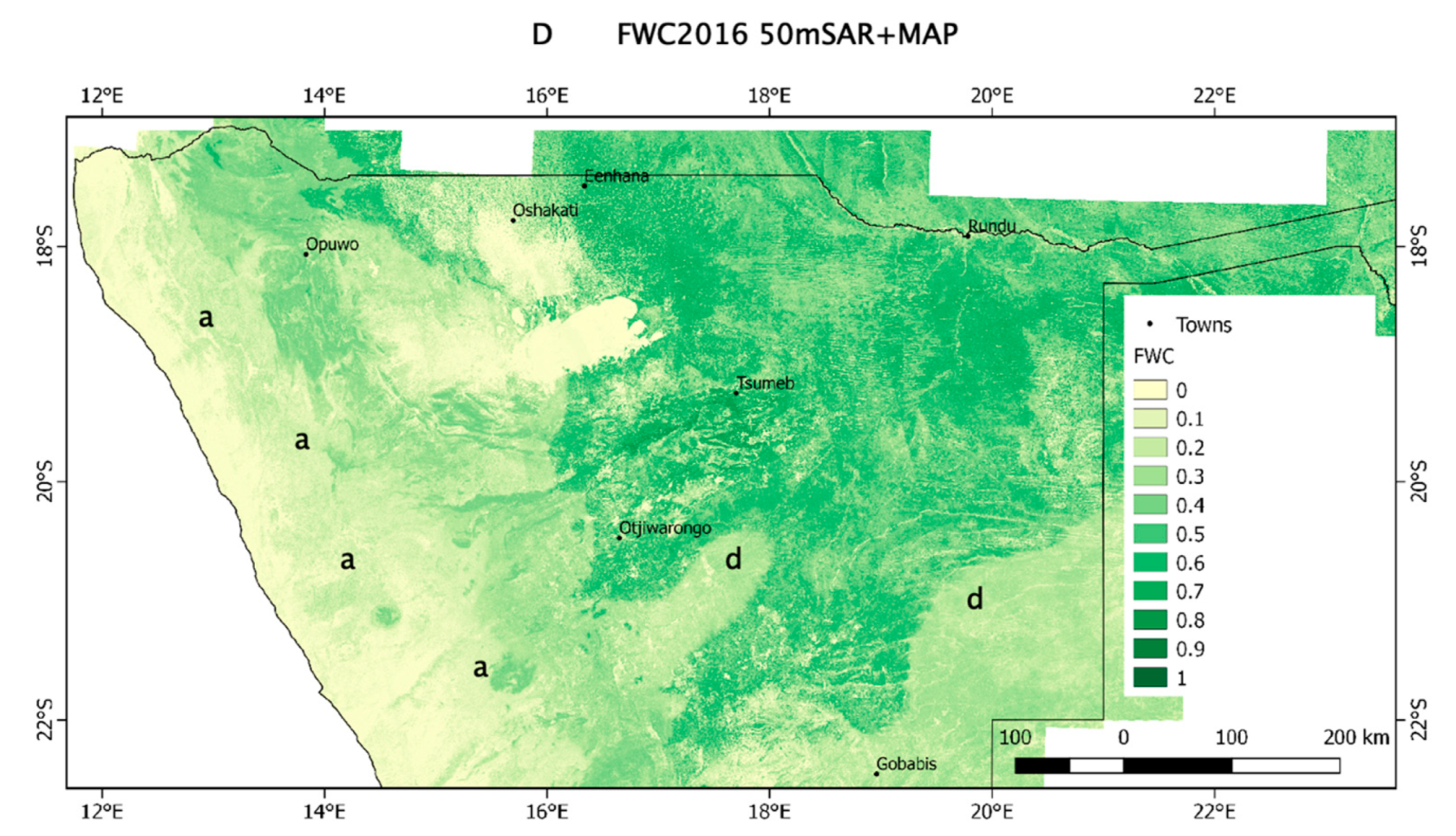
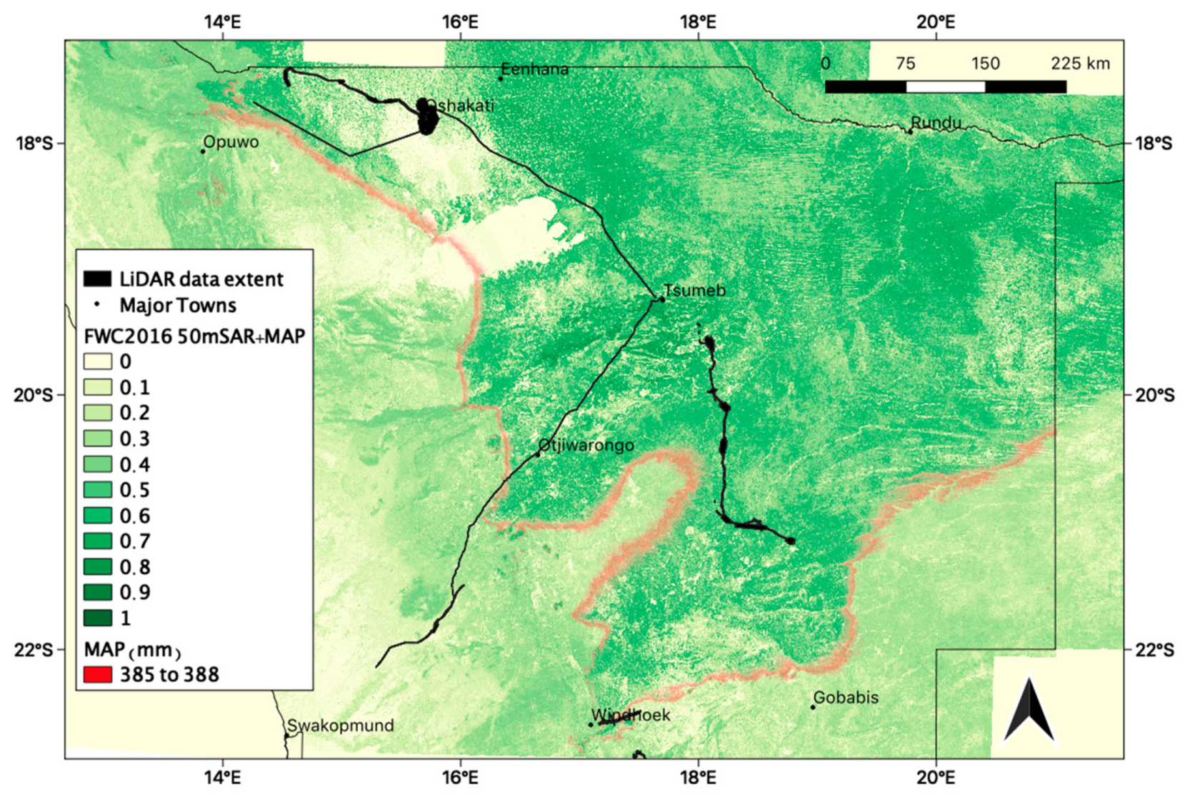
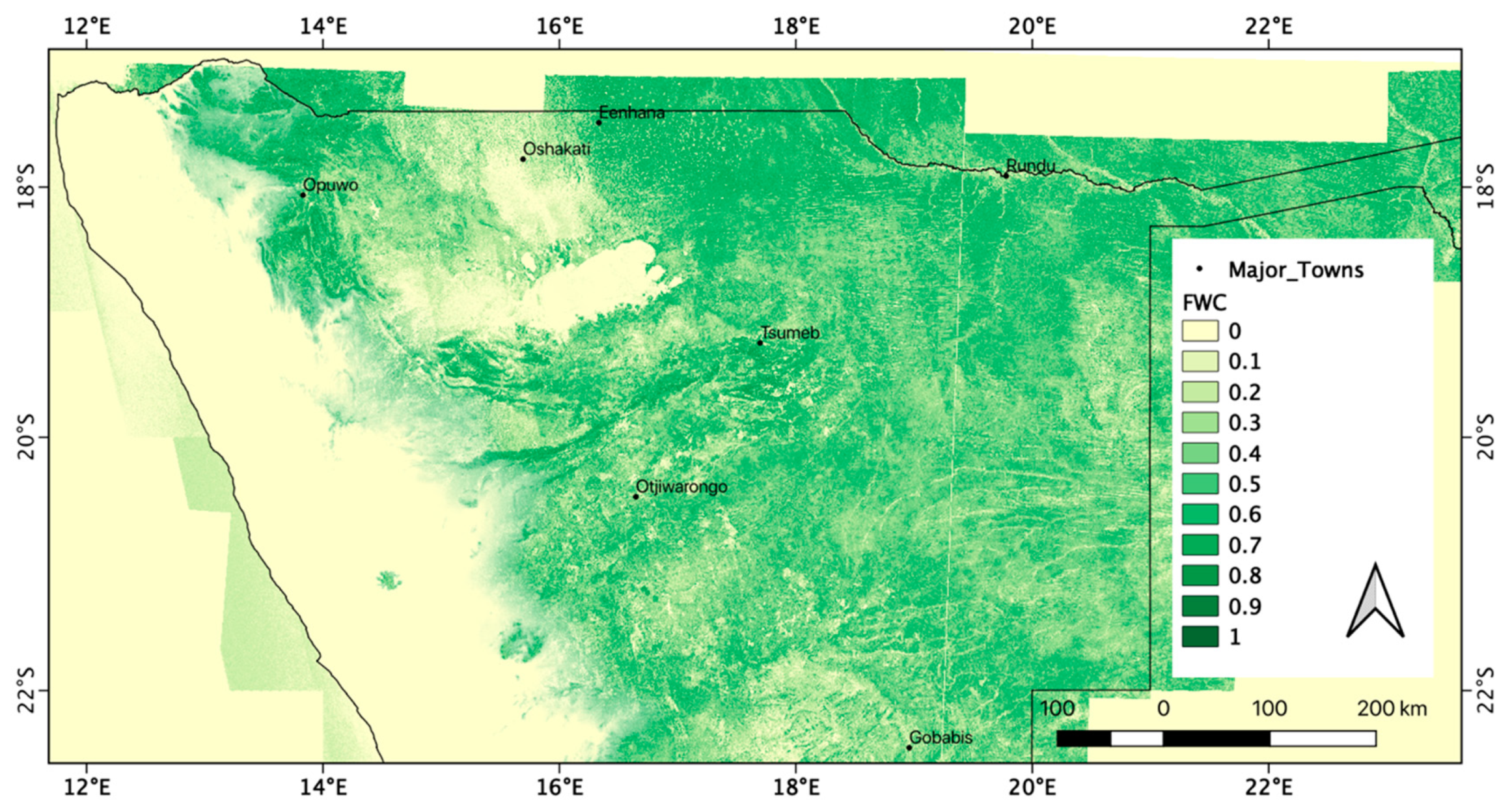
3.2. Regional Patterns of FWC Maps

The FWC map products differed significantly depending on the ancillary variable included i.e., elevation, MAP or both (Figure 7). Across all years, the FWC_50mSAR maps that did not include MAP or elevation, overestimated FWC in low rainfall areas (<250 mm) across the Namib Grasslands of the arid Western Highlands (Figure 1C and Figure 8A), especially in rocky areas with steep slopes which caused high backscatter (areas a in Figure 7A). The FWC_50mSAR+elev maps, underestimated FWC in the Caprivi region in the northeast of study area (areas b in Figure 7B,C). The FWC_50mSAR+elev maps also significantly overestimated FWC on steep slopes that caused high backscatter in the arid Namib Grasslands of the Western Highlands (100–250 mm) (areas a in Figure 7B). These contained sharp boundaries where FWC was overestimated above a specific local elevation threshold.

MAP is known to be a major determinant of woody cover in Africa [77]. To illustrate this relationship, the LiDAR FWC of the training data was graphed as a function of MAP (Figure S2). Except for a few outliers, MAP clearly set the upper limits for LiDAR FWC, for example, FWC largely remained below 0.5 where MAP was below 350 mm. However, within a specific MAP range, LiDAR FWC varied significantly below these upper bounds. Therefore, the inclusion of MAP (FWC_50mSAR+MAP) significantly reduced the overestimation of FWC in arid areas (areas a in Figure 7A vs. Figure 7D) and thus predicted more realistic FWC estimates (<0.5) in areas with MAP below 350 mm (Figure 8B). The FWC_50mSAR+MAP map provided the most realistic estimates in the Caprivi region (area b in Figure 7D, but contained a stark boundary in FWC corresponding to approximately 385–388 mm MAP (areas d in Figure 7D). Including both elevation and MAP as ancillary variables (FWC_{50mSAR+elev+MAP}) reduced contrast in FWC across the aforementioned rainfall-related anomaly, but reintroduced the stark boundary in FWC towards the Caprivi region (areas b in Figure 7C). The regional patterns and boundaries of these artifacts were consistent between years (not shown in the interest of brevity) suggesting that they were related to the static ancillary input data sets.

When comparing the histograms of the most recent map, (FWC2016_50mSAR+MAP) of the different vegetation structural classes (Figure 1C), FWC was very low in the Namib Grassland (mean = 0.05, SD = 0.05) and Dwarf Shrubland (mean = 0.08, SD = 0.12) and progressively increased within the Sparse Shrubland (mean = 0.18, SD = 0.11) and Grasslands (mean = 0.27, SD = 0.2) (Figure 9). It should be noted that the Grasslands structural class is not void of trees as the name suggests, but includes areas with a significant tree component such as the Omakatako drainage and the Caprivi Floodplains [54]. Dense Shrubland had a much higher FWC of 0.34 (SD = 0.16). The Shrubland–Woodland Mosaic class had a bimodal distribution with high frequencies at 0.2–0.3 and 0.5–0.6 FWC representing the shrubland and woodland patches, respectively [54]. The Woodland and Forest classes both had the highest FWC of 0.43 (SD = 0.15–0.16). The patches of forest are extremely small compared to the vast Woodland class (Figure 1C). The regional FWC patterns therefore conformed to the map of vegetation structural classes (Figure 9).

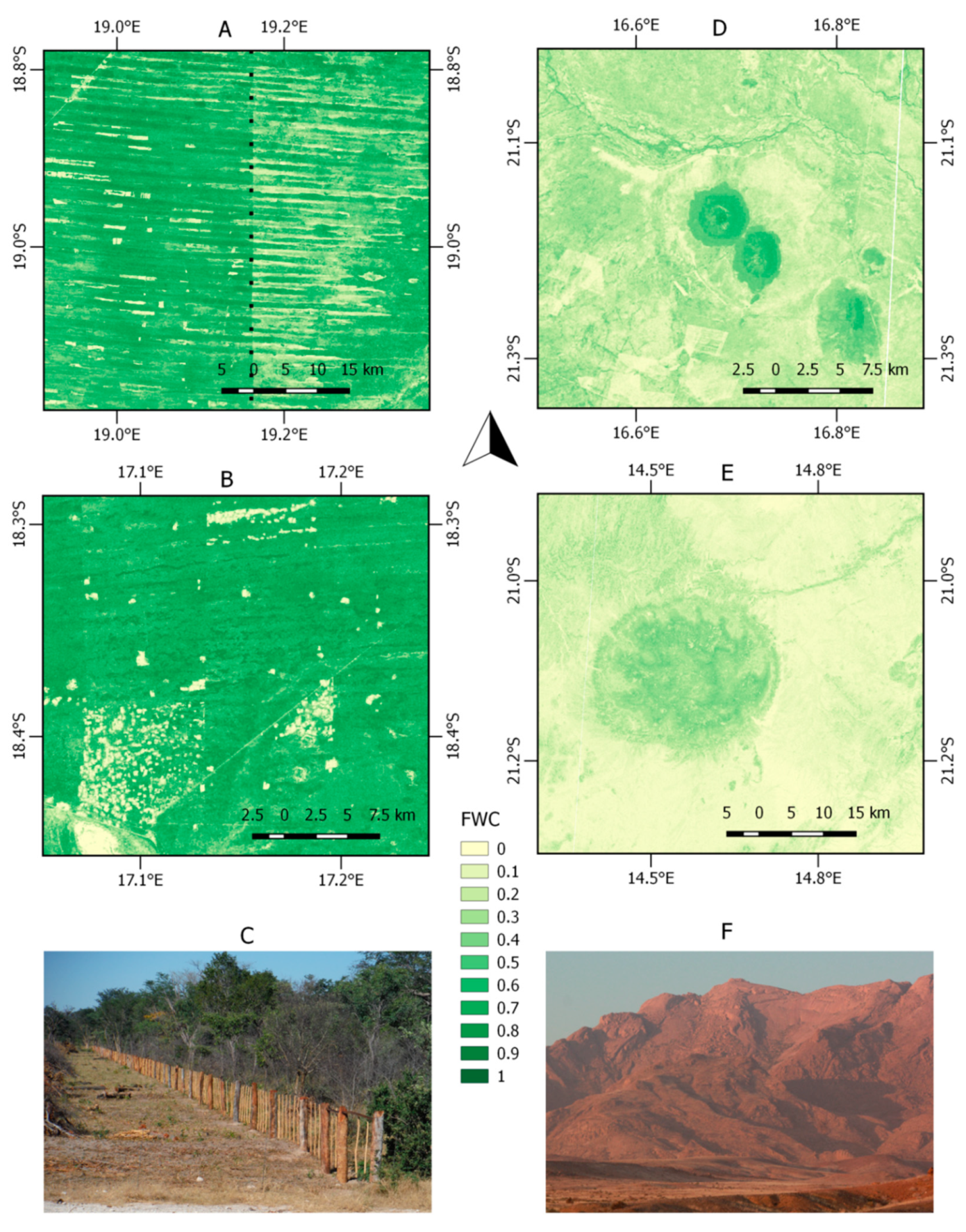
3.3. Local FWC Patterns

At a local scale, the FWC products contained substantial detail in the patterns of woody vegetation structure. The effect of the undulating sand dunes on the woody vegetation is clearly discernible with higher FWC on the crests and lower FWC in the troughs of the North-Eastern Kalahari Woodland (Figure 10A). Trees are often cleared for cultivated fields in the low-lying troughs of the dunes (Figure 10A,C). The impact of a veterinary fence on woody vegetation on the border of the Kavango district, was very pronounced, with 0.2–0.3 higher FWC on the western side of the fence (Foot-and-Mouth Disease Free zone) compared to the eastern side (Foot-and-Mouth Disease Buffer zone) (Figure 10A) [54]. This suggests that the long-term management and grazing differences on either side of the fence have led to significant differences in FWC.

Distinct patches of low FWC (<0.1) were caused by debushing for the production of charcoal in the dense (0.55–0.75 FWC) North-Eastern Kalahari Woodlands (Figure 10B). An overestimation of FWC was sometimes caused by high backscatter from the steep slopes (>20°) of the mountains and hills in arid areas, for example the Brandberg (Figure 10E,F) which has almost no woody cover on its rocky outcrops. This overestimation of FWC was however reduced by the inclusion of MAP as an ancillary variable. In other areas the drastic increase in FWC from the base towards the top of hills was correctly estimated by the FWC products and was not an anomaly caused by high backscatter from steep slopes (Figure 10D).

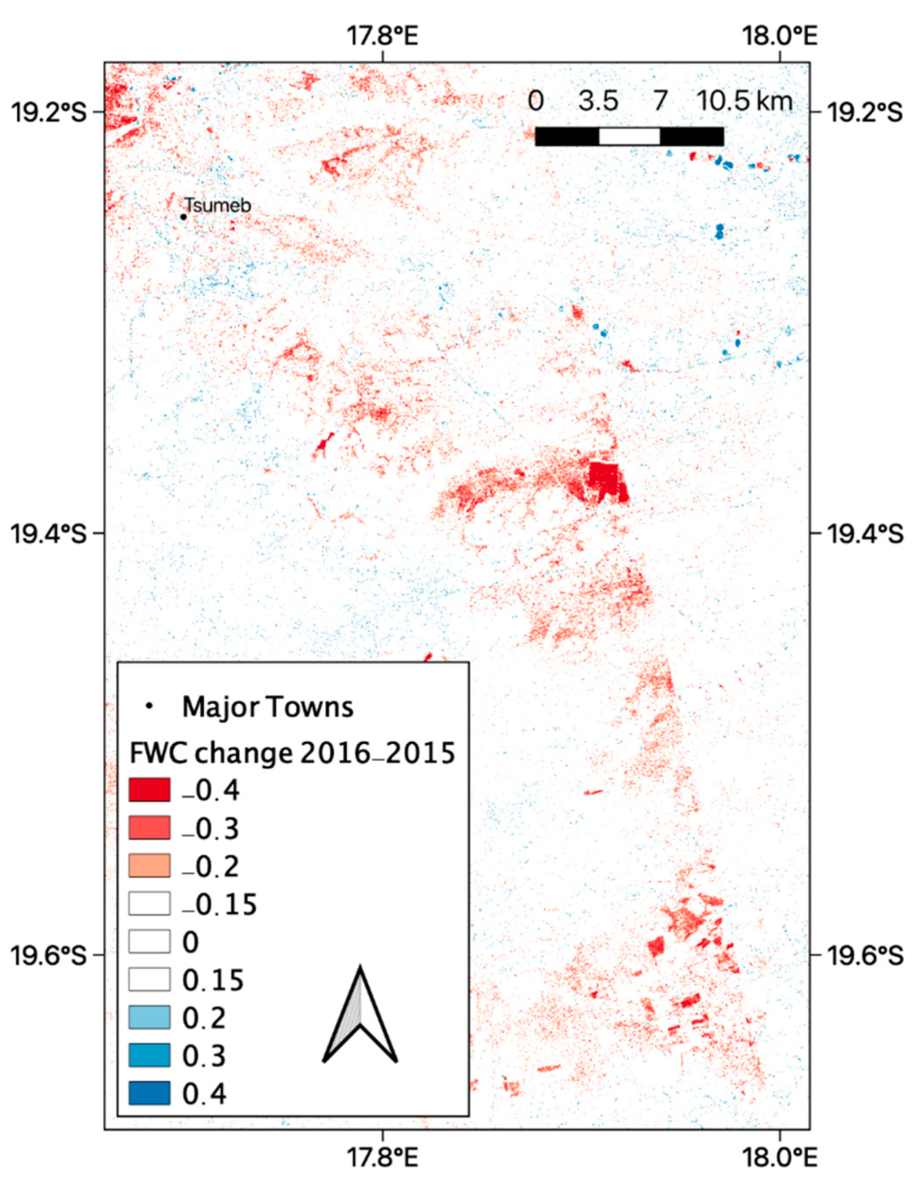
3.4. FWC Change Maps and Error Estimation

The uncertainty of a change products (e.g., σFWCΔ_2010–2009) was calculated from the RMSE’s of the annual FWC maps in Table 1

$${\sigma }_{FWC\mathsf{\Delta }2010-2009}=\sqrt{{0.12}^2+{0.12}^2}\approx 0.169$$

The change uncertainty σFWCΔ_2010–2009 of 0.169 represents the average uncertainty of all the individual pixels in the change product. The mean change uncertainty of all the pairs of years was 0.178 and ranged between 0.169 and 0.191. FWC change pixels of less than 0.15 were therefore excluded from all FWC maps and graphs in results below. All FWC change in the range of 0.15 to 0.20 were reported in results, but was considered unreliable and should be interpreted with caution. FWCΔ of more than 0.20 are considered to correspond to changes which were highly likely to have occurred on the ground.

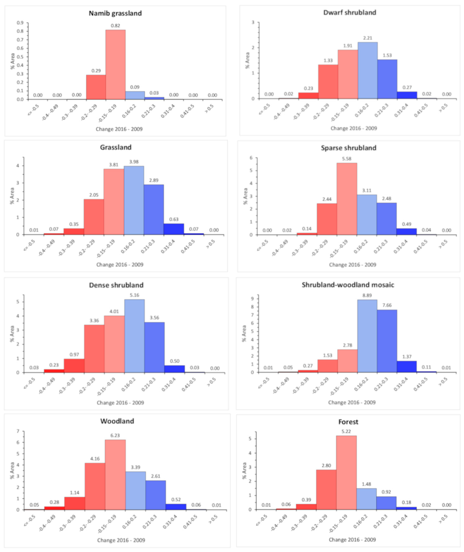
3.5. Regional FWC Change

The regional FWCΔ_2010–2009 and FWCΔ_2016–2015 was summarized for each vegetation structure class (Figures S3 and S4). When considering FWCΔ_2010–2009, an average of 98.7% of the area of the vegetation structural classes changed by less than 0.20. In general, the vegetation structural classes had equal areas which experienced more than 0.2 FWC increases and decreases across an average of 0.65% of their area. The following vegetation structural classes experienced the most change: Woodlands (1.25% decrease, 1.62% increase); Shrubland–Woodland Mosaic (1.28% decrease, 1.37% increase), Dense Shrubland (1.33% decrease, 1.37% increase), Grasslands (0.9% decrease, 1.76% increase). These low levels of change between successive years are credible. The percent areas change for FWCΔ_2016–2015 had very similar numbers compared to FWCΔ_2010–2009, suggesting that this monitoring approach does not produce highly variable and potentially erroneous FWC change between successive years (Figures S3 and S4).

When considering FWCΔ_2016–2009, an average of 95.8% of the area of the vegetation structural classes changed less than 0.20 (Figure 11). The areas affected by more than 0.2 FWC change across the seven-year study period, was three to five times larger per vegetation structural class than those which occurred between any two successive years (i.e., FWCΔ_2010–2009 and FWCΔ_2016–2015). The Namib grasslands contain extremely low levels of FWC and essentially contained no real or erroneous FWC change. In general, less than 4.5% of each vegetation structure class exhibited an increase or decrease in FWC of more than 0.20. The only exception was the Shrubland–Woodland Mosaic class which experienced increases in FWC > 0.20 across more than 9% of its area. The Sparse Shrublands and Dense Shrublands increased in FWC by 0.2–0.3 across 2.5% and 3.5% of their respective areas, while also decreasing in FWC by 0.2–0.3 across 1.8% and 2.97% of their respective areas. The FWC decreases of 0.3–0.4 that were typically caused by debushing (Section 3.6) was compared to increases in FWC of the same magnitude for each vegetation structure class. The Dense Shrubland had 1.9 times more area experiencing decreases in FWC of 0.3–0.4 than increases (0.97% vs. 0.5%) in FWC of the same magnitude. The Woodland class had double the area experiencing decreases of 0.3–0.4 than increases (1.14% vs. 0.52) (Figure 11). However, the Shrubland–Woodland Mosaic had six times more area experiencing increases in FWC of 0.3–0.4 than decreases (0.27% vs. 1.37).

At 50 m resolution the FWCΔ_2016–2009 map contained substantial “salt-and-pepper” effects that are difficult to visualize at regional scales. The regional patterns in FWCΔ_2016–2009 were therefore summarized as the mean of all 50 m pixels in a 20 km × 20 km grid (Figure 12). The mean FWCΔ values are lower than the values of the individual pixels. The most pronounced reductions in FWC (mean of −0.1 to −0.2) were concentrated around the town of Tsumeb in the center of the Woodlands structural class (Figure 12). The most pronounced increases in FWC (mean of 0.1 to 0.2) occurred in the central and south-eastern parts of the Shrubland–Woodland mosaic (mean of 0.1 to 0.2) and to a lesser extent in the central parts of the Dense Shrubland.

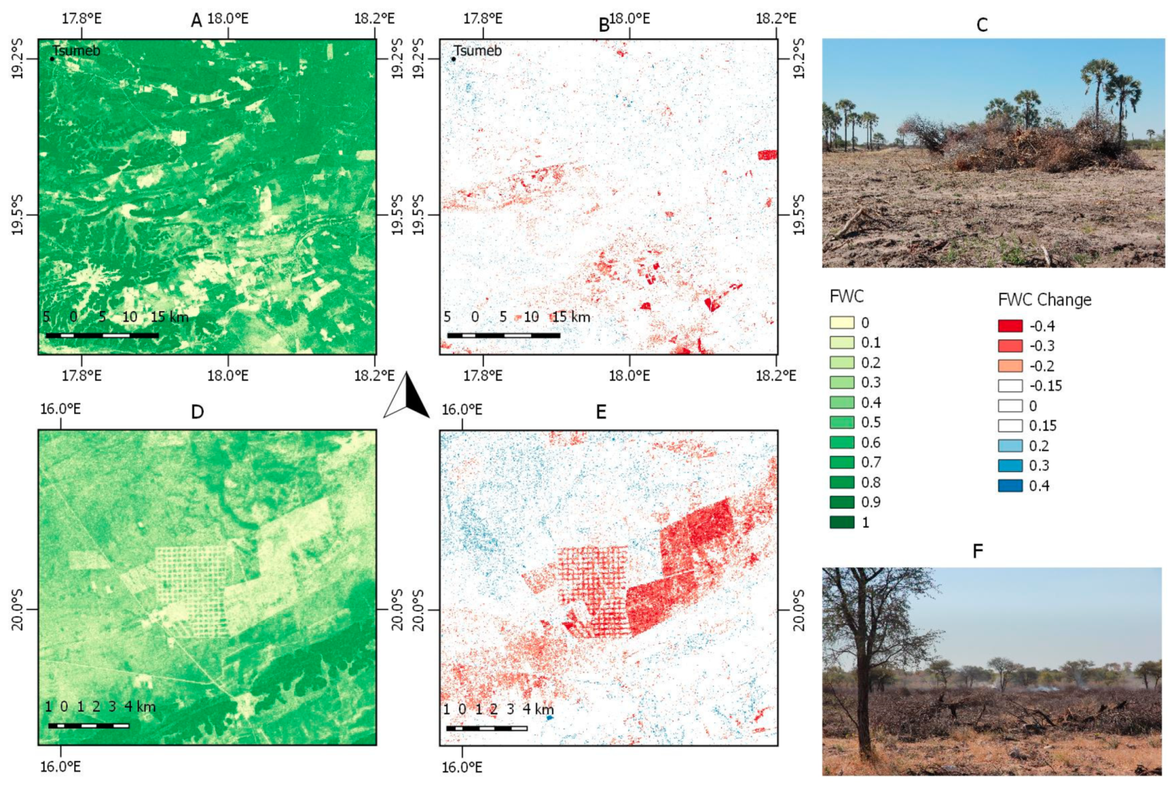
3.6. Local FWC Change Patterns

Sites of debushing by mechanical or chemical means were very effectively detected, especially in areas with high initial FWC which experienced a reduction of more than 0.3 FWC (Figure 13). Mechanical debushing often caused obvious change patterns which formed distinct geometric features of 300–3000 ha in size (3–30 km²) (Figure 13B,E, and Figure 14C). Grid patterns of debushing were clearly captured in the FWC change maps with reductions in FWC of more than 0.4 (Figure 13E). Debushing by means of poison applied in the field or from the air often caused lower FWC change and less distinctive features and boundaries in the change maps, as the trunks and branches of the dead, leafless trees and shrubs are often left standing for a few years after poisoning.

Increases in FWC often occurred in areas that were previously debushed, e.g., debushing in 2010–2009, followed by increase of 0.2–0.4 FWC between 2010 and 2016 (Figure 14C). In contrast to the rapid debushing which was easily identifiable at local scales, increases in FWC following debushing appeared to take place more gradually with lower FWC change magnitudes (Figure 14C). Increases in FWC of 0.2–0.3 also followed wildfires which significantly decreased the FWC in preceding years (Figure 14D–F).

4. Discussion

The study demonstrated the feasibility of scaling up an approach that was previous demonstrated in savannas at a local scale [52], to a national scale. Accordingly, we developed a system which uses large amounts of diverse airborne LiDAR data to train machine learning models to estimate FWC with ALOS PALSAR SAR data across vast areas. Although previous studies have demonstrated the approach of scaling up LiDAR to SAR estimates of forest structure using RF models, they focused on high biomass tropical forest [64,65,66,78]. The present study, on the other hand, is one of very few to implement this approach in arid and semi-arid savannas (150–650 mm rainfall) [51] and produced the first national-scale woody cover maps and change assessment derived from SAR data for Namibia. RF models are one of the most frequently used methods for mapping forest biomass with LiDAR or field plot training data and satellite data and its application in the present was justified by the large amount of available LiDAR data and the need to incorporate ancillary data sets [40,45,51,52,64,65,66,75].

Airborne LiDAR data provide an opportunity to use substantially larger sample sets to train models compared to approaches based on limited field plots [5]. To effectively use diverse LiDAR datasets of highly varying point density, we developed a novel method for processing LiDAR point cloud data to 1 m and 2 m CHMs that were then blended as a function of the LiDAR point density to produce an unbiased estimate of FWC for model training and validation. Without this blended approach the use of 1 m or 2 m CHMs would lead to over-or underestimation of LiDAR-derived FWC (Figure 3 and Figure 4) that would introduce large errors into the modeling approach from the outset. This technique allowed the efficient use of diverse LiDAR data sets [79].

At 50 m resolution, the average R² of the annual FWC_50mSAR maps was 0.65 (RSME = 0.16), but this improved notably with the addition of ancillary data, i.e., elevation: R² = 0.75 (RSME = 0.14), MAP: R² = 0.75 (RSME = 0.13) and both: R² = 0.79 (RSME = 0.12) (Table 1). The local studies in the Lowveld of South Africa, where our approach was first demonstrated, estimated FWC with R² = 0.77–0.80 (RMSE = 0.10–0.08) using only ALOS PALSAR backscatter as input and an output resolution of 105 m [45,52]. Scaling up this approach from a local study area of approximately 500 km² [45] to a study area that is a thousand times larger (500,000 km²), therefore resulted in slight to moderate increases in model uncertainty (FWC_50mSAR+MAP: R² = 0.75, FWC_50mSAR: R² = 0.65). Given that the FWC maps in the present study were furthermore produced at double the spatial resolution of the local studies (50 m vs. 105 m) [45,52], it suggests that the approach was successfully scaled up to national scales with an acceptable level of prediction error.

The addition of elevation and MAP as ancillary input datasets had a large influence on the R², RMSE, and the FWC patterns in the output map. Although the addition of elevation increased the R², the FWC_50mSAR+elev maps still contained overestimations of FWC in low rainfall areas and underestimations in the Caprivi region (Figure 7B). Improvements in R² with the addition of ancillary variable does therefore not necessarily lead to improved regional patterns in the FWC maps produced by the RF models. The addition of MAP as an ancillary variable reduced the overestimation of FWC in low rainfall areas (<250 mm) (Figure 1C and Figure 8A), especially in rocky areas with steep slopes which caused high SAR backscatter (area “a” in Figure 7A). The FWC_SAR+MAP maps did however contain artifacts in the form of sharp decreases in FWC in areas below approximately 387 mm MAP, leading to two clear discontinuities in the FWC products (Figure 15). This may be attributed to the specific geographic distribution of the LiDAR training data, which only includes one LiDAR data set that transcends the rainfall gradient to areas below 387 mm (Figure 15). This may have caused the RF model to create a sharp decision boundary when predicting FWC. Although the LiDAR data effectively sampled the limits of the environmental diversity of the study area, the shortage of LiDAR data in the region of 300–385 mm MAP and 1100–1400 m elevation most likely led to incorrect estimation of FWC in these areas (Figure 2). Similar studies in e.g., Panama, Asner et al. [64] had the opportunity to acquire LiDAR data that were systematically distributed over the entire country and the RF models did not produce any artifacts. In the current study the LiDAR data sets were arbitrarily located since the data were collected for other purposes. These data sets can however be augmented by additional LiDAR acquisitions targeting underrepresented environments (Figure 2). In the meantime the most prudent option would be to use the FWC_50mSAR map (Figure 6), which does not contain these obvious artifacts (albeit with slightly higher prediction error), while masking out hyper-arid areas with <200 mm MAP where there is very little woody cover or bush encroachment to be concerned about (Figure 16). The FWC maps produced for Namibia can provide baseline geospatial information for reporting and planning at national scales. The FWC maps contain substantially more detailed spatial information on woody vegetation structure than previous national maps on bush encroachment [19,53] or the vegetation structural map [54] (Figure 1) and can help inform policy on managing rangelands and woody resources [22,25,26].

All the models in the present study led to underestimations at high FWC and overestimations at low FWC (Figure 6), similar to the findings reported for other SAR-based estimations of woody biomass [78,80]. Although the saturation of L-band backscatter at biomass levels above 90–110 Mg ha⁻¹ is very well understood [70,81], it was not expected in these dryland savannas with biomass that is mostly below 60 Mg ha⁻¹ [51,82]. Several studies have however found these under and overestimations at opposite ends of multiple biomass ranges [66,83] and it has been attributed to properties of the RF regression, specifically, the averaging of predictions by an ensemble of individual trees which inevitably biases estimates to the sample mean [78,80]. This under-and over estimation of biomass is not, however, limited to RF models, but is a characteristic of all empirical methods that rely on ordinary least-squares regression (OLS). This well-established statistical phenomenon is referred to as regression dilution or bias dilution and is caused by error in the independent variable (e.g., field plot biomass or LiDAR-derived FWC) which biases the slope towards zero which results in under and over estimation of the dependent variable [84,85]. Alternatives to OLS, such as Reduced Major Axis regression and Theil–Sen slope estimator have been proposed for developing models estimating biophysical variables from remote sensing data [85].

The regional FWCΔ maps and their interpretation successfully addressed our objective of demonstrating the potential to monitor FWC change using SAR-derived maps. Interestingly, the locations of the above-mentioned artifacts in the FWC maps were consistent between years for any given combination of ancillary input data sets, allowing comparisons between years without leading to new artifacts in the FWCΔ products. The regional FWCΔ maps produced were realistic and showed credible changes within the seven-year period and less pronounced changes between sequential years (Figure 11 and Figures S3 and S4). The Dense Shrubland and Woodland classes appeared to experience a small net decrease in FWC due to mainly debushing activities. During the seven-year period the Shrubland–Woodland Mosaic was the only class that exhibited a regional net gain in FWC of more than 0.2 across 9% (11,906 km²) of its area that may potentially be attributed to bush encroachment (Figure 1C, Figure 11 and Figure 12). Unfortunately, no field data were available at a national or regional scale to validate this potential detected bush encroachment. However, given the limitations of change monitoring between only two points in time (e.g., 2016–2009) and the fact that bush encroachment is gradual process which manifests over decades [13,23,28], a more sophisticated time-series analysis approach (e.g., [86,87,88]) may be applied in the future to detect long-term trends in annual FWC derived from an extended ALOS PALSAR data record. Analysis of persistent, long-term trends will also address potential erroneous, tangential FWC change caused by surface moisture variability (discussed below).

At local scales, the individual FWC maps and the change maps clearly captured management impacts such as the difference in FWC caused by the veterinary fence and widespread debushing activities (Figure 13 and Figure 14). Although there are many change detection techniques for SAR data [89] that would have detected these changes, the approach presented here has the advantage of quantifying the change in units of FWC, which rangeland managers can easily interpret. Our findings of FWC change patterns were in line with those of Wingate et al. [51] who investigated woody biomass changes in the Kalahari Woodland vegetation type of Namibia [51] and found that woodland deforestation, degradation, thickening and regrowth (following deforestation) could be distinguished using ALOS PALSAR data (2005–2015). Distinct areas of debushing with decreases in FWC of more than 0.3 and area of 300–3000 ha (3–30 km²) were very effectively detected (Figure 13). Rapid woody vegetation regrowth, i.e., increases in FWC of 0.3–0.4 within six to seven years (2009–2016) following debushing activities, were also detected (Figure 14). This raises doubts around the effectiveness of costly debushing projects aimed at improving the animal production of rangelands, however it does lend support to the idea of sustainable harvesting for ongoing fuel production.

The use of free, annual ALOS PALSAR global mosaics presented a specific challenge. Areas of erroneous change in the FWC change product of 2016–2015 were caused by large differences in acquisition dates (313 days/11 months) of adjoining ALOS PALSAR strips used in the global mosaic of 2015. This resulted in contrasting surface moisture conditions between adjoining strips of the 2015 mosaic which caused differences of backscatter around 4–6 dB for HV and 6–8 dB for HH between the adjoining strips (Figure 17). This led to banding effects in the FWC of 2015, which was transferred to the FWCΔ_2016–2015 product, affecting 15,000 ha /150 km² (0.03% of study area). Although the banding anomaly affected only a small area, the effect of variable surface moisture may be present anywhere in the landscape, leading to less obvious, erroneous FWC change. The effect of contrasting surface moisture conditions on L-band SAR backscatter is very well documented [38] and can potentially be addressed by using only dry-season scenes acquired from May to October [43,49]. It may be possible to generate custom-made dry-season ALOS PALSAR mosaic for the region which would limit variability in surface moisture, however this would be more costly and would require substantially more frequent ALOS PALSAR acquisitions to fully address this problem [38,40]. Although the shorter C-band wavelength of the Sentinel1 sensor is less suited to monitoring woody vegetation structure than the longer L-band wavelength of ALOS PALSAR [39,43], the high temporal frequency (6–12 days) may help provide more data to derive backscatter composites with minimum surface moisture. This may potentially lead to FWC change products with fewer moisture-related artifacts while incurring only a slight increase in prediction error [72].

The processing of ALOS PALSAR global mosaics included the topographic normalization for variation in backscatter coefficient caused by slope [60]. However, the backscatter in the mosaics still increased sharply at slopes steeper than 20°, often in areas without any increase in tree cover, leading to overestimations of FWC (Figure 10E,F). Since steep terrain is not prevalent in the study area, a possible solution may have been to simply mask out areas with slopes > 20° from the FWC products. However, visual inspection revealed that on several hills the woody vegetation cover indeed increased sharply from the base towards the top of hills (Figure 10D). The relationship between FWC and slope therefore varied spatially in a complex manner. The inclusion of slope and aspect as ancillary input variables was tested to address this phenomenon, but their inclusion had no noticeable effect on FWC maps. Mapping woody biomass on steep slopes with SAR therefore remains a challenge [40].

5. Conclusions

The approach of mapping FWC with SAR data and RF models trained with large amounts of diverse, airborne LiDAR data was successfully scaled up to national scales with acceptable increases in model uncertainty compared to previous local studies (FWC_50mSAR: R² = 0.65, FWC_50mSAR+MAP: R² = 0.75 vs. R² = 0.77–0.80, RMSE = 0.10–0.08) [45,52]. This was one of the first studies to apply this approach at national scales in arid savannas and indeed the first attempt to produce SAR-derived FWC maps for Namibia. The FWC maps contain substantially more detailed spatial information on woody vegetation structure than existing national maps [19,53] (Figure 1A). The FWC maps that included MAP as ancillary variable had higher R², but the maps included anomalies in the form of sharp gradients in FWC along a MAP contour (387 mm). Therefore, although the LiDAR training data were expansive and sampled the limits of the data ranges, it was still spatially biased, leading to an anomalous decision boundary by the RF model. This could be addressed by a few supplementary airborne LiDAR data acquisitions targeted at underrepresented areas. At this point in time it is recommend that users use the FWC_50mSAR map (Figure 6) (which does not contain these artifacts), while masking out hyper-arid areas with <200 mm MAP where FWC is very low and in fact of limited management interest (Figure 16). The study successfully demonstrated the potential of SAR-derived FWC maps for monitoring woody vegetation change due to debushing and subsequent regrowth in low biomass, arid savannas. During the seven-year study period the Shrubland–Woodland Mosaic was the only vegetation structural class that exhibited a regional net gain in FWC of more than 0.2 across 9% (11,906 km²) of its area that may potentially be attributed to bush encroachment. The FWC change products may be used to assess of debushing programs and bush encroachment in relation to the objectives of Namibia’s national rangeland strategy and management programs [22,25,26]. This SAR-based approach is currently being applied and extended into a program by the Namibian Ministry of Agriculture, Water and Forestry and Germany’s GIZ to develop a national Bush Information System (BIS) to support farmers, charcoal industries, resource managers, and policy makers. The BIS has multiple aims, including mapping and quantifying bush encroachment, assessing woody biomass potential, and supporting the planning and monitoring of debushing activities.

References

1. Scholes, R.J.; Archer, S.R. Tree-Grass Interactions in Savannas. Annu. Rev. Ecol. Syst. 1997, 28, 517–544. [Google Scholar] [CrossRef]
2. Scholes, R. Savanna. In Vegetation of Southern Africa; Cowling, R.M., Richardson, D.M., Pierce, S.M., Eds.; Cambridge University Press: Cambridge, UK, 1997; pp. 258–277. [Google Scholar]
3. Sankaran, M.; Ratnam, J.; Hanan, N. Woody cover in African savannas: The role of resources, fire and herbivory. Glob. Ecol. Biogeogr. 2008, 17, 236–245. [Google Scholar] [CrossRef]
4. Hill, M.J.; Hanan, N.P. Ecosystem Function in Savannas: Measurement and Modeling at Landscape to Global Scales; CRC Press: Boca Raton, FL, USA; London, UK, 2010. [Google Scholar] [CrossRef]
5. Bouvet, A.; Mermoz, S.; Le Toan, T.; Villard, L.; Mathieu, R.; Naidoo, L.; Asner, G.P. An above-ground biomass map of African savannahs and woodlands at 25m resolution derived from ALOS PALSAR. Remote Sens. Environ. 2018, 206, 156–173. [Google Scholar] [CrossRef]
6. Adeel, Z.; Safriel, U.; Niemeijer, D.; White, R. Ecosystems and Human Well-Being: Desertification Synthesis; World Resources Institute (WRI): Washington, DC, USA, 2005. [Google Scholar]
7. Bond, W.J.; Midgley, G.F. A proposed CO2-controlled mechanism of woody plant invasion in grasslands and savannas. Glob. Chang. Biol. 2000, 6, 865–869. [Google Scholar] [CrossRef]
8. Wigley, B.J.; Bond, W.J.; Hoffman, M.T. Thicket expansion in a South African savanna under divergent land use: Local vs. global drivers? Glob. Chang. Biol. 2010, 16, 964–976. [Google Scholar] [CrossRef]
9. Bond, W.J.; Midgley, G.F. Carbon dioxide and the uneasy interactions of trees and savannah grasses. Philos. Trans. R. Soc. B-Biol. Sci. 2012, 367, 601–612. [Google Scholar] [CrossRef] [PubMed]
10. Buitenwerf, R.; Bond, W.J.; Stevens, N.; Trollope, W.S.W. Increased tree densities in South African savannas: >50 years of data suggests CO2 as a driver. Glob. Chang. Biol. 2012, 18, 675–684. [Google Scholar] [CrossRef]
11. Archer, E.R.M.; Landman, W.A.; Tadross, M.A.; Malherbe, J.; Weepener, H.; Maluleke, P.; Marumbwa, F.M. Understanding the evolution of the 2014–2016 summer rainfall seasons in southern Africa: Key lessons. Clim. Risk Manag. 2017, 16, 22–28. [Google Scholar] [CrossRef]
12. Archer, S. Tree-grass dynamics in a Prosopis-thornscrub savanna parkland: Reconstructing the past and predicting the future. Ecoscience 1995, 2, 83–99. [Google Scholar] [CrossRef]
13. O’Connor, T.G.; Puttick, J.R.; Hoffman, M.T. Bush encroachment in southern Africa: Changes and causes. Afr. J. Range Forage Sci. 2014, 31, 67–88. [Google Scholar] [CrossRef]
14. Rohde, R.F.; Hoffman, M.T. The historical ecology of Namibian rangelands: Vegetation change since 1876 in response to local and global drivers. Sci. Total Environ. 2012, 416, 276–288. [Google Scholar] [CrossRef] [PubMed]
15. Hoffmann, W.A.; Schroeder, W.; Jackson, R.B. Positive feedbacks of fire, climate, and vegetation and the conversion of tropical savanna. Geophys. Res. Lett. 2002, 29, 2052. [Google Scholar] [CrossRef]
16. Beerling, D.J.; Osborne, C.P. The origin of the savanna biome. Glob. Chang. Biol. 2006, 12, 2023–2031. [Google Scholar] [CrossRef]
17. Archer, S.; Boutton, T.W.; Hibbard, K.A. Trees in grasslands: Biogeochemical consequences of woody plant expansion. In Global Biogeochemical Cycles in the Climate System; Schulze, E.D., Harrison, S.P., Heimann, M., Holland, E.A., Lloyd, J., Prentice, I.C., Schimel, D., Eds.; Academic Press: San Diego, CA, USA, 2001; pp. 115–137. [Google Scholar]
18. Asner, G.P.; Elmore, A.J.; Olander, L.P.; Martin, R.E.; Harris, A.T. Grazing systems, ecosystem responses and global change. Annu. Rev. Environ. Resour. 2004, 29, 261–299. [Google Scholar] [CrossRef]
19. De Klerk, J. Bush Encroachment in Namibia: Report on Phase 1 of the Bush Encroachment Research, Monitoring, and Management Project; Ministry of Environment and Tourism, Directorate of Environmental Affairs: Windhoek, Namibia, 2004.
20. Ward, D. Do we understand the causes of bush encroachment in African savannas? Afr. J. Range Forage Sci. 2005, 22, 101–105. [Google Scholar] [CrossRef]
21. Joubert, D.F.; Rothauge, A.; Smit, G.N. A conceptual model of vegetation dynamics in the semiarid Highland savanna of Namibia, with particular reference to bush thickening by Acacia mellifera. J. Arid Environ. 2008, 72, 2201–2210. [Google Scholar] [CrossRef]
22. Stafford, W.; Birch, C.; Etter, H.; Blanchard, R.; Mudavanhu, S.; Angelstam, P.; Blignaut, J.; Ferreira, L.; Marais, C. The economics of landscape restoration: Benefits of controlling bush encroachment and invasive plant species in South Africa and Namibia. Ecosyst. Serv. 2017, 27, 193–202. [Google Scholar] [CrossRef]
23. Joubert, D.; Smit, G.; Hoffman, M. The influence of rainfall, competition and predation on seed production, germination and establishment of an encroaching Acacia in an arid Namibian savanna. J. Arid Environ. 2013, 91, 7–13. [Google Scholar] [CrossRef]
24. Bester, F. Major problem-bush species and densities in Namibia. Agricola 1999, 10, 1–3. [Google Scholar]
25. Ministry of Agriculture, Water and Forestry. Namibia Rangeland Management Policy and Strategy: Restoring Namibia’s Rangelands; Ministry of Agriculture, Water and Forestry: Windhoek, Namibia, 2012.
26. Rothauge, A. Baseline Assessment for the De-Bushing Programme in Namibia; Deutsche Gesellschaft für Internationale Zusammenarbeit (GIZ): Windhoek, Namibia, 2014. [Google Scholar]
27. Energy, W.E. Prefeasibility Study for Biomass Power Plant. Namibia: Biomass Supply Chain Management; Nampower: Windhoek, Namibia, 2012. [Google Scholar]
28. Stevens, N.; Erasmus, B.F.N.; Archibald, S.; Bond, W.J. Woody encroachment over 70 years in South African savannahs: Overgrazing, global change or extinction aftershock? Philos. Trans. R. Soc. B Biol. Sci. 2016, 371, 20150437. [Google Scholar] [CrossRef] [PubMed]
29. Hansen, M.C.; Potapov, P.V.; Moore, R.; Hancher, M.; Turubanova, S.A.; Tyukavina, A.; Thau, D.; Stehman, S.V.; Goetz, S.J.; Loveland, T.R.; et al. High-resolution global maps of 21st-century forest cover change. Science 2013, 342, 850–853. [Google Scholar] [CrossRef] [PubMed]
30. Sexton, J.O.; Noojipady, P.; Song, X.-P.; Feng, M.; Song, D.-X.; Kim, D.-H.; Anand, A.; Huang, C.; Channan, S.; Pimm, S.L.; et al. Conservation policy and the measurement of forests. Nat. Clim. Chang. 2015, 6, 192–196. [Google Scholar] [CrossRef]
31. Bastin, J.-F.; Berrahmouni, N.; Grainger, A.; Maniatis, D.; Mollicone, D.; Moore, R.; Patriarca, C.; Picard, N.; Sparrow, B.; Abraham, E.M.; et al. The extent of forest in dryland biomes. Science 2017, 356, 635–638. [Google Scholar] [CrossRef] [PubMed]
32. Tian, F.; Brandt, M.; Liu, Y.Y.; Rasmussen, K.; Fensholt, R. Mapping gains and losses in woody vegetation across global tropical drylands. Glob. Chang. Biol. 2017, 23, 1748–1760. [Google Scholar] [CrossRef] [PubMed]
33. Mitchard, E.T.; Flintrop, C.M. Woody encroachment and forest degradation in sub-Saharan Africa’s woodlands and savannas 1982–2006. Philos. Trans. R. Soc. B 2013, 368, 20120406. [Google Scholar] [CrossRef] [PubMed]
34. Skowno, A.L.; Thompson, M.W.; Hiestermann, J.; Ripley, B.; West, A.G.; Bond, W.J. Woodland expansion in South African grassy biomes based on satellite observations (1990–2013): General patterns and potential drivers. Glob. Chang. Biol. 2017, 23, 2358–2369. [Google Scholar] [CrossRef] [PubMed]
35. Wagenseil, H.; Samimi, C. Woody Vegetation Cover in Namibian Savannahs: A Modelling Approach Based on Remote Sensing (Die Gehölzdichte in den Savannen Namibias: eine fernerkundungsgestützte Modellierung). Erdkunde 2007, 61, 325–334. [Google Scholar] [CrossRef]
36. Tsalyuk, M.; Kelly, M.; Getz, W.M. Improving the prediction of African savanna vegetation variables using time series of MODIS products. ISPRS J. Photogramm. Remote Sens. 2017, 131, 77–91. [Google Scholar] [CrossRef] [PubMed]
37. Hall, F.G.; Bergen, K.; Blair, J.B.; Dubayah, R.; Houghton, R.; Hurtt, G.; Kellndorfer, J.; Lefsky, M.; Ranson, J.; Saatchi, S.; et al. Characterizing 3D vegetation structure from space: Mission requirements. Remote Sens. Environ. 2011, 115, 2753–2775. [Google Scholar] [CrossRef]
38. Lucas, R.; Armston, J.; Fairfax, R.; Fensham, R.; Accad, A.; Carreiras, J.; Kelley, J.; Bunting, P.; Clewley, D.; Bray, S.; et al. An Evaluation of the ALOS PALSAR L-Band Backscatter—Above Ground Biomass Relationship Queensland, Australia: Impacts of Surface Moisture Condition and Vegetation Structure. IEEE J. Sel. Top. Appl. Earth Obs. Remote Sens. 2010, 3, 576–593. [Google Scholar] [CrossRef]
39. Mitchard, E.T.A.; Saatchi, S.S.; Woodhouse, I.H.; Nangendo, G.; Ribeiro, N.S.; Williams, M.; Ryan, C.M.; Lewis, S.L.; Feldpausch, T.R.; Meir, P. Using satellite radar backscatter to predict above-ground woody biomass: A consistent relationship across four different African landscapes. Geophys. Res. Lett. 2009, 36, L23401. [Google Scholar] [CrossRef]
40. Cartus, O.; Kellndorfer, J.; Walker, W.; Franco, C.; Bishop, J.; Santos, L.; Fuentes, J. A National, Detailed Map of Forest Aboveground Carbon Stocks in Mexico. Remote Sens. 2014, 6, 5559–5588. [Google Scholar] [CrossRef] [Green Version]
41. Saatchi, S.; Marlier, M.; Chazdon, R.L.; Clark, D.B.; Russell, A.E. Impact of spatial variability of tropical forest structure on radar estimation of aboveground biomass. Remote Sens. Environ. 2011, 115, 2836–2849. [Google Scholar] [CrossRef]
42. Shimada, M.; Itoh, T.; Motooka, T.; Watanabe, M.; Shiraishi, T.; Thapa, R.; Lucas, R. New global forest/non-forest maps from ALOS PALSAR data (2007–2010). Remote Sens. Environ. 2014, 155, 13–31. [Google Scholar] [CrossRef]
43. Mathieu, R.; Naidoo, L.; Cho, M.A.; Leblon, B.; Main, R.; Wessels, K.; Asner, G.P.; Buckley, J.; Van Aardt, J.; Erasmus, B.F.; et al. Toward structural assessment of semi-arid African savannahs and woodlands: The potential of multitemporal polarimetric RADARSAT-2 fine beam images. Remote Sens. Environ. 2013, 138, 215–231. [Google Scholar] [CrossRef]
44. Mermoz, S.; Le Toan, T.; Villard, L.; Réjou-Méchain, M.; Seifert-Granzin, J. Biomass assessment in the Cameroon savanna using ALOS PALSAR data. Remote Sens. Environ. 2014, 155, 109–119. [Google Scholar] [CrossRef]
45. Naidoo, L.; Mathieu, R.; Main, R.; Kleynhans, W.; Wessels, K.; Asner, G.; Leblon, B. Savannah woody structure modelling and mapping using multi-frequency (X-, C-and L-band) Synthetic Aperture Radar data. ISPRS J. Photogramm. Remote Sens. 2015, 105, 234–250. [Google Scholar] [CrossRef] [Green Version]
46. Lucas, R.; Milne, A.; Cronin, N.; Witte, C.; Denham, R. The potential of synthetic aperture radar (SAR) for quantifying the biomass of Australia’s woodlands. Rangel. J. 2000, 22, 124–140. [Google Scholar] [CrossRef]
47. Lucas, R.M.; Cronin, N.; Lee, A.; Moghaddam, M.; Witte, C.; Tickle, P. Empirical relationships between AIRSAR backscatter and LiDAR-derived forest biomass, Queensland, Australia. Remote Sens. Environ. 2006, 100, 407–425. [Google Scholar] [CrossRef]
48. Lucas, R.M.; Moghaddam, M.; Cronin, N. Microwave scattering from mixed-species forests, Queensland, Australia. IEEE Trans. Geosci. Remote Sens. 2004, 42, 2142–2159. [Google Scholar] [CrossRef]
49. Urbazaev, M.; Thiel, C.; Mathieu, R.; Naidoo, L.; Levick, S.R.; Smit, I.P.J.; Asner, G.P.; Schmullius, C. Assessment of the mapping of fractional woody cover in southern African savannas using multi-temporal and polarimetric ALOS PALSAR L-band images. Remote Sens. Environ. 2015, 166, 138–153. [Google Scholar] [CrossRef] [Green Version]
50. Mitchard, E.T.A.; Saatchi, S.S.; Lewis, S.L.; Feldpausch, T.R.; Woodhouse, I.H.; Sonké, B.; Rowland, C.; Meir, P. Measuring biomass changes due to woody encroachment and deforestation/degradation in a forest–savanna boundary region of central Africa using multi-temporal L-band radar backscatter. Remote Sens Environ. 2011, 115, 2861–2873. [Google Scholar] [CrossRef] [Green Version]
51. Wingate, V.R.; Phinn, S.R.; Kuhn, N.; Scarth, P. Estimating aboveground woody biomass change in Kalahari woodland: Combining field, radar, and optical data sets. Int. J. Remote Sens. 2018, 39, 577–606. [Google Scholar] [CrossRef] [Green Version]
52. Naidoo, L.; Mathieu, R.; Main, R.; Wessels, K.; Asner, G.P. L-band Synthetic Aperture Radar imagery performs better than optical datasets at retrieving woody fractional cover in deciduous, dry savannahs. Int. J. Appl. Earth Obs. Geoinf. 2016, 52, 54–64. [Google Scholar] [CrossRef]
53. Bester, F.V. Bush encroachment -A thorny problem. In Namibia Environment; Tarr, P.W., Ed.; Directorate of Environmental Affairs, Ministry of Environment and Tourism: Windhoek, Namibia, 1996; Volume 1, pp. 175–177. [Google Scholar]
54. Mendelson, J.; Jarvis, A.; Roberts, C.; Robertson, T. Atlas of Namibia: A Portrait of the Land and Its People, 1st ed.; David Philip: Cape Town, South Africa, 2002. [Google Scholar]
55. Joubert, D.; Zimmermann, I.; Fendler, J.; Winschiers-Theophilus, H.; Graz, F.P.; Smit, N.; Hoffman, M.T. The development of an expert system for arid rangeland management in central Namibia with emphasis on bush thickening. Afr. J. Range Forage Sci. 2014, 31, 161–172. [Google Scholar] [CrossRef]
56. Fick, S.E.; Hijmans, R.J. WorldClim 2: New 1-km spatial resolution climate surfaces for global land areas. Int. J. Climatol. 2017, 37, 4302–4315. [Google Scholar] [CrossRef]
57. NASA Jet Propulsion Laboratory (JPL). NASA Shuttle Radar Topography Mission Global 1 Arc Second; v003, distributed by NASA EOSDIS Land Processes DAAC; NASA Jet Propulsion Laboratory (JPL): Sioux Falls, SD, USA, 2013. [CrossRef]
58. Shimada, M.; Itoh, T.; Motooka, T.; Watanabe, M.; Thapa, R. Generation of the first PALSAR-2 global mosaic 2014/2015 and change detection between 2007 and 2015 using the PALSAR and PALSAR-2. In Proceedings of the IEEE International Geoscience and Remote Sensing Symposium (IGARSS), Beijing, China, 10–15 July 2016; pp. 3871–3872. [Google Scholar]
59. Shimada, M.; Itoh, T.; Motooka, T. Regenerated ALOS-2/PALSAR-2 global mosaics 2016 and 2014/2015 for forest observations. In Proceedings of the IEEE International Geoscience and Remote Sensing Symposium (IGARSS), Fort Worth, TX, USA, 23–28 July 2017; pp. 2454–2457. [Google Scholar]
60. Small, D. Flattening gamma: Radiometric terrain correction for SAR imagery. IEEE Trans. Geosci. Remote Sens. 2011, 49, 3081–3093. [Google Scholar] [CrossRef]
61. Shimada, M.; Ohtaki, T. Generating large-scale high-quality SAR mosaic datasets: Application to PALSAR data for global monitoring. IEEE J. Sel. Top. Appl. Earth Obs. Remote Sens. 2010, 3, 637–656. [Google Scholar] [CrossRef]
62. Haralick, R.M. Glossary and index to remotely sensed image pattern recognition concepts. Pattern Recognit. 1973, 5, 391–403. [Google Scholar] [CrossRef]
63. Belgiu, M.; Drăguţ, L. Random forest in remote sensing: A review of applications and future directions. ISPRS J. Photogramm. Remote Sens. 2016, 114, 24–31. [Google Scholar] [CrossRef]
64. Asner, G.P.; Mascaro, J.; Anderson, C.; Knapp, D.E.; Martin, R.E.; Kennedy-Bowdoin, T.; van Breugel, M.; Davies, S.; Hall, J.S.; Muller-Landau, H.C.; et al. High-fidelity national carbon mapping for resource management and REDD+. Carbon Balance Manag. 2013, 8, 7. [Google Scholar] [CrossRef] [PubMed] [Green Version]
65. Mascaro, J.; Asner, G.P.; Knapp, D.E.; Kennedy-Bowdoin, T.; Martin, R.E.; Anderson, C.; Higgins, M.; Chadwick, K.D. A tale of two “forests”: Random Forest machine learning aids tropical forest carbon mapping. PLoS ONE 2014, 9, e85993. [Google Scholar] [CrossRef] [PubMed]
66. Urbazaev, M.; Thiel, C.; Cremer, F.; Dubayah, R.; Migliavacca, M.; Reichstein, M.; Schmullius, C. Estimation of forest aboveground biomass and uncertainties by integration of field measurements, airborne LiDAR, and SAR and optical satellite data in Mexico. Carbon Balance Manag. 2018, 13, 5. [Google Scholar] [CrossRef] [PubMed] [Green Version]
67. Fisher, J.T.; Witkowski, E.T.; Erasmus, B.F.; Mograbi, P.J.; Asner, G.P.; Aardt, J.A.; Wessels, K.J.; Mathieu, R. What lies beneath: Detecting sub-canopy changes in savanna woodlands using a three-dimensional classification method. Appl. Veg. Sci. 2015, 18, 528–540. [Google Scholar] [CrossRef] [Green Version]
68. Mograbi, P.J.; Asner, G.P.; Witkowski, E.T.; Erasmus, B.F.; Wessels, K.J.; Mathieu, R.; Vaughn, N.R. Humans and elephants as treefall drivers in African savannas. Ecography 2017, 40, 1274–1284. [Google Scholar] [CrossRef]
69. Russakoff, D.B.; Tomasi, C.; Rohlfing, T.; Maurer, C.R. Image similarity using mutual information of regions. In Proceedings of the European Conference on Computer Vision (ECCV2004), Prague, Czech Republic, 11–14 May 2004; pp. 596–607. [Google Scholar]
70. Yu, Y.; Saatchi, S. Sensitivity of L-band SAR backscatter to aboveground biomass of global forests. Remote Sens. 2016, 8, 522. [Google Scholar] [CrossRef] [Green Version]
71. Santoro, M.; Cartus, O. Research pathways of forest above-ground biomass estimation based on SAR backscatter and Interferometric SAR observations. Remote Sens. 2018, 10, 608. [Google Scholar] [CrossRef] [Green Version]
72. Main, R.; Mathieu, R.; Kleynhans, W.; Wessels, K.; Naidoo, L.; Asner, G. Hyper-Temporal C-Band SAR for Baseline Woody Structural Assessments in Deciduous Savannas. Remote Sens. 2016, 8, 661. [Google Scholar] [CrossRef] [Green Version]
73. Wessels, K.J.; Mathieu, R.; Erasmus, B.F.N.; Asner, G.P.; Smit, I.P.J.; van Aardt, J.A.N.; Main, R.; Fisher, J.; Marais, W.; Kennedy-Bowdoin, T.; et al. Impact of communal land use and conservation on woody vegetation structure in the Lowveld savannas of South Africa. For. Ecol. Manag. 2011, 261, 19–29. [Google Scholar] [CrossRef]
74. Breiman, L. Random forests. Mach. Learn. 2001, 45, 5–32. [Google Scholar] [CrossRef] [Green Version]
75. Baccini, A.; Asner, G.P. Improving pantropical forest carbon maps with airborne LiDAR sampling. Carbon Manag. 2013, 4, 591–600. [Google Scholar] [CrossRef] [Green Version]
76. Hall, M.; Frank, E.; Holmes, G.; Pfahringer, B.; Reutemann, P.; Witten, I.H. The WEKA Data Mining Software: An Update. ACM SIGKDD Explor. Newsl. 2009, 11, 10–18. [Google Scholar] [CrossRef]
77. Sankaran, M.; Hanan, N.P.; Scholes, R.J.; Ratnam, J.; Augustine, D.J.; Cade, B.S.; Gignoux, J.; Higgins, S.I.; Le Roux, X.; Ludwig, F.; et al. Determinants of woody cover in African savannas. Nature 2005, 438, 846–849. [Google Scholar] [CrossRef] [PubMed]
78. Xu, L.; Saatchi, S.S.; Yang, Y.; Yu, Y.; White, L. Performance of non-parametric algorithms for spatial mapping of tropical forest structure. Carbon Balance Manag. 2016, 11, 18. [Google Scholar] [CrossRef] [PubMed] [Green Version]
79. Naidoo, L. Quantifying the Structure of the Woody Element in Savannahs Using Integrated Optical and Synthetic Aperture Radar (SAR) Approach: A Stepping Stone towards Country Wide Monitoring in South Africa; University of Pretoria: Pretoria, South Africa, 2017. [Google Scholar]
80. Rodríguez-Veiga, P.; Quegan, S.; Carreiras, J.; Persson, H.J.; Fransson, J.E.; Hoscilo, A.; Ziółkowski, D.; Stereńczak, K.; Lohberger, S.; Stängel, M. Forest biomass retrieval approaches from earth observation in different biomes. Int. J. Appl. Earth Obs. Geoinf. 2019, 77, 53–68. [Google Scholar] [CrossRef]
81. Hensley, S.; Oveisgharan, S.; Saatchi, S.; Simard, M.; Ahmed, R.; Haddad, Z. An error model for biomass estimates derived from polarimetric radar backscatter. IEEE Trans. Geosci. Remote Sens. 2013, 52, 4065–4082. [Google Scholar] [CrossRef]
82. Wessels, K.J.; Colgan, M.S.; Erasmus, B.; Asner, G.; Twine, W.; Aardt, J.A.N.V.; Fisher, J.T.; Smit, I.P.J.; Mathieu, R. Unsustainable fuelwood extraction from South African savannas. Environ. Res. Lett. 2013, 8, 014007. [Google Scholar] [CrossRef]
83. Avitabile, V.; Herold, M.; Heuvelink, G.B.; Lewis, S.L.; Phillips, O.L.; Asner, G.P.; Armston, J.; Ashton, P.S.; Banin, L.; Bayol, N. An integrated pan-tropical biomass map using multiple reference datasets. Glob. Chang. Biol. 2016, 22, 1406–1420. [Google Scholar] [CrossRef] [PubMed] [Green Version]
84. Fuller, W.A. Measurement Error Models; John Wiley & Sons: New York, NY, USA, 2009; p. 440. [Google Scholar]
85. Rejou-Mechain, M.; Muller-Landau, H.C.; Detto, M.; Thomas, S.; Toan, T.L.; Saatchi, S.; Barreto-Silvia, J.; Bourg, N.; Bunyavejchewin, S.; Butt, N. Local spatial structure of forest biomass and its consequences for remote sensing of carbon stocks. Biogeosci. Discuss. 2014, 11, 5711. [Google Scholar] [CrossRef]
86. Wessels, K.J.; Prince, S.D.; Malherbe, J.; Small, J.; Frost, P.E.; VanZyl, D. Can human-induced land degradation be distinguished from the effects of rainfall variability? A case study in South Africa. J. Arid Environ. 2007, 68, 271–297. [Google Scholar] [CrossRef]
87. Wessels, K.J.; van den Bergh, F.; Scholes, R.J. Limits to detectability of land degradation by trend analysis of vegetation index data. Remote Sens. Environ. 2012, 125, 10–22. [Google Scholar] [CrossRef]
88. Verbesselt, J.; Hyndman, R.; Zeileis, A.; Culvenor, D. Phenological change detection while accounting for abrupt and gradual trends in satellite image time series. Remote Sens. Environ. 2010, 114, 2970–2980. [Google Scholar] [CrossRef] [Green Version]
89. Bovolo, F.; Bruzzone, L. The time variable in data fusion: A change detection perspective. IEEE Geosci. Remote Sens. Mag. 2015, 3, 8–26. [Google Scholar] [CrossRef]
Figure 1. Study area in northern Namibia (Inset). (A) Bush encroachment mapped as density of plants per hectare and species (after [19]), as well as LiDAR data extent (red). (B) Mean annual precipitation (MAP) (WorldClim v2) [56]. (C) Vegetation structural classes [54]. (D) Elevation [57].
Remotesensing 11 02633 g001
Figure 2. The elevation and MAP of samples of LiDAR training data (randomly sampled 500 m apart) and the study area (randomly sampled 2000 m apart). Please note that the color of data points is 50% transparent providing an indication of data density.
Remotesensing 11 02633 g002
Figure 3. (A) Density of LiDAR returns per m2 of typical LiDAR data set (south of Tsumeb) with highly variable point density. Fractional woody cover (FWC, 25 m resolution) derived from LiDAR using a CHM at 1 m (B), 2 m (C) ground sampling distance and using the blended model (D). White areas indicate no data.
Remotesensing 11 02633 g003
Figure 4. Percentage error of fractional woody cover calculated using 1 m canopy height model (CHM), 2 m CHM and blended model, in relation to LiDAR return density per 4 m2. (Note: 4 m2 was used as the area unit to better illustrate the effect of minor increases in the number of LiDAR returns).
Remotesensing 11 02633 g004
Figure 5. Diagram of operational processing system with components including explanatory input variables, training data generation from LiDAR data, random forest models, and outputs in the form of annual fractional woody cover maps.
Remotesensing 11 02633 g005
Figure 6. Difference between predicted FWC and LiDAR FWC per LiDAR FWC bin for 50 m resolution FWC maps (example for FWC200950mSAR+elev+MAP). Median, box: 25th and 75th percentiles = interquartile range (IQR), whiskers: quartile ±1.5*IQR.
Remotesensing 11 02633 g006
Figure 7. Fractional woody cover of northern Namibia estimated using ALOS PALSAR SAR data Figure 2016 and specified ancillary input datasets: (A) no ancillary data, (B) elevation, (C) elevation and MAP, and (D) MAP. Lower case letters on maps indicate areas with specific anomalies that are discussed in the text.
Remotesensing 11 02633 g007aRemotesensing 11 02633 g007b
Figure 8. Density plot of mean annual precipitation (MAP) and fractional woody cover (FWC) predicted by random forest models including, (A) SAR only (no ancillary variables), (B) MAP, and (C) elevation and MAP.
Remotesensing 11 02633 g008
Figure 9. Histograms of fractional woody cover (FWC) within dominant vegetation structure classes (Figure 1C) based on FWC201650mSAR+MAP.
Remotesensing 11 02633 g009
Figure 10. Examples of local fractional woody cover maps (FWC201050mSAR+MAP). (A) Undulating patterns of FWC (south to north) caused by dunes in the North-Eastern Kalahari Woodlands. Fence-line contrast in FWC on both sides (west vs. east) of a foot-and-mouth disease veterinary fence (dashed line). (B) Very high FWC near the town of Oshivelo in the North-Eastern Kalahari Woodlands displaying distinct patches of debushing for charcoal production. (C) Debushing for charcoal production and subsistence cultivation. (D) Correct estimation of FWC on steep slopes of hills south of Otjiwarongo. (E) Overestimation of FWC on steep, barren slopes of (F) the Brandberg.
Remotesensing 11 02633 g010
Figure 11. Changes in fractional woody cover between 2016 and 2009 for each vegetation structural class. Changes of less than 0.15 fractional woody cover were excluded as this was less than the average change uncertainty, σFWCΔ.
Remotesensing 11 02633 g011
Figure 12. Mean fractional woody cover change (2016–2009) within 20 km × 20 km grid cells overlaid with three dominant structural vegetation classes (hatching).
Remotesensing 11 02633 g012
Figure 13. Examples of local patterns of fractional woody cover change maps (FWC Change, 50 m resolution). (A) Fractional woody cover of Tsumeb area in 2010 (FWC201050mSAR+MAP) and (B) the corresponding FWCΔ2010–2009 showing distinct areas of debushing activities (FWC change > −0.3). (D) FWC of area north of the town of Outjo in 2016 (FWC201650mSAR+MAP) which experienced (E) significant changes in FWC since 2009 (FWCΔ2016–2009) due to debushing activities in a grid pattern. (C,F) Examples of mechanical debushing in the field.
Remotesensing 11 02633 g013
Figure 14. Examples of local patterns of fractional woody cover change maps. (A) FWC200950mSAR+MAP of area south of Tsumeb area in 2009 and (B) FWC201650mSAR+MAP. (C) Corresponding FWCΔ2016–2009 showing distinct areas of debushing (FWCΔ < −0.3) and areas where FWC has increased (FWCΔ > 0.2), following debushing prior to 2009. (D) FWC of area north of Gobabis where a wildfire reduced the FWC in 2009 after which the area experienced an increase in FWC up to 2016 (E,F).
Remotesensing 11 02633 g014
Figure 15. Artifact in FWC maps (e.g., FWC201650mSAR+MAP) causing a sharp change in FWC corresponding to 385–388 mm mean annual precipitation (MAP) band. The extent of the airborne LiDAR data using as training data (black).
Remotesensing 11 02633 g015
Figure 16. Fraction woody cover derived using only SAR variables (FWC201650mSAR), with a mask applied over areas with MAP < 200 mm.
Remotesensing 11 02633 g016
Figure 17. FWCΔ2016–2015 displaying a banding anomaly caused by contrasting surface moisture conditions and resulting backscatter in adjacent strips of 2015 ALOS PALSAR global mosaic.
Remotesensing 11 02633 g017