Estimating Spatio-Temporal Variations of PM_2.5 Concentrations Using VIIRS-Derived AOD in the Guanzhong Basin, China

Abstract

Aerosol optical depth (AOD) derived from satellite remote sensing is widely used to estimate surface PM_2.5 (dry mass concentration of particles with an in situ aerodynamic diameter smaller than 2.5 µm) concentrations. In this research, a two-stage spatio-temporal statistical model for estimating daily surface PM_2.5 concentrations in the Guanzhong Basin of China is proposed, using 6 km × 6 km AOD data available from the Visible Infrared Imaging Radiometer Suite (VIIRS) instrument as the main variable and meteorological factors, land-cover, and population data as auxiliary variables. The model is validated using a cross-validation method. The linear mixed effects (LME) model used in the first stage could be improved by using a geographically weighted regression (GWR) model or the generalized additive model (GAM) in the second stage, and the predictive capability of the GWR model is better than that of GAM. The two-stage spatio-temporal statistical model of LME and GWR successfully captures the temporal and spatial variations. The coefficient of determination (R²), the bias and the root-mean-squared prediction errors (RMSEs) of the model fitting to the two-stage spatio-temporal models of LME and GWR were 0.802, −0.378 µg/m³, and 12.746 µg/m³, respectively, and the model cross-validation results were 0.703, 1.451 µg/m³, and 15.731 µg/m³, respectively. The model prediction maps show that the topography has a strong influence on the spatial distribution of the PM_2.5 concentrations in the Guanzhong Basin, and PM_2.5 concentrations vary with the seasons. This method can provide reliable PM_2.5 predictions to reduce the bias of exposure assessment in air pollution and health research.

1. Introduction

Ambient air pollution is associated with human health and, thus, considered as a public health concern worldwide [1,2]. Particulate matter is an important component of air pollution. PM_2.5 (the integrated mass concentration of fine particulate matter with aerodynamic diameter less than or equal to 2.5 µm) is used as a measure of the health-related aerosol mass concentration. High concentrations of PM_2.5 occur in regions across the world [3] with strong contributions from anthropogenic emissions, biomass burning aerosols, and desert dust, augmented by meteorological conditions conducive for the formation of haze (e.g., References [4,5]). Where anthropogenic emissions occur in certain regions with much industrial activity, traffic, urbanization, etc., and little emission control, such as some developed countries and developing countries like India and China, biomass burning activities such as forest fires and agricultural burning are seasonal and may contribute strongly to the local and reginal air pollution (e.g., Reference [6]). Desert dust aerosol is generated during dust storms and can be transported over long distances. Dust particles have large size (> 1 µm) and, thus, have a relatively large mass, and desert dust aerosol contributes to 30% to 35% of the total mass of aerosols emitted into the atmosphere every year [7]. Exposure to desert dust PM_2.5 is estimated to lead to the premature death of 3.56 million people each year [8]. Dust pollution is a serious environmental issue, e.g., in the Atlantic [9], Carpathian Basin (central Europe) [10], Fuerteventura (Canary Islands) [11], Delhi, India [12], and southeast China [13].

As a result of the acceleration of economic development and urbanization in China, the energy consumption and the emission of various air pollutants increased. Air pollution in China is a serious problem, with pollutant concentrations among the highest in the world, especially with regard to particulate matter [3,14,15] and ground-based PM_2.5 [16,17]. A large number of epidemiological studies showed that PM_2.5 is related to a series of diseases [18,19]. PM_2.5 particles can be inhaled deep into the lungs, affecting lung function and causing respiratory and cardiovascular diseases, and they may even result in premature death [20,21]. The World Health Organization (WHO) reported 4.2 million premature deaths worldwide per year in 2016 (https://www.who.int/news-room/fact-sheets/detail/ambient-(outdoor)-air-quality-and-health, last access 1 November 2019). Even short-term exposure to high concentrations of PM_2.5 may have serious adverse effects on human health [22], and it was identified as the fourth major risk factor for mortality in China [23]. Long-term and large-scale monitoring of the PM_2.5 spatio-temporal distribution characteristics is crucial to assessing aerosol effects on public health. However, a national PM_2.5 monitoring network was established in China only by the end of 2012 [16], and, before that, no surface PM_2.5 data were available in many areas. This limits an accurate assessment of the effects of PM_2.5 on health.

Aerosol optical depth (AOD) is the integral of the aerosol extinction coefficient over the whole vertical column in the atmosphere and can be retrieved over large spatial scales from satellite data (e.g., Reference [24]). AOD describes the attenuation of incoming solar radiation in the atmosphere due to aerosol particles by scattering and absorption. It can be used as a proxy for the concentration of particulate matter in the atmospheric column and the degree of air pollution. Therefore, monitoring of PM_2.5 concentrations based on satellite-derived AOD data was widely attempted complementary to ground-based in situ measurements, to obtain a large spatial coverage [16,17,25,26,27,28]. However, the PM_2.5/AOD relationship depends on a multitude of factors. Research on the PM_2.5/AOD relationship in China was mainly concentrated in the Beijing–Tianjin–Hebei area [29], the Pearl River Delta and the Yangtze River Delta area [30], and all of China [16,28]. The air quality in the Guanzhong Basin urban agglomeration with Xi’an as the major city is affected by natural conditions (such as topography and meteorology, as well as the transport of dust) and anthropogenic factors (such as industrial, household, and traffic emissions), resulting in frequent exceedance of the air quality standards. The Guanzhong Basin is one of the most polluted areas in China [31,32], but very few studies on air quality and pollution levels were carried out in this area. The goal of the current study was to develop a method, using satellite data, to systematically study PM_2.5 concentrations and obtain the spatio-temporal characteristics of air pollution in the Guanzhong Basin area, complementary to the sparsely distributed PM_2.5 ground-based monitoring stations.

In the existing literature, three main methods were reported to obtain surface PM_2.5 concentrations from satellite-retrieved AOD data. The proportional factor method is based on the use of satellite-retrieved AOD together with a chemical transport model (CTM) [2,3]. The physical-based method uses semi-empirical formulas describing the relationship between PM_2.5 and AOD based on physical processes [33,34]. The statistical method involves a simple linear regression method [35] or a generalized linear regression model [36]. In order to reflect the non-linear relationship between PM_2.5 and AOD more accurately, complex advanced models were developed to relate PM_2.5 concentrations to AOD through meteorological parameters (e.g., temperature, boundary layer height, relative humidity, and wind speed). Examples are the generalized additive model [26], linear mixed effect model [1,28,37], geographically weighted regression model [29,38], nested linear mixed effects model [39], random forest machine learning models [40,41], and spatial backpropagation neural network method [42]. However, these models may not completely capture the complex spatio-temporal relationship between PM_2.5 and prediction factors. In this study, we developed a geographically weighted regression model, constrained by satellite observations of AOD, which revealed the temporal and spatial variations of PM_2.5 in the research area. In addition, we also used the generalized additive model to ensure the spatial continuity of the relationship between PM_2.5 and AOD, and we compared it with the geographically weighted regression model developed.

Previous studies mainly used AOD data retrieved from the Moderate Resolution Imaging Spectroradiometer (MODIS) or the Multiangle Imaging Spectroradiometer (MISR) to estimate surface PM_2.5 concentrations. However, the nominal spatial resolutions of the AOD available as MODIS and MISR operational products are relatively coarse: 10 km × 10 km and 17.6 km × 17.6 km, respectively [38]. The successor of MODIS is the Visible Infrared Imaging Radiometer Suite (VIIRS) launched by the United States National Aeronautics and Space Administration (NASA) on the Suomi National Polar-orbiting Partnership (S-NPP) satellite on 28 October 2011. VIIRS provides aerosol products based on the MODIS heritage (https://www.star.nesdis.noaa.gov/smcd/spb/aq/subs/docs/VIIRS_Aerosol_Product_Description.pdf, last access 1 November 2019). The retrieval inherits the MODIS dark target (DT) algorithm and takes into account a series of characteristics of the VIIRS sensor, such as the spectral response and spatial resolution, in order to meet the needs of global observation after MODIS retirement [43]. Exploring the performance of VIIRS AOD to estimate PM_2.5 over the Guanzhong area was also a purpose of our research.

The objective of this analysis was to establish a model, using VIIRS AOD data, meteorological data, land-use information, and population data, which provide the spatial and temporal relationship between PM_2.5 and AOD, and use this model to estimate PM_2.5 concentrations in the Guanzhong area. Temporal and spatial distributions of predicted surface PM_2.5 were then derived from the model to illustrate the variations of ground-level PM_2.5 concentrations within the study area.

2. Materials and Methods

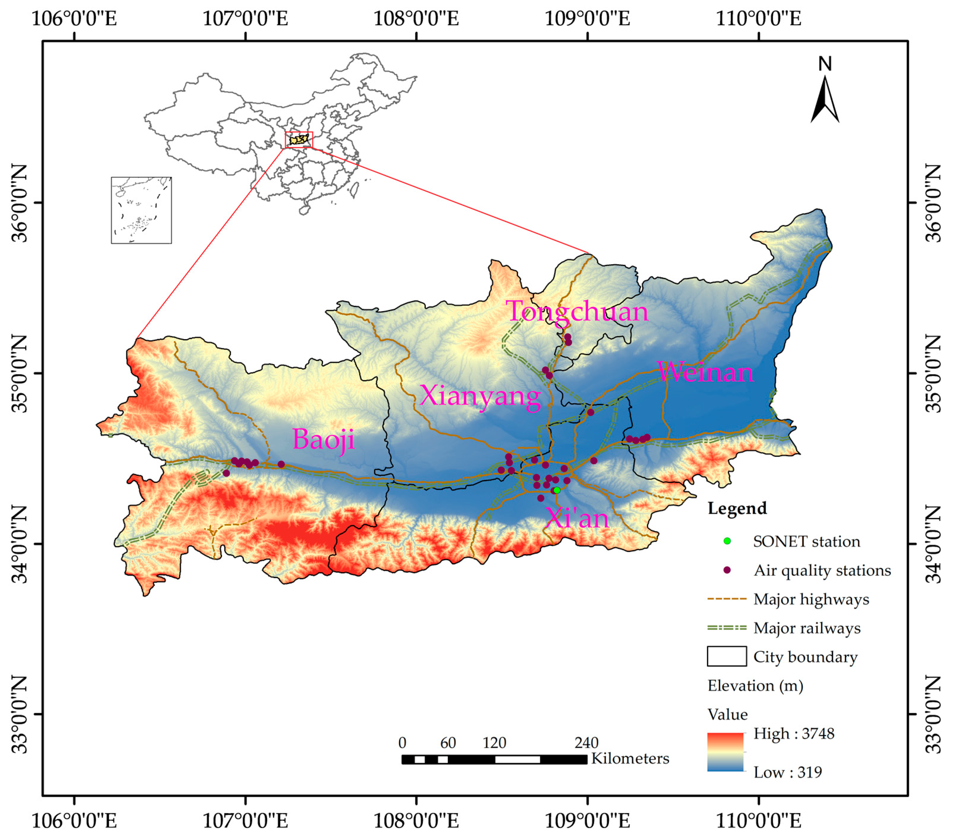
2.1. Study Area

The Guanzhong Basin is located in the central part of the Shaanxi Province (China). The Basin mainly includes plains and part of the Loess Plateau with five cities, Xi’an, Xianyang, Weinan, Tongchuan, and Baoji, as shown in Figure 1. It is narrow in the west and wide in the east and covers an area of around 55,600 km². The Guanzhong area has a unique trumpet-shaped basin enclosed between the Loess Plateau in the north and the Qinling Mountains in the south. The topography of the basin surrounded by mountains and the plateau limits the transport of pollutants out of the area; in particular, when wind speed is low, the concentrations can be very high. In episodes with dry weather and low wind speed, industrial emissions could also increase the degree of environmental pollution. Due to the dense population and developed economy, the annual motor vehicle exhaust and the coal combustion and biomass burning in the winter are also major contributions to the PM_2.5 concentrations in the area. The three main ions of PM_2.5 in Xi’an (the core city of Guanzhong area) are sulfate, nitrate, and ammonium [44]. Much of the PM_2.5 in the atmosphere over Xi’an is produced by anthropogenic activities [45]. In addition, sand and dust generated over the Loess Plateau, as well as dust from the Gurbantunggut Desert, Taklimakan Desert, and Badain Jaran Desert, are transported to the Guanzhong Basin by the prevailing northerly Asian winter monsoonal winds, which could also aggravate the pollution in the study area [46].

2.2. Data Collection

2.2.1. Ground-Based PM_2.5 Concentration Data

Hourly PM_2.5 concentration data for the major cities in all provinces of China are made available to the public by the environment ministry of China Environmental Monitoring Center (CNEMC) since 2012 [16]. As shown in Figure 1, there are 33 air quality monitoring stations in the Guanzhong area, each of which provides hourly mean PM_2.5 concentrations (µg/m³). These monitoring stations are located in five cities, i.e., 13 stations in Xi’an, four in Xianyang, four in Weinan, four in Tongchuan, and eight in Baoji. Only seven of these monitoring stations are located in suburban or rural areas. Following the Chinese directives for ambient air quality standards, the ground-based PM_2.5 concentrations are measured by a tapered element oscillating microbalance (TEOM) or a beta-ray with monthly data quality calibration and controlled processing (http://kjs.mee.gov.cn/hjbhbz/bzwb/jcffbz/201109/W020120130460791166784.pdf, last access 1 November 2019). For the current study, we collected ground-based PM_2.5 concentrations averaged between 1:00 and 2:00 p.m. local time (LT) at 33 stations in the Guanzhong area, for the period from 1 January to 31 December 2017, from the website of the CNEMC (http://113.108.142.147:20035/). The time slot between 1:00 and 2:00 p.m. LT was selected to match the NPP satellite overpass time at 1:30 p.m. (LT). Invalid data due to equipment breakdown (values recorded as not available (NA)) were removed from the dataset before it was used in our study.

2.2.2. Satellite-Retrieved AOD Products

The S-NPP satellite was launched on 28 October 2011. It is the new generation of the National Polar-orbiting Operational Environmental Satellite System Preparatory Project in the United States. NPP carries five earth observation instruments including VIIRS [47]. VIIRS is a cross-track scanning radiometer that extends and improves the data series collected from the Advanced Very-High-Resolution Radiometer (AVHRR) launched by the National Oceanic and Atmospheric Administration (NOAA) and MODIS launched by NASA.

VIIRS has a swath width of 3060 km, providing daily global coverage with a spatial resolution that depends on the spectral band. Out of 22 spectral bands, 16 have moderate spatial resolution of 750 m at nadir with wavelengths between 0.412 µm and 12.01 µm (M-bands) [43]. The VIIRS aerosol retrievals are performed using eleven of the M-bands (between 0.412 µm and 2.250 µm) at pixel level and produce a full set of aerosol parameters including AOD at 550 nm. The resolution of these bands is 0.742 × 0.776 km² at nadir and 1.60 × 1.58 km² at the edge of scan [43]. The VIIRS equator overpass time is approximately 1:30 p.m. LT. The VIIRS aerosol data are provided in two formats: the aerosol products environment data record (EDR) and the intermediate product (IP). IP is the intermediate product with a spatial resolution of 750 m for obtaining aerosol properties that require quantitative measurement. The EDR product is the environmental data record with 6-km spatial resolution obtained from the IP product after data quality inspection, filtering, and analysis, which includes the AOD over land and ocean and the Ångström exponent. The most obvious difference between IP and EDR is that, when the data are affected by cloud or bright surface, or for observations during night time with insufficient light, IP can use the Navy Aerosol Analysis and Prediction System (NAAPS) to predict the AOD and fill the default value [48,49]. The quality flags (QFs) are extremely important for the VIIRS aerosol product. The VIIRS EDR AOD product has four different quality flags: not produced (QF = 0), low (QF = 1), medium (QF = 2), and high (QF = 3) (https://www.star.nesdis.noaa.gov/smcd/emb/viirs_aerosol/documents/Aerosol_Product_Users_Guide_V2.0.1.pdf, last access 1 November 2019,

Table 1. Quality flags of Visible Infrared Imaging Radiometer Suite (VIIRS) environment data record (EDR) aerosol optical depth (AOD).

Flags	Values	Quality	Conditions
3	11	High	Number of good-quality pixel AOD retrievals >16 (1/4 the total number of pixels in aggregated horizontal cell)
2	10	Medium	Number of good-quality retrievals ≤16 and the number of good/degraded-quality retrievals ≥16
1	01	Low	Number of good/degraded-quality retrievals <16
0	00	Not produced	No good/degraded-quality pixel retrievals Neither land- nor sea water-dominant Ellipsoid fill in the geolocation Night scan Solar zenith angle >80°

). In this study, we used VIIRS EDR AOD at 550-nm wavelength with QF = 3 (https://www.bou.class.noaa.gov/saa/products/welcome) over the Guanzhong Basin for the period of 1 January 2017–31 December 2017.

2.2.3. Meteorological Parameters

Meteorological conditions influence the PM_2.5/AOD relationship. Meteorological data were obtained from the ERA-Interim re-analysis data archive at the European Center for Medium-Range Weather Forecasts (ECMWF) (https://apps.ecmwf.int/datasets/data/interim-full-daily/). The ECMWF reanalysis datasets include six-hourly (12:00 a.m., 6:00 a.m., 12:00 p.m., 6:00 p.m). Coordinated Universal Time (UTC)) meteorological data starting from 1979, available at horizontal resolutions of 0.125° to 3° [50,51]. We extracted temperature (TP, °C), relative humidity (RH, %), and planetary boundary layer height (PBLH, m) at 0.125° × 0.125° resolution at 2:00 p.m. LT (local time = UTC + 8 h, i.e., within half an hour of the VIIRS satellite overpass time). We also obtained the wind speed vector in meridional component wind speed U (WSU, m/s) at 2:00 p.m. LTC. All of the abovementioned meteorological variables were collected for the period from 1 January 2017 to 31 December 2017 in the Guanzhong Basin.

2.2.4. Land-Cover and Population Data

For land-cover data, normalized difference vegetation index (NDVI, dimensionless) data were used in previous studies (e.g., Reference [16]). The MODIS Level 3 NDVI products were downloaded from NASA’s Goddard Space Flight Center (https://modis.gsfc.nasa.gov/data/dataprod/mod13.php). The temporal and spatial resolutions of the NDVI data are 16 days and 250 m × 250 m, respectively. Because the temporal resolution of NDVI is 16 days, for one day, the nearest NDVI data to that day were used from 1 January 2017 to 31 December 2017.

The population data were obtained from China Statistical Yearbook 2017 (county level), which provides population data for every county or district in China in 2017. Population density (POP, in units of ten thousand people/km²) was calculated from these population data for every county or district area.

2.2.5. Sun–Sky Radiometer Observation Network (SONET) Data

In order to evaluate the quality of the VIIRS AOD data over the Guanzhong Basin, we compared the VIIRS QF2 and QF3 AOD products with ground-based AOD observations from the sun–sky radiometer observation network (SONET) station in Xi’an. SONET is the observation network for obtaining aerosol optical and microphysical properties in China [52]. It was established by the Institute of Remote Sensing and Digital Earth (RADI), Chinese Academy of Sciences (CAS) in 2010. It has an automatic transmission and reception system for observation data, with a total of 20 observation stations in China. SONET uses automatic multi-wavelength polarization automatic solar radiometers, type CE318-DP, to observe solar and sky radiation and its polarization characteristics in nine wavebands (340, 380, 440, 500, 675, 870, 936, 1020, and 1640 nm). The SONET data include four levels, Level 1 of original data, Level 1.5 of aerosol product data after removing cloud contamination by using an automatic cloud recognition algorithm, Level 1.6 with interpolated calibration coefficients and data reprocessing based on Level 1.5, and the highest Level 2.0 judged by experts based on Level 1.6 [53,54]. Because the Level 1.6 and Level 2.0 data are not routinely available, we collected the Level 1.5 aerosol (AOD at 500 nm) data from the Xi’an station within 30 min of the VIIRS overpass time, for comparison with the VIIRS AOD data.

2.2.6. Data Integration

The data used in this study, as described above, have different temporal and spatial resolution. To create a synchronized dataset for modeling, validation, and analysis, the data were collocated in space and time and integrated to reduce the impact of data noise error and spatial difference. The VIIRS AOD data, NDVI data, and meteorological data in the Guanzhong area are centered over the same coordinates per day, but they have a different coordinate system. The Albers Equal Area Conic Coordination System was adapted from other studies on the PM_2.5/AOD relationship over China [55]. Thus, all datasets were re-projected to this coordinate system using ArcGIS 10.1. Every day, there is one AOD value for each of the pixels (6 km × 6 km) in the VIIRS scene over the Guanzhong Basin at overpass time, but only for cloud-free pixels. There are 33 ground-level PM_2.5 monitoring stations in the study area; thus, for algorithm development, a training dataset was developed comprising an AOD value for each of the pixels in which a PM_2.5 monitoring station is located to match the corresponding PM_2.5 value every day. Land-cover data NDVI and meteorological data are similar to VIIRS AOD data, but pixel sizes of NDVI data and meteorological data have resolutions of 250 m × 250 m and 0.125° × 0.125°, respectively. Thus, these values of the pixel to the nearest PM_2.5 monitoring station were extracted and matched to the corresponding PM_2.5 concentration value. Then, we could obtain every data group containing ground-level PM_2.5 concentration, VIIRS AOD, meteorological data, NDVI, and population data at each of the surface PM_2.5 observation stations for every day in 2017. Data groups with invalid or missing variables values were filtered. Because a minimum of four data groups is required in the GWR model for model fitting and cross-validation [29], we discarded the days with less than four data groups and screened days with four or more data groups. After filtering and screening, a total of 1659 valid data groups were retained for model fitting.

2.3. Model Structure and Development

The linear mixed effects model (LME) with day-specific random intercepts and slopes describing the temporal variation of the PM_2.5/AOD relationship, incorporates both fixed-effects terms and random-effects terms [37]. Based on the LME model, the geographically weighted regression model (GWR) was used to explain the potential spatial variation of the PM_2.5/AOD relationship, which generates a continuous surface of parameter values [39,56]. In addition, a two-stage generalized additive model with a smoothing function was used to explain the temporal and spatial variation of PM_2.5 [26,57]. In this study, we advanced these models to develop an improved two-stage statistical model that could reflect the temporal and spatial variability of the PM_2.5/AOD relationship in the Guanzhong Basin. In the choice of model parameters, previous studies showed that meteorological conditions (such as relative humidity, planetary boundary layer height, wind speed, and temperature) have a strong impact on the PM_2.5/AOD relationship, because the optical properties of aerosol particles change substantially with the vertical mixing and hygroscopic growth of the particles [45,58]. In addition, vegetation and population could also affect the PM_2.5 concentration [16]. In this paper, we used meteorological factors, land-cover, and population density as independent variables to build an LME model in the first stage. The fixed-effect term explains the average effect of the relationship between independent variables and PM_2.5 concentrations during the whole study period. The random effect explains, for each day, the variation between dependent and independent variables. The model is formulated as follows:

PM_2.5,st = (b₀ + b_0,t) + (b₁ + b_1,t) AOD_st + (b₂ + b_2,t) TP_st + (b₃ + b_3,t) RH_st + (b₄ + b_4,t) PBLH_st + (b₅ + b_5,t) WSU_st + b₆ NDVI_st + b₇ POP_s + ε_1,st (b_0,t b_1,t b_2,t b_3,t b_4,t b_5,t)~N[(0,0,0,0,0,0),Σ],

(1)

where PM_2.5,st is the near-surface PM_2.5 concentration (µg/m³) measured at site s during day t, b₀ is the fixed-effect intercept, b_0,t is the random-effect intercept varying with the day t, AOD_st is the VIIRS AOD (dimensionless) at site s on day t, and TP_st, RH_st, PBLH_st, WSU_st, and NDVI_st represent the ground temperature (℃), relative humidity (%), planetary boundary layer height (m), wind speed vector into the meridional component U (WSU, west to east, m/s), and NDVI (dimensionless) at site s during day t, respectively. Additionally, POP_s is the population density (ten thousand people/km²) of site s in 2017, b₁–b₇ represent the slopes of fixed effects for the whole research period, b_1,t–b_5,t represent the slopes of random effects, ε_1,st is the error term of site s on day t, b_0,t–b_5,t is the multivariate normal distribution, and Σ is the variance–covariance matrix of the random effect. We also tested the effect of using the zonal component wind speed V (WSV), but the correlation was not significant, the prediction accuracy of the model decreased, and the model became more complex due to increasing the number of prediction factors. This may be because the diffusion ability of aerosol particles in the north–south direction are suppressed in the Guanzhong area due to blocking by the southern Qinling Mountains and the northern Loess Plateau; thus, the north–south wind has little effect on the diffusion and transport of PM_2.5. Similarly, we also used wind speed instead of WSU and WSV, but the prediction accuracy was significantly reduced. Therefore, we only used the meridional wind component U in the model to improve the prediction accuracy of ground-based PM_2.5 concentrations (positive values indicate that the wind direction is from west to east; negative values indicate that the wind direction is from east to west). Equation (1) could be applied to the whole fitting dataset to generate fixed-effect intercepts and slopes for all days, as well as random slopes and intercepts for each individual day. The first-stage model has the ability to interpret the time series between PM_2.5 and AOD.

In the second stage, a geographically weighted regression model (GWR) was built, based on the LME model in the first stage, to capture the spatial variation of the relationship between PM_2.5 and AOD [29,38]. The GWR model uses the local smoothing method based on the spatial variable coefficient regression model to embed the geographic location of the data into the regression parameters. The model allows estimating parameters for a subgroup of sites rather than for all, which essentially represents the regression of each observation point to generate specific parameters for every region [59]. In this research, we constructed the GWR model by using the residual of the PM_2.5 concentration obtained from the first-stage model at site s on day t as the dependent variable and the AOD value of the corresponding site and day as the independent variable. In addition, we adopted the average of the PM_2.5 residuals and AOD values for all days or seasons at each site as the dependent variable and independent variable, respectively, by year or season, and we found that the fitting effect of the single GWR model per day was better. Therefore, in the second stage, we developed the GWR model by using daily PM_2.5 residuals and AOD values. The model is formulated as follows:

PM_2.5_residual_st = β_0,s + β_1,s AOD_st + ε_2,st,

(2)

where PM_2.5_residual_st represents the residual between the PM_2.5 ground monitoring concentration and the predicted concentration obtained in the first stage at site s on day t, AOD_st is the VIIRS AOD value at site s on day t, β_0,s and β_1,s represent the regression parameters of intercept and slope at site s, which is a function of the geographic location, and ε_2,st represents the error term at site s on day t. The regression parameters β_0,s and β_1,s in the geographically weighted regression model are functions of the geographic location of the observation points and are, thus, different at each location. The basic task of the GWR model is to obtain the regression coefficients of different weight for each sample point according to the spatial relationship between observation points and regression points. The core of the GWR model is the spatial weight matrix, which can generally be solved by weighted least squares. We used a continuous monotonically decreasing function “Gauss space weight function” to express the relationship between weight and distance. Considering the uneven distribution of the PM_2.5 observation points in the study area, the minimum Akaike information criterion (AICc) was used to obtain the adaptive optimal bandwidth, which is a non-negative attenuation parameter describing the functional relationship between weight and distance [59]. The second phase of the GWR model could capture the spatial relationship between PM_2.5 and AOD, allowing us to predict the PM_2.5 values on a spatio-temporal scale by combination with the first-stage model.

In the second stage, we also fitted the generalized additive model (GAM) for comparison with the GWR model. The geographical coordinates of the PM_2.5 monitoring station and the NDVI were fitted by a smoothing function to reflect the spatial continuous variation of the PM_2.5 concentration [60]. Each additive term in the GAM model was estimated by using a separate smoothing function, i.e., the thin-plate regression function [60], leading to the following formulation:

PM_2.5_residual_st = µ₀ + S(x,y)_s + S(NDVI)_s + ε_3,st,

(3)

where PM_2.5_residual_st represents the PM_2.5 residual at site s of day t, µ₀ is the intercept term, S(x,y)_s is the geographic coordinate smoothing function for site s, S(NDVI)_s is the NDVI value smoothing function for site s, and ε_3,st represents the error term for site s on day t. Unlike the GWR model which uses the local smoothing method to obtain regression parameters, the GAM model adds smooth functions of independent variables. Previous studies showed that the GAM model can explain the spatial variation of PM_2.5 concentrations to a certain extent, and it could improve LME model performance [57].

2.4. Model Validation for Prediction

Model over-fitting may occur during the modeling process. In this paper, the cross-validation (CV) method was used to assess the performance of each model [61]. We adopted the 10-fold CV method [62] to validate the PM_2.5/AOD model and assess the degree of model over-fitting in this study. In this method, all fitting datasets were randomly divided into 10 sub-groups, and nine of them were used for model development, while the remaining data were used to evaluate the model. Then, the validations were repeated 10 times until every data group was predicted, and the results of the 10 validations were averaged to get the final result. We used two steps to assure that the validation data were independent. Firstly, the development sub-group and the validation sub-group data were randomly selected from the randomly distributed datasets to ensure that every group of data was independent. Secondly, we conducted 10-fold validation to ensure that each group was validated. The results of the 10-fold validation for three models were all stable. Each pair of PM_2.5 values contained the observed (ground-based in situ) PM_2.5 and the CV-validated PM_2.5 values after 10-fold modeling and predictive verification. We used the coefficient of determination (R²), the bias, and the root-mean-squared prediction error (RMSE) to compare the model fitting and cross-validation results and assess the model performance and over-fitting.

We used a two-stage model to estimate PM_2.5 concentrations in the Guanzhong area without PM_2.5 monitoring sites to generate a daily continuous PM_2.5 surface in the study area. The seasonal and annual average values were calculated from the daily PM_2.5 concentrations, so that we could capture the temporal and spatial variations of the PM_2.5 concentrations.

3. Results

3.1. Validation of VIIRS AOD and Quality Flag Selection

The global VIIRS-retrieved AOD was validated with ground-based reference AOD data from the Aerosol Robotic Network (AERONET) [63]; over China, the VIIRS AOD with different quality flags was also validated using AERONET data [17]. However, there is no AERONET site in the Guanzhong Basin; the nearest site is in Yulin city, which is 500 km away. Instead, in this study, the VIIRS AOD was evaluated using SONET sun photometer data from the site in Xi’an, the main city in the Guanzhong Basin. The Xi’an SONET AOD at 500 nm was collected for the period from 1 January 2017 to 31 December 2017, as a reference for comparison with the VIIRS_EDR AOD at 550 nm. SONET AOD collocated with the VIIRS overpass time was averaged over one hour (i.e., ±30 min from the VIIRS overpass time) and compared with the VIIRS AOD. The results for different QF are shown in Figure 2. The collocation provided 92 collocated data pairs for VIIRS AOD with QF of 2 or 3, for which R² was 0.301 (Figure 2a). Using only QF = 3 VIIRS AOD, the number of matchups was reduced to 48 collocated data pairs, but the R² increased to 0.713 and the RMSE decreased from 0.422 to 0.163 (Figure 2b). This comparison shows that the use of QF = 2 VIIRS AOD strongly reduced the accuracy of the data and likely also degraded the performance of estimating ground-based PM_2.5 concentrations using VIIRS AOD. Thus, we only used high-quality VIIRS AOD products (QF = 3) to estimate PM_2.5 concentrations, following the recommendation by the VIIRS aerosol team (https://www.star.nesdis.noaa.gov/smcd/emb/viirs_aerosol/documents/Aerosol_Product_Users_Guide_V2.0.1.pdf, last access 1 November 2019).

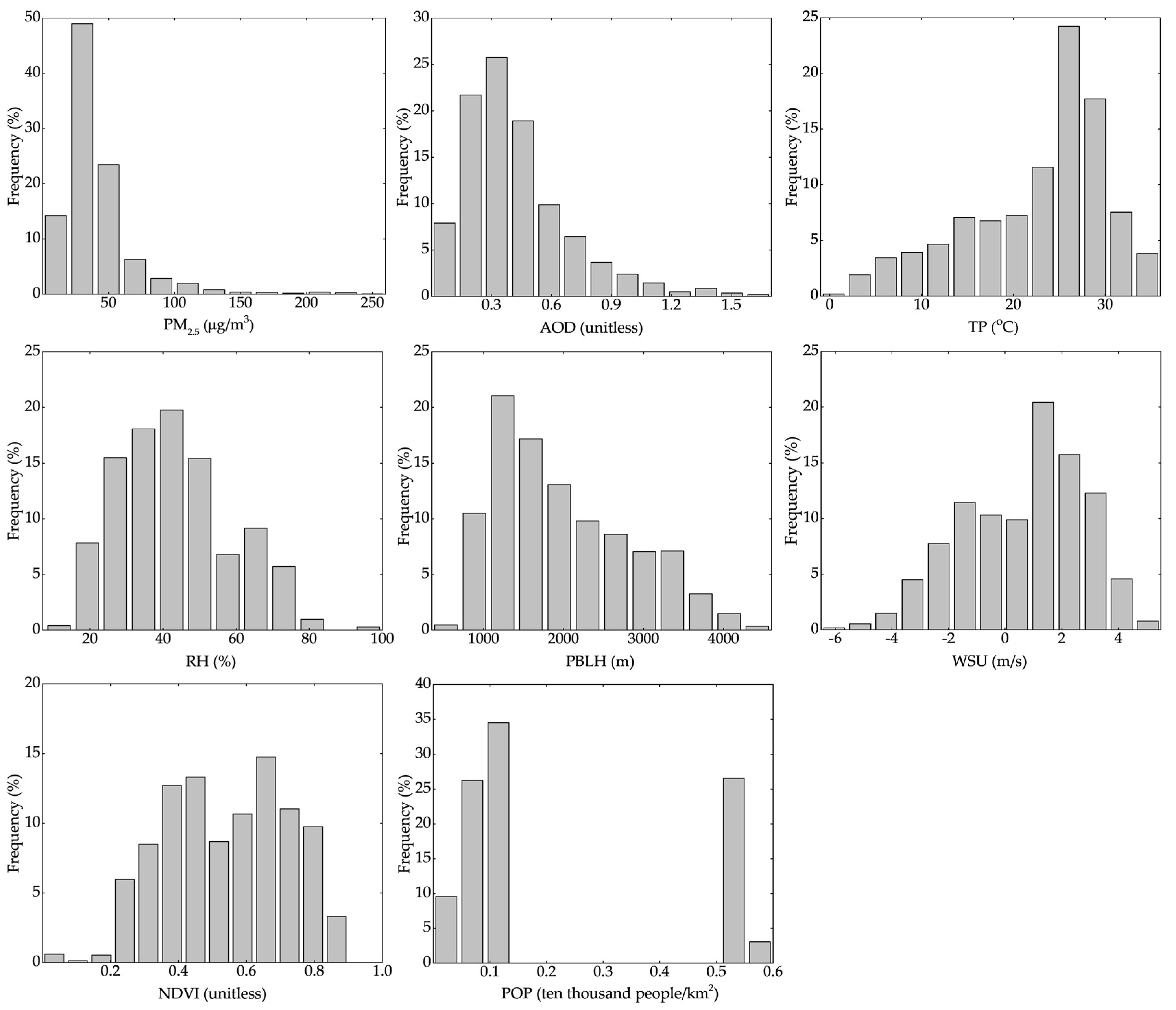
3.2. Data Overview and Characteristics

The VIIRS AOD datasets with QF = 3 were used for model development, together with collocated PM_2.5 and other data. The statistics of these data for each season and every city are presented in Tables S1 and S2 (Supplementary Materials), and the frequency distribution functions for the whole model fitting dataset are shown in the histograms of Figure 3. Seasons are defined here according to the actual seasonal division in the study area: spring (March, April, and May), summer (June, July, and August), autumn (September, October, and November), and winter (December, January, and February). Table S1 (Supplementary Materials) shows that the average PM_2.5 concentration and VIIRS AOD in the Guanzhong area for the whole year 2017 were 45.460 µg/m³ and 0.421, respectively. These results are about five times higher than the average concentrations of PM_2.5 and AOD in the eastern and southeastern United States [38,58], and the PM_2.5 concentration was much higher than the annual average concentration limit of 35 µg/m³ stipulated in the Environmental Air Quality Standard (http://kjs.mee.gov.cn/hjbhbz/bzwb/dqhjbh/dqhjzlbz/201203/W020120410330232398521.pdf, last access 1 November 2019), which was implemented by the Chinese Ministry of Environmental Protection in January 2016. This shows the severity of air quality problems in the Guanzhong area. Table S1 (Supplementary Materials) also shows that the annual wind speed in the study area was relatively low, ranging from −6.22 m/s to 5.353 m/s. The long-term static wind speed in the study area is also not conducive to the dispersion of pollutants. The data in Table S1 (Supplementary Materials) show that the PM_2.5 concentrations were highest in the winter, lowest in the summer, and moderate in the spring and autumn. The mean AOD values were similar in all seasons, but their median values changed. The study area is driest in the spring, and the wind speed does not vary much between seasons. Table S2 (Supplementary Materials) shows that PM_2.5 concentration was highest in Xi’an city, followed by Weinan city and Xianyang city, and lowest in Baoji city and Tongchuan city. The population density in Xi’an and Weinan is the largest, followed by Xianyang and Baoji, while Tongchuan has the lowest. Figure 3 shows that all variables except population density were approximately log-normally distributed with one single peak. We also calculated the variance inflation factor (VIF) between each of the independent variables to identify multicollinearity problems. When the threshold value of VIF is less than 2.5, it is considered that there is no multicollinearity phenomenon between variables [64]. The results show that the VIF values ranged from 0.000 to 1.333, and there was no multicollinearity problem in the model.

3.3. Predictor Factors Analysis

The fixed intercept b₀ and the slopes (i.e., coefficients b₁–b₇ in Equation (1)) of each predictor for the first-stage LME model are shown in

Table 2. Fixed effect of the liner mixed effects (LME) model. NDVI—normalized difference vegetation index; POP—population density; RH—relative humidity; PBLH—planetary boundary layer height; WSU—meridional component wind speed U; TP—temperature.

	Coefficient (bi)	p-Value
Intercept	58.848	0.000
AOD (unitless)	46.290	0.000
NDVI (unitless)	−10.282	0.003
POP (ten thousand people/km2)	1.478	0.192 a
RH (%)	−35.053	0.000
PBLH (m)	−0.009	0.087 b
WSU (m/s)	0.956	0.000
TP (°C)	0.057	0.000

^a The independent variable is not significant. ^b The independent variable is significant at the α = 0.1 level.

. For most variables (AOD, NDVI, RH, WSU, and TP), the results in Table 2 show that their effects on PM_2.5 were significant at the $\mathsf{\alpha }$ = 0.005 level, but POP appeared to have less influence. The spatial resolution of POP was the population density for each district or county, which was sparser than other variables. The sensitivity of PM_2.5 to changes in POP was low. As shown in Table 2, for AOD, POP, and TP the coefficients were positive, i.e., PM_2.5 concentrations increased with an increase in these parameters. NDVI, RH, and PBLH were negatively correlated with PM_2.5 concentrations.

It is worth noting that WSU was a positive coefficient in the equation. A positive value of WSU represents wind from west to east, and a negative value represents the wind from east to west. Thus, we could distinguish the effect of west-to-east and east-to-west wind for PM_2.5. The concentration of PM_2.5 in the Guanzhong area was positively correlated with the west-to-east wind. This is likely due to sandstorms in the desert area to the northwest of Guanzhong and transport of dust to the study area by westerly winds, leading to the increase in PM_2.5 concentrations [65]. However, in general, high wind speed results in the transport of pollution away from the area and, thus, smaller concentrations, while low wind speed leads to accumulation. Thus, the high east-to-west wind speed can increase horizontal and vertical mixing, thus diluting PM_2.5 concentration due to the dispersion of pollutants, which is negatively correlated with PM_2.5 concentrations [45].

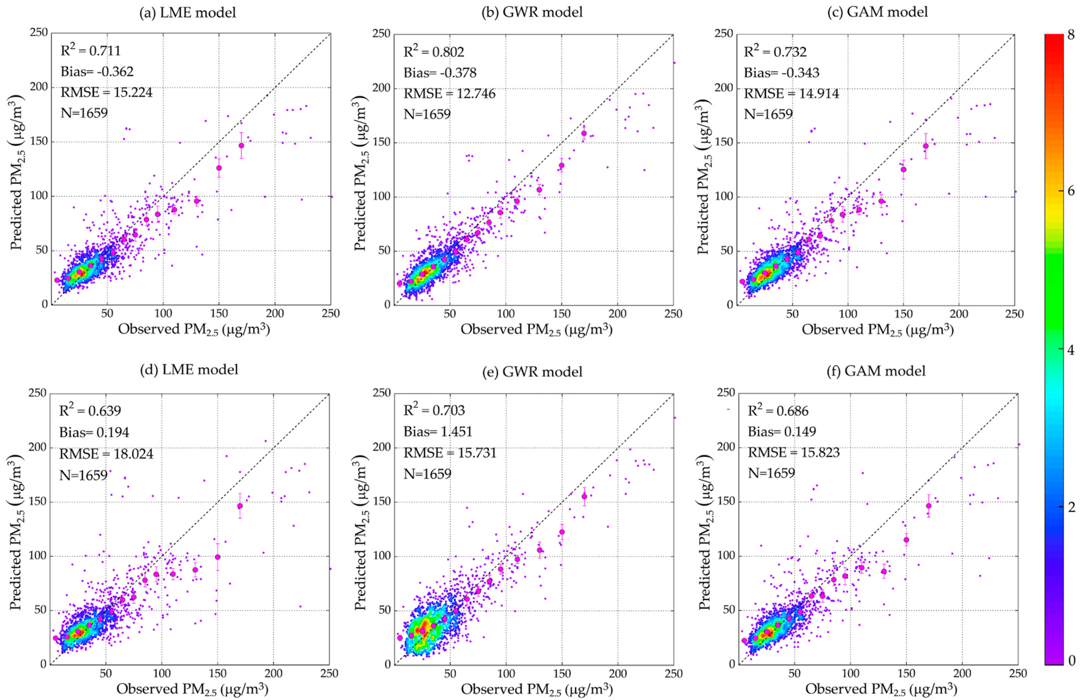
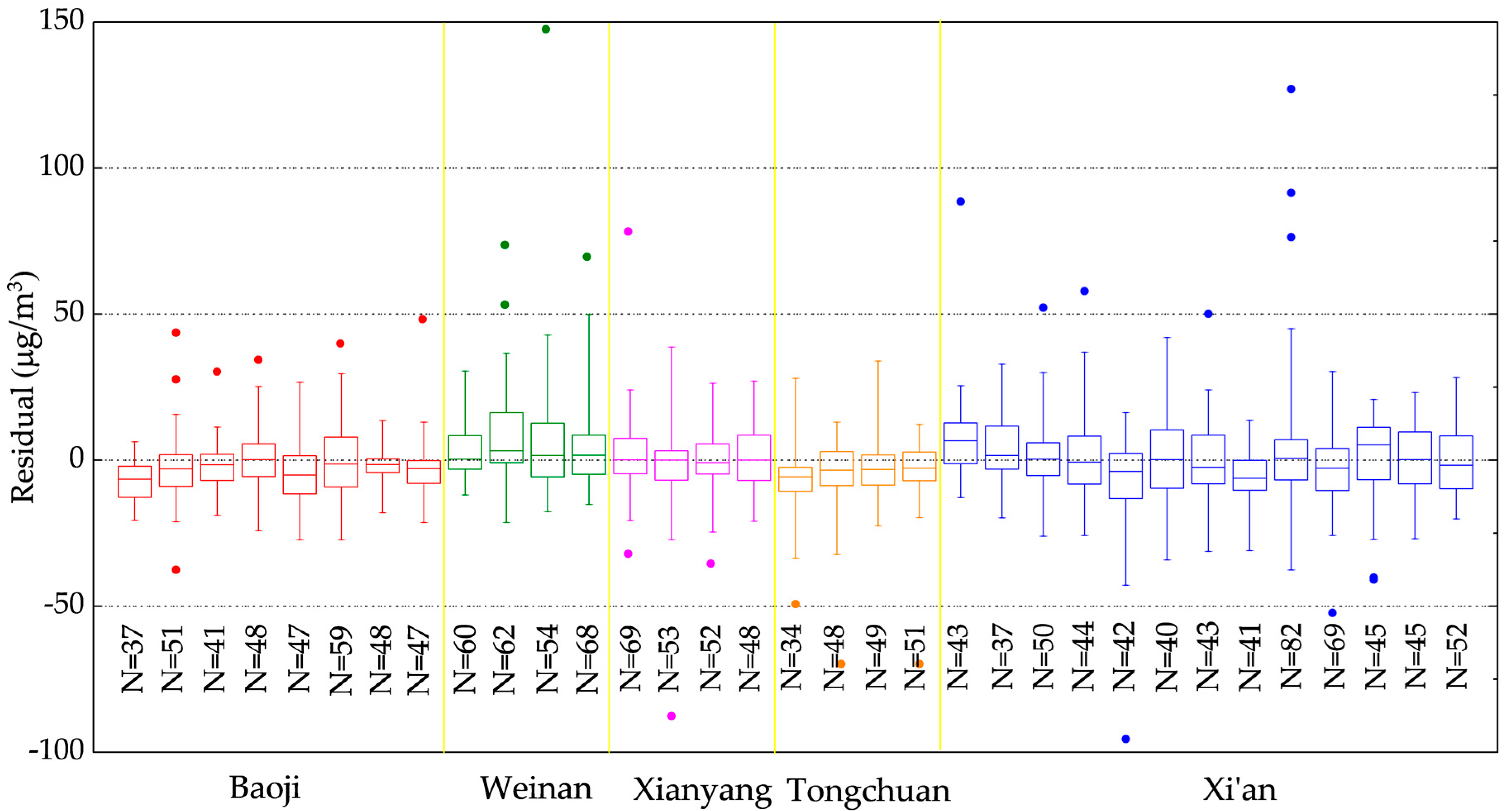
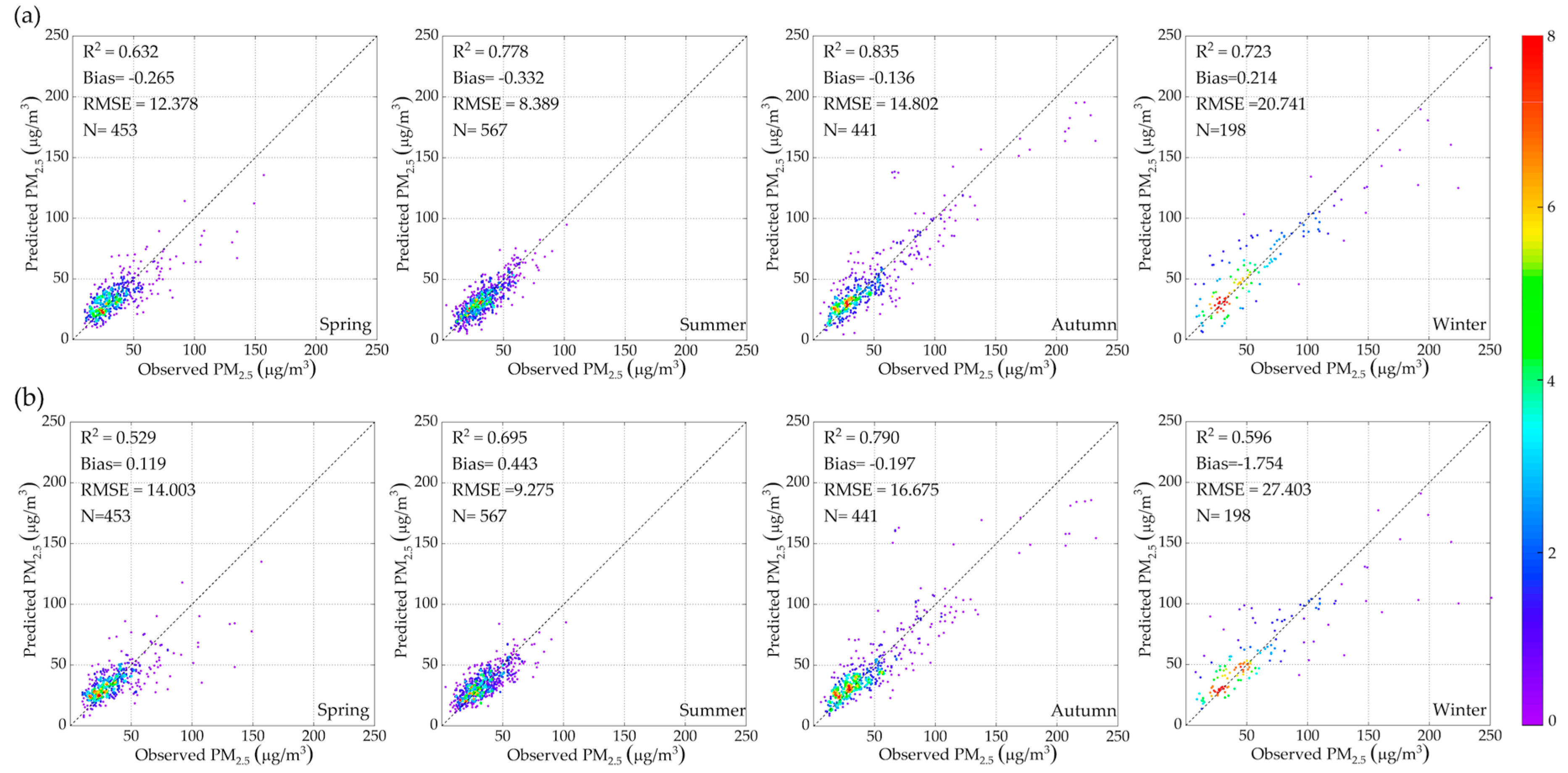
3.4. Model Validation

The LME model results were used in stage two to develop the GWR and GAM models as described in Section 2.3. To evaluate the model performance, the computed PM_2.5 concentrations were compared with the observations using model fitting (Figure 4a–c) and cross-validation (Figure 4d–f) methods as described in Section 2.4. A comparison of the results from the second-stage GWR model (Figure 4b) with those from the LME model (Figure 4a) shows that the inclusion of the temporal and spatial variability of the PM_2.5 concentration in the GWR model provided an improvement over the LME model (R² = 0.802 vs. 0.711; RMSE was also lower). The GAM model (Figure 4c) was also an improvement over the LME model but much less than that of GWR. For the low PM_2.5 concentrations (less than 30 µg/m³), all three models were overestimated. When PM_2.5 concentrations were larger than 40 µg/m³, all three models were underestimated, and as observed PM_2.5 concentrations increased, underestimation also increased. However, predicted values for the GWR model were much closer to the observations because it better captured the geographical variations of PM_2.5 after adding geolocation information into the model. Figure 4 shows that, for PM_2.5 concentrations larger than 140 µg/m³, underestimation occurred irrespective of whether model fitting or cross-validation was used. This may be because the model parameters were determined using mainly PM_2.5 concentrations smaller than 140 µg/m³, and high PM_2.5 values got less weight. Therefore, the results do not apply to such high values. Another possible reason is that the areas with high PM_2.5 concentrations are very local and not well captured by coarse spatial resolution [16].

The 10-fold cross-validation method was applied to the three models, LME, GAM, and GWR, to evaluate the predictive ability of each model for PM_2.5 over the Guanzhong area, using R², bias, and RMSE as metrics. The results in Figure 4 show that all models over-fitted for the training data; the R² values of all three models for CV (Figure 4e,f) were smaller than for model fitting (Figure 4a–c). Figure 4a,d show that the R² and RMSE values of cross-validation were 0.639 and 18.024 µg/m³, which were 7% lower than the R² and 2.800 µg/m³ higher (6%) than the RMSE for model fitting, Figure 4b,e show that, when the GWR model was used in the second stage, the model over-fitting became larger as the limited amount of data matched each day [56], where R² of cross-validation was 10% smaller, and RMSE was 2.985 µg/m³ higher (7%) for the annual average PM_2.5 as compared to the results of model fitting. Figure 4c,f show that the GAM model was slightly over-fitting; the R² of cross validation was 0.686, and it was only 5% lower than model fitting, while the RMSE was 15.823 µg/m³, which was 0.909 µg/m³ higher (2%) than the annual average PM_2.5 as compared with the results of model fitting. This also shows that the GAM model could improve the tendency of overestimation for low values and underestimation for high values to a degree. However, our results show that the GWR model with geographic location information improved significantly on the R² and RMSE of model fitting or cross-validation, and it improved the model prediction accuracy.

To show the plausibility of the second-stage geographic location models, we plotted the residuals for each site in every city from the first-stage LME model as box plots in Figure 5. The results show that the residuals were mostly in the range from −40 to 40 µg/m³. Overall, the PM_2.5 concentrations in Tongchuan city were underestimated, whereas, in Weinan city, they were overestimated; in other cities, both under- and overestimation occurred. This indicates that the PM_2.5 concentration over- or underestimation at the sites in the same city were similar, while differences occurred between cities, which supported the idea that the PM_2.5 concentration at each monitoring site is related to the spatial location.

3.5. Comparison of the GWR and GAM Model

Compared with the GWR model, the overall performance of the GAM model’s fitting ability was worse. The validation results in Figure 4e,f show that R² was slightly higher for the GWR model, while RMSE was similar for both models. The error bars in Figure 4b,c show, however, a larger scatter of the GAM model results for high PM_2.5 values, although, for lower PM_2.5, the GAM results were closer to the identity line. The GWR model used the AOD with the strongest correlation for PM_2.5 as an independent variable; thus, it could better improve the ability to capture the spatial variation of PM_2.5.

By analysis of the seasonal variation, we can also see the difference in the performance of each model in every season. This is illustrated in Figure 6, which shows scatter plots of the PM_2.5 values predicted by the GAM and GWR models versus ground-based observations for each season. The performances of the GWR and GAM models for each season were similar; they were best in the autumn (R² of 0.835 and 0.790) and the summer (R² of 0.778 and 0.695), while the winter (R² of 0.723 and 0.596) came third, and the spring (R² of 0.632 and 0.529) had the lowest correlations. This is probably because the vegetation is dense in autumn and summer, and the low wind speed results in the accumulation of aerosol particles in the Guanzhong area, enabling the model to best predict PM_2.5. In the winter, fewer AOD values can be retrieved due to the more frequent occurrence of clouds, and the chemical characteristics of particulate matter become more complex because of emissions due to indoor heating, coal burning, and festival fireworks, while vertical dispersion is also limited due to the lower inversion height. AOD is a columnar measurement of aerosol light extinction. The effect of aerosol characteristics (e.g., chemical composition and size distribution) are important in light extinction [66]. However, the effects of aerosol chemical characteristics and size distribution were not considered in this study. When the aerosol characteristics become more complex, the model cannot capture their effects on the PM_2.5/AOD relationship and, thus, also not on the model performance [66]. These factors may cause a distinct increase in PM_2.5 concentrations, resulting in a reduced ability of the model to correctly predict PM_2.5 [45,67]. PM_2.5 concentrations tend to be high in the winter and, therefore, the model performance is worse than in seasons with lower PM_2.5 concentrations. Dust storms have a significant impact on air quality in spring, i.e., the season with frequent desert dust storms and westerly and northwesterly winds which blow the dust into the Guanzhong area. Mineral dust concentrations are usually highest in late winter and early spring [68,69]. In these conditions, the predictive performance of PM_2.5 concentration was reduced.

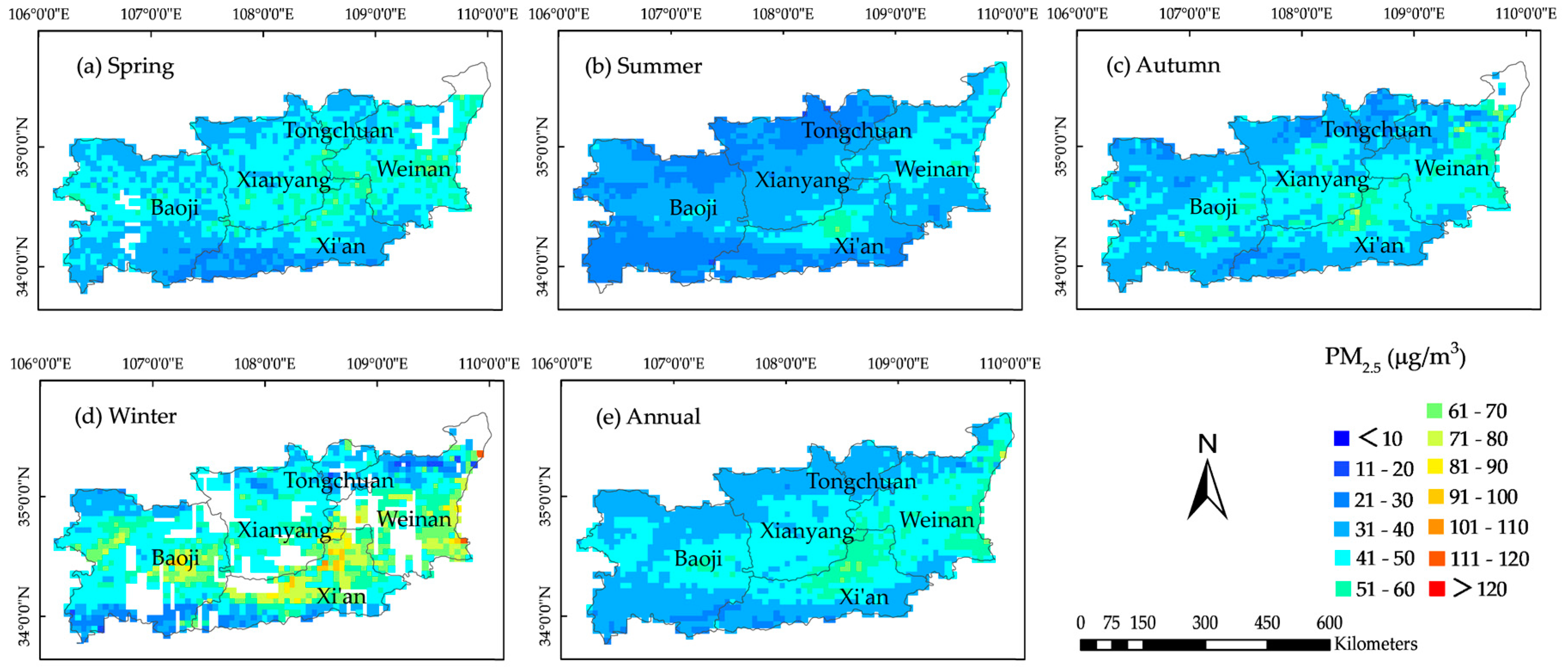
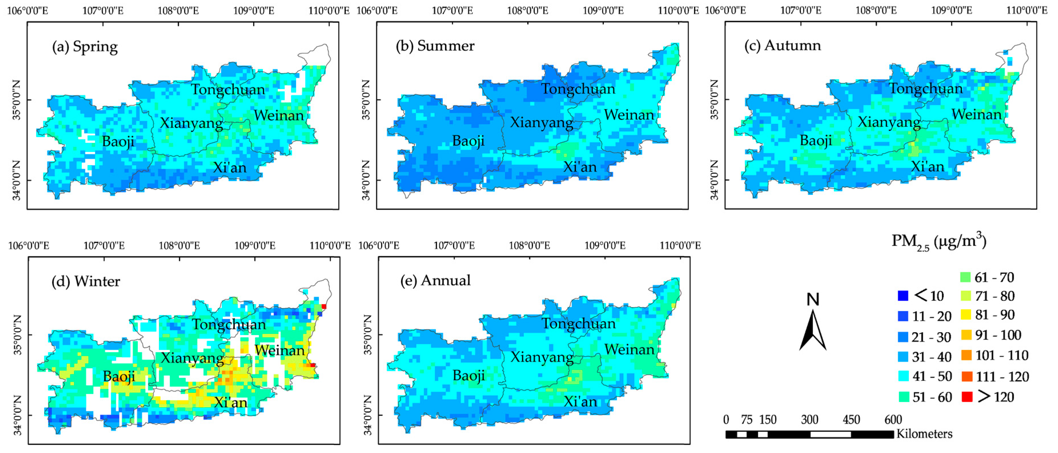
3.6. Temporal and Spatial Distributions of Predicted PM_2.5

The PM_2.5 concentration was calculated using the LME and GWR models for each pixel with 6 km × 6 km resolution around each of the PM_2.5 sites in the Guanzhong Basin, for every day of 2017. Using the results, the spatial variations of the average PM_2.5 concentrations over the study area were obtained for the whole year and for each season in 2017, with a spatial resolution of 6 km × 6 km. The results are presented in Figure 7 and Figure 8. The spatial distributions obtained from the LME and GWR models were very similar, but the concentrations predicted by the LME model were generally lower than those obtained from the GWR model, particularly in the winter when the PM_2.5 concentrations were highest. As described in Section 3.3 and Section 3.4, the LME model underestimated high PM_2.5 concentrations, but the addition of geographic location information using the GWR model improved the model performance. The GWR model shows the spatial distribution of PM_2.5 more accurately in conditions with high concentrations.

As shown in Figure 7 and Figure 8, PM_2.5 concentrations in Xi’an city were higher than in the other cities in the Guanzhong Basin. In the urban areas of Xi’an, the average annual PM_2.5 concentration was more than 70 µg/m³. Xi’an is the capital of Shaanxi Province and has the highest population density, traffic density, industrial production, combustion, etc., resulting in high PM_2.5 concentrations. Weinan and Xianyang are the second and third largest cities in terms of population density, with high urbanization and industrialization levels leading to high PM_2.5 concentrations. Baoji is located in the western part of the study area, and air quality is influenced by dust pollution from the northwest and industrial pollution advected from the east of the Guanzhong Basin under the action of atmospheric circulation. Tongchuan has the best air quality of the five cities in the study area. Figure 7 and Figure 8 show that the highest PM_2.5 concentrations in the Guanzhong Basin mainly occurred in the densely populated urban areas, with lower PM_2.5 concentrations in the suburbs or mountainous areas, especially in the southern part (i.e., Qinling Mountain) of Baoji and Xi’an with sparser population than in other areas. The PM_2.5 concentrations in the Guanzhong Basin have a clear seasonal variation. Winter was the most polluted season when the average PM_2.5 concentration in many areas was larger than 50 µg/m³. In the winter, temperature inversions occur frequently, and, in the shallow mixing layer, the dispersion of pollutants is limited, leading to accumulation and, thus, high concentrations near the ground. In addition, the smoke and dust released by centralized coal-fired power plants during the heating period contribute to the accumulation of fine particles, resulting in high PM_2.5 concentrations. In the summer, the PM_2.5 concentrations are the lowest of the year because of the most flourishing vegetation, the mainly sunny weather, the higher boundary layer, and the enhanced mixing in a developing atmospheric boundary layer. The PM_2.5 concentration levels in the spring and autumn were between those in the winter and summer. In spring, the climate in the Guanzhong area is dry, and local dust emission has a large influence on the urban pollution, in addition to desert dust transported into the area. The average PM_2.5 concentrations in the autumn were slightly lower than in the spring. Except in the northern part (Loess Plateau) and southern part (Qinling Mountains), the average annual PM_2.5 concentration in most areas of the Guanzhong Basin was higher than China’s ambient air quality standard (35 µg/m³) in 2017.

4. Discussion

In this study, we used AOD data, meteorological factors (PBLH, TP, and RH), NDVI, population density data, and a new variable, the wind speed vector of U component, to develop a model to estimate PM_2.5 concentrations. The effect of PBLH was significant at the α = 0. 1 level for PM_2.5, as also concluded from previous studies in Beijing, Tianjin, and Hebei [55] and across all of China [57]. Industrial activities and dense traffic occur in densely populated areas, and, together with other anthropogenic activities, the emissions of primary aerosol particles and aerosol precursor gases from these activities contribute to the increase in PM_2.5 concentration. Thus, the concentration of PM_2.5 in densely populated areas is usually high [70]. High temperature accelerates the secondary formation of particles from precursor gases such as SO₂, NO₂, and volatile organic compounds (VOCs), which may further grow due to condensation of vapors, which in turn leads to the increase in PM_2.5 concentration. NDVI is an indicator for the amount of vegetation which can effectively adsorb and remove particulate matter from the air due to the higher roughness, which results in higher dry deposition velocity [71]. The effect of relative humidity is twofold. Firstly, when RH increases, the particles grow due to condensation of water vapor, which implies dilution of the dissolved salts and, thus, lower specific mass, which, for particles in different RH environments but with the same diameter, results in differences in the dry mass when these particles are bought into a low-RH environment. Secondly, when the particles grow, the particle size distribution shifts to larger sizes. Because PM_2.5 monitors use an inlet designed to sample ambient (i.e., wet) particles with an aerodynamic diameter of 2.5 µm, a shift in the size distribution to larger particles results in missing a fraction of the particles that would be sampled at lower RH. Because the mass of this sample was determined after drying (in a low-RH environment), this results in another reduction in the particle mass. Hence, the mass of PM_2.5 decreases with increasing RH.

The effect of RH on AOD is the opposite. AOD is measured on ambient particles and, hence, the effect of particle growth usually results in an increase in the AOD. In fact, particles which, in dryer conditions, are too small to influence the scattering of solar radiation (smaller than about 0.05 μm, see Reference [72]) may grow and, thus, become optically active. Because the shape of the particle size distributions with high concentrations of particles is smaller than those for optically active particles (see, for instance, Reference [72]), this often implies an increase in the number of optically active particles and, thus, an increase in the particle scattering and also in the column-integrated extinction or AOD. The RH-induced variation of the extinction depends on the hygroscopic growth factor (i.e., chemical composition) [72].

With regard to the effect of the PBLH on PM_2.5, the planetary boundary layer (PBL) is the layer adjacent to the surface where vertical mixing takes place up to the inversion height (similar to the PBLH). When the air near the surface is heated by solar irradiation, it rises up to the PBLH where it encounters inversion (a temperature jump), while cooler air descends. This mechanism constitutes an effective mixing of the atmospheric constituents throughout the PBL and causes an increase in the PBLH until equilibrium is reached. As a result, aerosol particles are removed from the surface and effectively mixed throughout the PBL. Thus, surface concentrations such as those expressed by PM_2.5 become smaller when PBLH increases, but the total aerosol content in the PBL does not change and, thus, this process does not affect AOD. However, in a well-mixed PBL, the RH increases with height and, thus, particles may grow, which in turn causes the extinction coefficients to increase with height and, thus, also AOD.

In this paper, a model was presented to estimate temporal and spatial variations of surface PM_2.5 in the Guanzhong area with a higher spatial resolution of 6 km × 6 km than in previous studies that used the 10 km × 10 km MODIS AOD or the 17.6 km × 17.6 km MISR AOD. A new variable, WSU (wind speed vector into meridional component), was used to distinguish the effect of west-to-east and east-to-west winds in the study area. In addition, our research concentrated on the heavily polluted Guanzhong Basin area in China, where only few studies were carried out before. Generally, this study provides spatial details and information for PM_2.5 exposure, air pollution, and health impacts in the Guanzhong Basin, and provides guidance for preventing and controlling haze in cities.

Although VIIRS AOD had a satisfactory performance in estimating surface PM_2.5 concentrations, its shortcomings could not be ignored, and the research method of this paper had some limitations. The diurnal variability of PM_2.5 and AOD can be significant [73]. However, PM_2.5 concentrations and AOD values were only taken into account at one certain time of the day (VIIRS satellite overpass time) in this paper. The other times for all-day and daily cycles of PM_2.5 concentration could not be captured by satellite data [45]. This led to a certain bias in estimates of PM_2.5 concentration by using our model in the study area. The lack of satellite AOD retrieval in some conditions is a serious problem, such as in the winter for the study area, which is usually due to the presence of clouds or due to high reflectance of surfaces covered with snow or ice. These limitations are a generic feature of all AOD products [56]. The daily matchups of PM_2.5/AOD are primarily restricted by the lack of AOD observations, which was the reason that the LME model could not completely capture the random slopes and random intercepts for each day due to a decrease in precision. Moreover, the few daily matchups led to over-fitting of the model, which was addressed by the CV experiments in this paper. Therefore, the method to solve the problem of missing satellite AOD data will be one of the key points of our future research; we could use empirical gap-fitting methods to alleviate this problem [74]. There is the obvious seasonality of the PM_2.5 concentrations and the predictive ability of the model in the study area, which was closely related to the range of AOD values and PM_2.5 concentrations in different seasons. Different predictive models for different seasons could be developed to improve the prediction accuracy in each season and for every day. In addition, some auxiliary variables in past studies were not added to the model as independent variables because of data and resource limitations, such as wind vector data in four directions [29] and the traffic intensity and type (trucks and personal cars). The model’s stability and the accuracy of predicting spatio-temporal changes may be improved if we could add the above factors or add more suitable predictors to the model. Although a one-year study (2017) covers different meteorological conditions and seasons, the use of more years would show effects of year-to-year variations due to, for instance, changes in large-scale variations. In future research, more data could be collected for further analysis to evaluate the historical changes of PM_2.5 and the inter-annual changes of the relationship between PM_2.5 and AOD.

5. Conclusions

This study aimed to develop a two-stage model to estimate the surface PM_2.5 concentrations and the PM_2.5 spatio-temporal distribution in the heavily polluted Guanzhong Basin in China. We used VIIRS AOD data with a spatial resolution of 6 × 6 km² as the main prediction variable. Sun photometer data from the SONET ground monitoring station located in Xi’an were used to test the accuracy of VIIRS AOD products with different quality flags, and VIIRS AOD with QF = 3 was selected for use in this study. The main conclusions are as follows:

(1) The annual average PM_2.5 concentration in most areas of the Guanzhong Basin in 2017 was higher than China’s ambient air quality standard (35 µg/m³).

(2) The developed models do not apply the higher PM_2.5 concentration (i.e., more than 140 µg/m³) or some areas where high PM_2.5 concentrations are very local.

(3) The GWR and GAM models could improve the performance of the LME model; the GWR model alleviated the underestimation of the LME model, and its performance in capturing the temporal and spatial changes of PM_2.5 was better than that of the GAM model. The combined model prediction of PM_2.5 concentrations was more accurate in the summer and autumn than in the spring and winter.

(4) In the Guanzhong Basin area, PM_2.5 was well correlated with vegetation coverage and meteorological factors. PM_2.5 was positively correlated with temperature, population, and wind from west to east, and negatively correlated with vegetation cover, relative humidity, planetary boundary layer height, and wind from east to west. We recommend using VIIRS AOD QF = 3 products to estimate surface PM_2.5 concentrations.

(5) The topography and the population density had a strong influence on the spatial distribution pattern of PM_2.5 concentrations in the Guanzhong Basin; it was higher in Xi’an, Weinan, and Xianyang, but lower in Baoji and Tongchuan. Moreover, the PM_2.5 concentrations in the Guanzhong Basin varied with the seasons and were highest in the winter, moderate in the spring and autumn, and lowest in the summer.

References

1. Lee, H.; Chatfield, R.; Strawa, A. Enhancing the applicability of satellite remote sensing for PM2.5 estimation using MODIS deep blue AOD and land use regression in California, United States. Environ. Sci. Technol. 2016, 50, 6546–6555. [Google Scholar] [CrossRef] [PubMed]
2. Van Donkelaar, A.; Martin, R.V.; Brauer, M.; Boys, B.L. Use of satellite observations for long-term exposure assessment of global concentrations of fine particulate matter. Environ. Health Perspect. 2014, 123, 135–143. [Google Scholar] [CrossRef] [PubMed]
3. Van Donkelaar, A.; Martin, R.V.; Brauer, M.; Kahn, R.; Levy, R.; Verduzco, C.; Villeneuve, P.J. Global estimates of ambient fine particulate matter concentrations from satellite-based aerosol optical depth: Development and application. Environ. Health Perspect. 2010, 118, 847–855. [Google Scholar] [CrossRef] [PubMed]
4. Chatfield, R.B.; Sorek-Hamer, M.; Esswein, R.F.; Lyapustin, A. Satellite Mapping of PM2.5 Episodes in the Wintertime San Joaquin Valley: A “Static” Model Using Column Water Vapor. Atmos. Chem. Phys. Discuss. 2019, 262, 1–27. [Google Scholar]
5. Wang, H.; Li, J.; Peng, Y.; Zhang, M.; Che, H.; Zhang, X. The impacts of the meteorology features on PM2.5 levels during a severe haze episode in central-east China. Atmos. Environ. 2019, 197, 177–189. [Google Scholar] [CrossRef]
6. Van Donkelaar, A.; Martin, R.V.; Levy, R.C.; Silva, A.M.; Krzyzanowski, M.; Chubarova, N.E.; Semutnikova, E.; Cohen, A.J. Satellite-based estimates of ground-level fine particulate matter during extreme events: A case study of the Moscow fires in 2010. Atmos. Environ. 2011, 45, 6225–6232. [Google Scholar] [CrossRef]
7. Bouet, C.; Labiadh, M.T.; Rajot, J.L.; Bergametti, G.; Marticorena, B.; Henry des Tureaux, T.; Ltifi, M.; Sekrafi, S.; Féron, A.J.A. Impact of Desert Dust on Air Quality: What is the Meaningfulness of Daily PM Standards in Regions Close to the Sources? The Example of Southern Tunisia. Atmosphere 2019, 10, 452. [Google Scholar] [CrossRef]
8. Giannadaki, D.; Pozzer, A.; Lelieveld, J. Modeled global effects of airborne desert dust on air quality and premature mortality. Atmos. Chem. Phys. 2014, 14, 957–968. [Google Scholar] [CrossRef]
9. Sakhamuri, S.; Cummings, S. Increasing trans-Atlantic intrusion of Sahara dust: A cause of concern? Lancet Planet. Health 2019, 3, 242–243. [Google Scholar] [CrossRef]
10. Varga, G.; Cserháti, C.; Kovács, J.; Szeberényi, J.; Bradák, B. Unusual Saharan dust events in the Carpathian Basin (Central Europe) in 2013 and early 2014. Water 2014, 69, 309–313. [Google Scholar] [CrossRef]
11. Varga, G.; Roettig, C.B. Identification of Saharan dust particles in Pleistocene dune sand-paleosol sequences of Fuerteventura (Canary Islands). Hungarian Geogr. Bull. 2018, 67, 121–141. [Google Scholar] [CrossRef]
12. Rizwan, S.; Nongkynrih, B.; Gupta, S.K. Air pollution in Delhi: Its magnitude and effects on health. Indian J. Community Med. 2013, 38, 4. [Google Scholar] [PubMed]
13. Proestakis, E.; Amiridis, V.; Marinou, E.; Georgoulias, A.K.; Solomos, S.; Kazadzis, S.; Chimot, J.; Che, H.; Alexandri, G.; Binietoglou, I.; et al. Nine-year spatial and temporal evolution of desert dust aerosols over South and East Asia as revealed by CALIOP. Atmos. Chem. Phys. 2018, 18, 1337–1362. [Google Scholar] [CrossRef]
14. Boys, B.; Martin, R.; Van Donkelaar, A.; MacDonell, R.; Hsu, N.; Cooper, M.; Yantosca, R.; Lu, Z.; Streets, D.; Zhang, Q.; et al. Fifteen-year global time series of satellite-derived fine particulate matter. Environ. Sci. Technol. 2014, 48, 11109–11118. [Google Scholar] [CrossRef]
15. Van Donkelaar, A.; Martin, R.V.; Brauer, M.; Hsu, N.C.; Kahn, R.A.; Levy, R.C.; Lyapustin, A.; Sayer, A.M.; Winker, D.M. Global estimates of fine particulate matter using a combined geophysical-statistical method with information from satellites, models, and monitors. Environ. Sci. Technol. 2016, 50, 3762–3772. [Google Scholar] [CrossRef]
16. Ma, Z.; Hu, X.; Huang, L.; Bi, J.; Liu, Y. technology. Estimating ground-level PM2.5 in China using satellite remote sensing. Environ. Sci. Technol. 2014, 48, 7436–7444. [Google Scholar] [CrossRef]
17. Yao, F.; Wu, J.; Li, W.; Peng, J. A spatially structured adaptive two-stage model for retrieving ground-level PM2.5 concentrations from VIIRS AOD in China. ISPRS-J. Photogramm. Remote Sens. 2019, 151, 263–276. [Google Scholar] [CrossRef]
18. Atkinson, R.; Kang, S.; Anderson, H.; Mills, I.; Walton, H. Epidemiological time series studies of PM2.5 and daily mortality and hospital admissions: A systematic review and meta-analysis. Thorax 2014, 69, 660–665. [Google Scholar] [CrossRef]
19. Chung, Y.; Dominici, F.; Wang, Y.; Coull, B.A.; Bell, M.L. Associations between long-term exposure to chemical constituents of fine particulate matter (PM2.5) and mortality in Medicare enrollees in the eastern United States. Environ. Health Perspect. 2015, 123, 467–474. [Google Scholar] [CrossRef]
20. Peng, R.D.; Bell, M.L.; Geyh, A.S.; McDermott, A.; Zeger, S.L.; Samet, J.M.; Dominici, F. Emergency admissions for cardiovascular and respiratory diseases and the chemical composition of fine particle air pollution. Environ. Health Perspect. 2009, 117, 957–963. [Google Scholar] [CrossRef]
21. Ghosh, J.K.C.; Wilhelm, M.; Su, J.; Goldberg, D.; Cockburn, M.; Jerrett, M.; Ritz, B. Assessing the influence of traffic-related air pollution on risk of term low birth weight on the basis of land-use-based regression models and measures of air toxics. Am. J. Epidemiol. 2012, 175, 1262–1274. [Google Scholar] [CrossRef] [PubMed]
22. Pope, C.A., III; Hansen, J.C.; Kuprov, R.; Sanders, M.D.; Anderson, M.N.; Eatough, D.J.; Association, W.M. Vascular function and short-term exposure to fine particulate air pollution. J. Air Waste Manag. Assoc. 2011, 61, 858–863. [Google Scholar] [CrossRef] [PubMed]
23. Yang, G.; Wang, Y.; Zeng, Y.; Gao, G.F.; Liang, X.; Zhou, M.; Wan, X.; Yu, S.; Jiang, Y.; Naghavi, M.; et al. Rapid health transition in China, 1990–2010: Findings from the Global Burden of Disease Study 2010. Lancet 2013, 381, 1987–2015. [Google Scholar] [CrossRef]
24. Kokhanovsky, A.A.; Leeuw, G. Satellite Aerosol Remote Sensing over Land; Springer: Heidelberg, Germany, 2009. [Google Scholar]
25. Schaap, M.; Apituley, A.; Timmermans, R.; Koelemeijer, R.; Leeuw, G. Exploring the relation between aerosol optical depth and PM2.5 at Cabauw, the Netherlands. Atmos. Chem. Phys. 2009, 9, 909–925. [Google Scholar] [CrossRef]
26. Liu, Y.; Paciorek, C.J.; Koutrakis, P. Estimating regional spatial and temporal variability of PM2.5 concentrations using satellite data, meteorology, and land use information. Environ. Health Perspect. 2009, 117, 886–892. [Google Scholar] [CrossRef]
27. Xue, T.; Zheng, Y.; Geng, G.; Zheng, B.; Jiang, X.; Zhang, Q.; He, K. Fusing observational, satellite remote sensing and air quality model simulated data to estimate spatiotemporal variations of PM2.5 exposure in China. Remote Sens. 2017, 9, 221. [Google Scholar] [CrossRef]
28. He, Q.; Huang, B. Satellite-based mapping of daily high-resolution ground PM2.5 in China via space-time regression modeling. Remote Sens. Environ. 2018, 206, 72–83. [Google Scholar] [CrossRef]
29. Wu, J.; Yao, F.; Li, W.; Si, M. VIIRS-based remote sensing estimation of ground-level PM2.5 concentrations in Beijing–Tianjin–Hebei: A spatiotemporal statistical model. Remote Sens. Environ. 2016, 184, 316–328. [Google Scholar] [CrossRef]
30. Zheng, Y.; Zhang, Q.; Liu, Y.; Geng, G.; He, K. Estimating ground-level PM2.5 concentrations over three megalopolises in China using satellite-derived aerosol optical depth measurements. Atmos. Environ. 2016, 124, 232–242. [Google Scholar] [CrossRef]
31. Huang, W.; Cao, J.; Tao, Y.; Dai, L.; Lu, S.-E.; Hou, B.; Wang, Z.; Zhu, T. Seasonal variation of chemical species associated with short-term mortality effects of PM2.5 in Xi’an, a central city in China. Am. J. Epidemiol. 2012, 175, 556–566. [Google Scholar] [CrossRef]
32. Peng, Y.; Liu, X.; Dai, J.; Wang, Z.; Dong, Z.; Dong, Y.; Chen, C.; Li, X.; Zhao, N.; Fan, C. Aerosol size distribution and new particle formation events in the suburb of Xi’an, northwest China. Atmos. Environ. 2017, 153, 194–205. [Google Scholar] [CrossRef]
33. Chu, D.; Tsai, T.; Chen, J.; Chang, S.; Jeng, Y.; Chiang, W.; Lin, N. Interpreting aerosol lidar profiles to better estimate surface PM2.5 for columnar AOD measurements. Atmos. Environ. 2013, 79, 172–187. [Google Scholar] [CrossRef]
34. Zhang, Y.; Li, Z. Remote sensing of atmospheric fine particulate matter (PM2.5) mass concentration near the ground from satellite observation. Remote Sens. Environ. 2015, 160, 252–262. [Google Scholar] [CrossRef]
35. Wang, J.; Christopher, S. Intercomparison between satellite-derived aerosol optical thickness and PM2.5 mass: Implications for air quality studies. Geophys. Res. Lett. 2003, 30. [Google Scholar] [CrossRef]
36. Liu, Y.; Franklin, M.; Kahn, R.; Koutrakis, P. Using aerosol optical thickness to predict ground-level PM2.5 concentrations in the St. Louis area: A comparison between MISR and MODIS. Remote Sens. Environ. 2007, 107, 33–44. [Google Scholar] [CrossRef]
37. Lee, H.; Liu, Y.; Coull, B.; Schwartz, J.; Koutrakis, P. A novel calibration approach of MODIS AOD data to predict PM2.5 concentrations. Atmos. Chem. Phys. 2011, 11, 15. [Google Scholar] [CrossRef] [Green Version]
38. Hu, X.; Waller, L.A.; Al-Hamdan, M.Z.; Crosson, W.L.; Estes, M.G., Jr.; Estes, S.M.; Quattrochi, D.A.; Sarnat, J.A.; Liu, Y. Estimating ground-level PM2.5 concentrations in the southeastern US using geographically weighted regression. Environ. Res. 2013, 121, 1–10. [Google Scholar] [CrossRef]
39. Ma, Z.; Liu, Y.; Zhao, Q.; Liu, M.; Zhou, Y.; Bi, J. Satellite-derived high resolution PM2.5 concentrations in Yangtze River Delta Region of China using improved linear mixed effects model. Atmos. Environ. 2016, 133, 156–164. [Google Scholar] [CrossRef]
40. Liu, Y.; Cao, G.; Zhao, N.; Mulligan, K.; Ye, X. Improve ground-level PM2.5 concentration mapping using a random forests-based geostatistical approach. Environ. Pollut. 2018, 235, 272–282. [Google Scholar] [CrossRef]
41. Chen, G.; Li, S.; Knibbs, L.D.; Hamm, N.A.; Cao, W.; Li, T.; Guo, J.; Ren, H.; Abramson, M.J.; Guo, Y. A machine learning method to estimate PM2.5 concentrations across China with remote sensing, meteorological and land use information. Sci. Total Environ. 2018, 636, 52–60. [Google Scholar] [CrossRef]
42. Wang, W.; Zhao, S.; Jiao, L.; Taylor, M.; Zhang, B.; Xu, G.; Hou, H. Estimation of PM2.5 Concentrations in China using a spatial back propagation neural network. Sci. Rep. 2019, 9, 1–10. [Google Scholar] [CrossRef] [PubMed] [Green Version]
43. Jackson, J.M.; Liu, H.; Laszlo, I.; Kondragunta, S.; Remer, L.A.; Huang, J.; Huang, H. Suomi-NPP VIIRS aerosol algorithms and data products. J. Geophys. Res.-Atmos. 2013, 118, 12673–612689. [Google Scholar] [CrossRef]
44. Shen, Z.; Cao, J.; Liu, S.; Zhu, C.; Wang, X.; Zhang, T.; Xu, H.; Hu, T. Chemical composition of PM10 and PM2.5 collected at ground level and 100 meters during a strong winter-time pollution episode in Xi’an, China. J. Air Waste Manag. Assoc. 2011, 61, 1150–1159. [Google Scholar] [CrossRef] [PubMed] [Green Version]
45. You, W.; Zang, Z.; Pan, X.; Zhang, L.; Chen, D. Estimating PM2.5 in Xi’an, China using aerosol optical depth: A comparison between the MODIS and MISR retrieval models. Sci. Total Environ. 2015, 505, 1156–1165. [Google Scholar] [CrossRef]
46. Bei, N.; Xiao, B.; Meng, N.; Feng, T. Critical role of meteorological conditions in a persistent haze episode in the Guanzhong basin, China. Sci. Total Environ. 2016, 550, 273–284. [Google Scholar] [CrossRef]
47. Miller, S.D.; Hawkins, J.D.; Kent, J.; Turk, F.J.; Lee, T.F.; Kuciauskas, A.P.; Richardson, K.; Wade, R.; Hoffman, C. NexSat: Previewing NPOESS/VIIRS imagery capabilities. Bull. Am. Meteorol. Soc. 2006, 87, 433–446. [Google Scholar] [CrossRef]
48. Vermote, E.; Justice, C.; Csiszar, I. Early evaluation of the VIIRS calibration, cloud mask and surface reflectance Earth data records. Remote Sens. Environ. 2014, 148, 134–145. [Google Scholar] [CrossRef] [Green Version]
49. Xiao, Q.; Zhang, H.; Choi, M.; Li, S.; Kondragunta, S.; Kim, J.; Holben, B.; Levy, R.; Liu, Y. Evaluation of VIIRS, GOCI, and MODIS Collection 6 AOD retrievals against ground sunphotometer observations over East Asia. Atmos. Chem. Phys. 2016, 16, 1255–1269. [Google Scholar] [CrossRef] [Green Version]
50. Zheng, S.; Pozzer, A.; Cao, C.; Lelieveld, J. Long-term (2001–2012) concentrations of fine particulate matter (PM2.5) and the impact on human health in Beijing, China. Atmos. Chem. Phys. 2015, 15, 5715–5725. [Google Scholar] [CrossRef] [Green Version]
51. Li, Y.; Xue, Y.; Guang, J.; She, L.; Fan, C.; Chen, G. Ground-Level PM2.5 concentration estimation from satellite data in the Beijing area using a specific particle swarm extinction mass conversion algorithm. Remote Sens. 2018, 10, 1906. [Google Scholar] [CrossRef] [Green Version]
52. Li, Z.; Xu, H.; Li, K.; Li, D.; Xie, Y.; Li, L.; Zhang, Y.; Gu, X.; Zhao, W.; Tian, Q. Comprehensive study of optical, physical, chemical, and radiative properties of total columnar atmospheric aerosols over China: An overview of sun–sky radiometer observation network (SONET) measurements. Bull. Am. Meteorol. Soc. 2018, 99, 739–755. [Google Scholar] [CrossRef]
53. Li, Z.; Li, D.; Li, K.; Xu, H.; Chen, X.; Chen, C.; Xie, Y.; Li, L.; Li, L.; Li, W.J. Sun-sky radiometer observation network with the extension of multi-wavelength polarization measurements. Remote Sens. 2015, 19, 495–519. [Google Scholar]
54. Xie, Y.; Li, Z.; Li, D.; Xu, H.; Li, K. Aerosol optical and microphysical properties of four typical sites of SONET in China based on remote sensing measurements. Remote Sens. 2015, 7, 9928–9953. [Google Scholar] [CrossRef] [Green Version]
55. Yao, F.; Si, M.; Li, W.; Wu, J. A multidimensional comparison between MODIS and VIIRS AOD in estimating ground-level PM2.5 concentrations over a heavily polluted region in China. Sci. Total Environ. 2018, 618, 819–828. [Google Scholar] [CrossRef] [PubMed]
56. Hu, X.; Waller, L.A.; Lyapustin, A.; Wang, Y.; Al-Hamdan, M.Z.; Crosson, W.L.; Estes, M.G., Jr.; Estes, S.M.; Quattrochi, D.A.; Puttaswamy, S.J. Estimating ground-level PM2.5 concentrations in the Southeastern United States using MAIAC AOD retrievals and a two-stage model. Remote Sens. Environ. 2014, 140, 220–232. [Google Scholar] [CrossRef]
57. Ma, Z.; Hu, X.; Sayer, A.M.; Levy, R.; Zhang, Q.; Xue, Y.; Tong, S.; Bi, J.; Huang, L.; Liu, Y. Satellite-based spatiotemporal trends in PM2.5 concentrations: China, 2004–2013. Environ. Health Perspect. 2015, 124, 184–192. [Google Scholar] [CrossRef] [Green Version]
58. Liu, Y.; Sarnat, J.A.; Kilaru, V.; Jacob, D.J.; Koutrakis, P. Estimating ground-level PM2.5 in the eastern United States using satellite remote sensing. Environ. Sci. Technol. 2005, 39, 3269–3278. [Google Scholar] [CrossRef] [Green Version]
59. Tan, W. The Basic Theoretics and Application Research on Geographically Weighted Regression. Ph.D. Thesis, Tongji University, Shanghai, China, 2007. [Google Scholar]
60. Ma, Z. Study on Spatiotemporal Distributions of PM2.5 in China Using Satellite Remote Sensing. Ph.D. Thesis, Nanjing University, Nanjing, China, 2015. [Google Scholar]
61. Wood, S.N. Generalized Additive Models: An Introduction with R; Chapman and Hall/CRC: London, UK, 2017. [Google Scholar]
62. Rodriguez, J.D.; Perez, A.; Lozano, J.A. Sensitivity analysis of k-fold cross validation in prediction error estimation. IEEE Trans. Pattern Anal. Mach. Intell. 2009, 32, 569–575. [Google Scholar] [CrossRef]
63. Wang, W.; Pan, Z.; Mao, F.; Gong, W.; Shen, L. Evaluation of VIIRS Land Aerosol Model Selection with AERONET Measurements. Int. J. Environ. Res. Public Health 2017, 14, 1016. [Google Scholar] [CrossRef] [Green Version]
64. Jongh, P.; Jongh, E.; Pienaar, M.; Gordon-Grant, H.; Oberholzer, M.; Santana, L. The impact of pre-selected variance in ation factor thresholds on the stability and predictive power of logistic regression models in credit scoring. ORiON 2015, 31, 17–37. [Google Scholar] [CrossRef] [Green Version]
65. Tsai, Y.I.; Chen, C. Characterization of Asian dust storm and non-Asian dust storm PM2.5 aerosol in southern Taiwan. Atmos. Environ. 2006, 40, 4734–4750. [Google Scholar] [CrossRef]
66. Lin, C.; Li, Y.; Yuan, Z.; Lau, A.; Li, C.; Fung, J. Using satellite remote sensing data to estimate the high-resolution distribution of ground-level PM2.5. Remote Sens. Environ. 2015, 156, 117–128. [Google Scholar] [CrossRef]
67. Wu, C.; Wang, G.; Wang, J.; Li, J.; Ren, Y.; Zhang, L.; Cao, C.; Li, J.; Ge, S.; Xie, Y. Chemical characteristics of haze particles in Xi’an during Chinese Spring Festival: Impact of fireworks burning. J. Environ. Sci. 2018, 71, 179–187. [Google Scholar] [CrossRef] [PubMed]
68. Zhang, X.Y.; Cao, J.; Li, L.; Arimoto, R.; Cheng, Y.; Huebert, B.; Wang, D. Characterization of atmospheric aerosol over XiAn in the south margin of the Loess Plateau, China. Atmos. Environ. 2002, 36, 4189–4199. [Google Scholar] [CrossRef]
69. Cao, J.; Lee, S.; Zhang, X.; Chow, J.C.; An, Z.; Ho, K.; Watson, J.G.; Fung, K.; Wang, Y.; Shen, Z. Characterization of airborne carbonate over a site near Asian dust source regions during spring 2002 and its climatic and environmental significance. J. Geophys. Res.-Atmos. 2005, 110, D3. [Google Scholar] [CrossRef] [Green Version]
70. Qi, M.; Jiang, L.; Liu, Y.; Xiong, Q.; Sun, C.; Li, X.; Zhao, W.; Yang, X. Analysis of the characteristics and sources of carbonaceous aerosols in PM2.5 in the Beijing, Tianjin, and Langfang region, China. Int. J. Environ. Res. Public Health 2018, 15, 1483. [Google Scholar] [CrossRef] [Green Version]
71. McDonald, A.; Bealey, W.; Fowler, D.; Dragosits, U.; Skiba, U.; Smith, R.; Donovan, R.; Brett, H.; Hewitt, C.; Nemitz, E. Quantifying the effect of urban tree planting on concentrations and depositions of PM10 in two UK conurbations. Atmos. Environ. 2007, 41, 8455–8467. [Google Scholar] [CrossRef]
72. Sundström, A.; Nikandrova, A.; Atlaskina, K.; Nieminen, T.; Vakkari, V.; Laakso, L.; Beukes, J.; Arola, A.; van Zyl, P.; Josipovic, M.; et al. Characterization of satellite-based proxies for estimating nucleation mode particles over South Africa. Atmos. Chem. Phys. 2015, 15, 4983–4996. [Google Scholar] [CrossRef] [Green Version]
73. Song, J.; Xia, X.; Che, H.; Wang, J.; Zhang, X.; Li, X. Daytime variation of aerosol optical depth in North China and its impact on aerosol direct radiative effects. Atmos. Environ. 2018, 182, 31–40. [Google Scholar] [CrossRef]
74. Kloog, I.; Koutrakis, P.; Coull, B.A.; Lee, H.J.; Schwartz, J. Assessing temporally and spatially resolved PM2.5 exposures for epidemiological studies using satellite aerosol optical depth measurements. Atmos. Environ. 2011, 45, 6267–6275. [Google Scholar] [CrossRef]
Figure 1. Elevation map of the study area, i.e., the Guanzhong Basin in the Shaanxi Province, China. Elevation is indicated by the color, see legend. Also shown are five cities, major highways, major railways, the air quality, and sun–sky radiometer observation network (SONET) stations in the study area.
Remotesensing 11 02679 g001
Figure 2. Scatter plots of Visible Infrared Imaging Radiometer Suite (VIIRS) aerosol optical depth (AOD) at 550 nm vs. SONET AOD at 500 nm for quality flag (QF) = 2 or 3 (a) and for QF = 3 (b) at the Xi’an site. The black dashed line is the identity line. Statistics in the upper left corner indicate coefficient of determination (R2), bias, root-mean-squared prediction error (RMSE), and number of data points (N).
Remotesensing 11 02679 g002
Figure 3. Histograms of dependent and independent variables in the model fitting dataset.
Remotesensing 11 02679 g003
Figure 4. Results of predicted PM2.5 (dry mass concentration of particles with an in situ aerodynamic diameter smaller than 2.5 µm) vs. observed PM2.5 for model fitting (ac) and cross-validation (df). For details on the 10-fold cross validation method, see Section 2.4. The filled circles are the averaged predicted PM2.5 binned in 10 µg/m3 observed PM2.5 intervals (20 µg/m3 for observed PM2.5 >100 µg/m3), and the vertical lines on each circle represent error bars (the 1σ SD of the fits). Statistics in the upper left corner indicate coefficient of determination (R2), bias (µg/m3), root-mean-squared prediction error (RMSE, µg/m3), and number of data points (N). The color bar on the right indicates the number of data points.
Remotesensing 11 02679 g004
Figure 5. The PM2.5 residuals (µg/m3) at each monitoring site in the five cities: Baoji, Weinan, Xianyang, Tongchuan, and Xi’an. The solid line in every box is the median for each site. The top of the box is the upper quartile, while the bottom of the box is the lower quartile. The lines on the box are the maximum and minimum values, respectively. The colored circles are outliers of residuals for every site. N is the number of data points for each station.
Remotesensing 11 02679 g005
Figure 6. Seasonal comparisons of PM2.5 concentrations predicted by the geographically weighted regression (GWR) (a) and generalized additive model (GAM) (b) vs. ground-based observations.
Remotesensing 11 02679 g006
Figure 7. PM2.5 concentrations in the Guanzhong Basin as predicted by the LME model, averaged over the year 2017 and for each of the seasons in 2017.
Remotesensing 11 02679 g007
Figure 8. Same as Figure 7, but predicted by the GWR model.
Remotesensing 11 02679 g008