Introduction of Variable Correlation for the Improved Retrieval of Crop Traits Using Canopy Reflectance Model Inversion

Abstract

Look-up table (LUT)-based canopy reflectance models are considered robust methods to estimate vegetation attributes from remotely sensed data. However, the LUT inversion approach is sensitive to measurements and model uncertainties, which raise the ill-posed inverse problem. Therefore, regularization options are needed to mitigate this problem and reduce the uncertainties of estimates. In this study, we introduce a new method to regularize the LUT inversion approach to improve the accuracy of biophysical parameters (leaf area index (LAI) and fractional vegetation cover (fCover)). This was achieved by incorporating known variable correlations that existed at the test site into the LUT approach to correlate the model variables of the Soil–Leaf–Canopy (SLC) model using the Cholesky decomposition algorithm. The retrievals of 27 potato plots obtained from the regularized LUT (LUTreg) were compared with the standard LUT (LUTstd), which did not consider variable correlations. Different solutions from both types of LUTs (LUTreg and LUTstd) were utilized to improve the quality of the model outputs. Results indicate that the present method improved the accuracy of LAI estimation, with the coefficient of determination R² = 0.74 and normalized root-mean-square error NRMSE = 24.45% in LUTreg, compared with R² = 0.71 and NRMSE = 25.57% in LUTstd. In addition, the variability of LAI decreased in LUTreg (5.10) compared with that in LUTstd (12.10). Hence, our results give new insight into the impact of adding the correlation between variables to the LUT inversion approach to improve the accuracy of estimations. In this study, only two correlated variables (LAI and fCover) were examined; in subsequent studies, the full correlation matrix based on the Cholesky algorithm should be explored.

1. Introduction

The quantitative estimation of vegetation characteristics from hyperspectral remote sensing is required for various applications in agriculture, ecology, plant physiology and meteorology [1,2]. In the agricultural context, among many vegetation characteristics, leaf area index (LAI), chlorophyll content and fractional vegetation cover (fCover) are of prime importance for crop production, crop phenotyping and precision farming [1,3,4]. LAI, a key attribute of vegetation structure, is related to gas exchange processes and the final production of crops [5,6], while fCover is used to monitor vegetation growth [7]. Chlorophyll content is an essential variable for photosynthesis and plant functioning and can serve as an indicator of plant nitrogen content [8]. Chlorophyll content can be defined either at the leaf level (leaf chlorophyll content, LCC) or at the canopy level (canopy chlorophyll content, CCC, that is, the product of LAI and LCC) [9].

To derive vegetation attributes from hyperspectral remote sensing data, empirical (statistical) [4,10,11], physically based (using radiative transfer models (RTMs)) [12,13,14,15] or hybrid approaches can be used [16,17]. In the physically based approach, the interaction between solar radiation and vegetation is represented by RTMs based on physical laws [16,18]. RTMs can be utilized in either the forward or inverse (backward) mode. Using RTMs in the forward mode is an effective way to understand the model’s behavior and the impact of parameterizing the model variables on the simulated canopy reflectance [19]. The inverse mode is applied to retrieve the biophysical and biochemical variables associated with a certain canopy reflectance spectrum [20]. RTMs are required to be well suited for the crop type under study. For homogeneous and continuous canopies, a large number of studies have successfully used PROSAIL (a combination of the PROSPECT leaf model and the SAIL canopy model) [21]. For row crops (heterogeneous and discontinuous crop) such as potato, the SLC (Soil–Leaf–Canopy model [22], which is an extended version of the PROSAIL model, seems to be more suitable because it can accommodate for both (homogeneous and heterogeneous) canopy structures. Moreover, compared with more complex 3D models, the SLC model is more simple and requires less information on canopy structure [23]; it can directly retrieve the fCover variable from two basic input variables—LAI and vertical crown cover (Cv) [24].

Researchers have suggested many different inversion strategies, including look-up tables [15,20]; numerical optimization [25,26]; and machine learning-based inversion methods, such as artificial neural networks [13,27,28,29], genetic algorithms [30], support vector machines [31] and Bayesian system [24,32,33]. Among inversion strategies, the look-up table (LUT) constitutes a commonly used and robust approach for inverting an RTM [34]. The aim of the present study is to improve this method for more accurate retrievals of plant properties.

One general limitation of RTM inversion is the “ill-posed” problem. The root of this problem is that several combinations of variables result in similar spectra that are closest to the actual remote sensing observations [20,35]. Moreover, the measurement and model uncertainties may also induce high inaccuracy in the simulated reflectance spectra [26,36,37]. Several regularization schemes have been proposed to mitigate this problem and obtain more stable and reliable solutions (estimated parameters) [20]: using a priori information [38]; increasing data dimensionality (i.e., multi-angular, multi-temporal) [39]; the selection of proper cost functions [34,40,41]; wavelength selection [12,13,34,42,43]; the use of multiple solutions [12]; and the addition of Gaussian noise [34,44,45,46].

In this study, a new regularization method for the LUT inversion approach is proposed in which the variance–covariance structure among variables is considered in the simulation. Generally, previous studies have explicitly treated the input parameters of RTMs independently to generate a range of simulated canopy reflectances [47]. However, in reality, certain variables are intercorrelated (e.g., LAI and fCover). Considering the correlation between model variables, which is an additional source of a priori information, may prevent a mismatch during the sampling of the LUT input space and thus result in realistic variable combinations. This, in turn, may prevent the generation of meaningless canopy spectra and thereby improve the retrieval process [47].

There are different methods that can be applied to transform independent random variables to correlated ones. However, compared with other methods, the Cholesky decomposition algorithm is simpler, computationally faster, and insensitive to the sampling error in a small sample size, and it works for nonlinear data distributions [48,49,50,51]. As shown in previous studies, the Cholesky algorithm with the nonparametric regression approach can be employed to derive biophysical and biochemical parameters [52,53]. Nevertheless, this algorithm has not yet been applied directly to physical models (RTMs) to retrieve the corresponding parameters [34].

The present study intends to address the following research question: To what extent does integrating the correlation structure of selected variables into the LUT inversion approach using the SLC model improve the retrieval of LAI and fCover? We hypothesized that adding a known relation between variables to the LUT (denoted as regularized LUT (LUTreg)) would increase the accuracy of LAI and fCover retrievals compared with the standard LUT (LUTstd). Besides addressing the relation between variables, an existing regularization technique (multiple solutions) was examined as an additional means of stabilizing the LUT retrieval approach. Retrievals from both types of LUTs (LUTreg and LUTstd) were validated by in situ measurements and systematically compared to highlight the added value of using variable relation in the generation of LUT.

2. Materials and Methods

2.1. Study Area and Experimental Design

The study area is located in the southwest of Luxembourg 49°36′47.1″N, 5°55′6.7″E (Figure 1A). It is characterized by a temperate climate with an annual average precipitation of about 700 mm and different loam soil textures, which are mainly sandy loams. The experiment was established in 2016 during the spring season. In this experiment, an agricultural parcel was planted with a potato crop (Victoria cultivar). Plots (5 × 3 m) with three nitrogen fertilization levels were established (80, 180, and 280 kg/ha nitrogen), representing under-, standard, and over-fertilization, respectively (Figure 1B). For each fertilization level, nine replicates were realized, resulting in a total sample of 27 plots. Measurements of canopy reflectance and vegetation parameters were taken on 20 July 2016, under cloud-free conditions with a blue sky. The plants’ growth stage was tuber bulking, flowering or both. Measurements were taken in the middle area of each plot, along with the positions shown in Figure 1C, to avoid border effects. The three nitrogen levels created different growth conditions, which resulted in a variation in biophysical and biochemical variables.

2.2. Spectral Measurements and Preprocessing

Canopy reflectance was measured by an ASD FieldSpec-3 spectroradiometer (Analytical Spectral Devices, Boulder, CO, USA) over 27 plots in a spectral range of 350–2500 nm. Spectral measurements were taken from a distance of about 80 cm above the canopy. Given the sensor field of view of 25°, the effective area of the footprint was 0.88 cm². An average of eight measurements at distributed positions (Figure 1C) was used to represent the reflectance of a plot. The measurements were obtained at the nadir position under direct solar illumination between 11:30 a.m. and 2:00 p.m. in order to minimize solar angle effects. The spectral bands in the water absorption region (1350–1460 nm, 1790–1960 nm, and above 2400 nm) and in the ozone region (bands below 400 nm) (21 bands in total) were excluded from further analysis. This is because these are noisy bands where the atmosphere strongly absorbs energy, leading to poor signal strength and errors in the analysis. In addition, a shift correction was applied to correct for effects caused by the three detectors [54]. For further analysis, the spectra were resampled to a 10 nm resolution, resulting in 180 wavebands.

2.3. Biophysical and Biochemical Measurements

LAI was measured nondestructively with a Licor LAI-2000 device. Measurements were taken in the morning under clear sky conditions and low sun angles by an operator who stood with his back toward the sun, and the measured plot was shielded from direct sun illumination using a large umbrella. Figure 1C shows the exact locations of below-canopy readings (red crosses). Readings above the canopy were taken before and after the below-canopy readings. The set of above- and below-canopy readings were averaged for each plot. fCover was visually estimated by a trained person in steps of 5% by looking from above in vertical direction on the canopy at the plot level [13]. LAI and fCover measurements were used for validation to evaluate the accuracy of estimated LAI and fCover, as well as for estimating the values of the leaf inclination distribution function (Section 2.5). The SPAD-502 Konica Minolta device was used to estimate leaf chlorophyll content. It is a nondestructive method of measuring the leaf transmittance using two wavelengths in the red spectral range (650 nm) and the near-infrared spectral range (940 nm). Six leaves per plot were selected randomly, and the average value of five readings per leaf from different positions of top leaflet was determined. The relative values of the SPAD readings were converted into leaf chlorophyll content per leaf surface area, expressed in $\mathsf{\mu }$g cm${}^{-2}$, using an empirical model for potato [55].

In Equation (1), LCC is the absolute amount of chlorophyll in $\mathsf{\mu }$mol m${}^{-2}$, and SPAD is a dimensionless value. With the molecular mass of chlorophyll a and chlorophyll b, units were converted from $\mathsf{\mu }$mol m${}^{-2}$ to $\mathsf{\mu }$g cm${}^{-2}$.

$$LCC\left(\mu gc{m}^{-2}\right)=0.0913\ast e^{0.0415\ast SPAD}$$

(1)

The total canopy chlorophyll content (CCC) for each plot was calculated by

$$CCC\left(g{m}^{-2}\right)=LCC\ast LAI$$

(2)

2.4. Radiative Transfer Model

In this study, a modified version of the Soil–Leaf–Canopy radiative transfer model (SLC) was employed [24]. SLC is an integrated model that combines the SAIL and geometric models to simulate reflectance from discontinuous canopies. Three submodels—the modified Hapke’s soil module [56], the modernized canopy module 4SAIL2 [22], and the PROSPECT-4 leaf module [57]—are combined in SLC. It simulates canopy bidirectional reflectance over a spectral range of 400–2500 nm at a 10 nm spectral resolution for arbitrary sun–target–sensor geometries. An amended version of the SAIL model is 4SAIL2, which includes the crown clumping (in the horizontal direction) and leaf color gradients (in the vertical direction) of a canopy. It simulates the bidirectional reflectance factor of a turbid medium plant by solving the scattering and absorption of four upward/downward radiative fluxes [22]. The input variables include LAI, the leaf inclination distribution function (LIDF), hotspot (hot), the layer dissociation factor (D), fraction brown leaf (fB), the tree shape factor (zeta), and vertical crown coverage (Cv). The last two parameters (zeta and Cv) describe the crown clumping effect, while D and fB characterize the distribution of brown and green leaves between the upper and lower layers of the canopy. The fraction of ground data covered by crowns in the nadir direction is calculated by directly determining the effective fractional vegetation cover or crown fraction (fCover) by two input parameters, LAI and Cv, as follows [24]:

$$fCover=Cv\ast (1-e^{-k\ast LAI}),$$

(3)

where Cv is the vertical crown cover, and $e^{-k\ast LAI}$ is the gap fraction following the Lambert–Beer law, and k is the extinction coefficient in the vertical direction and depends on the leaf inclination distribution function (LIDF) and the viewing angle ($\Theta$).

As input parameters, 4SAIL2 requires the directional-hemispherical reflectance and transmittance of a single leaf for both green and brown pigments to discriminate between photosynthetic and non-photosynthetic light absorption, which are supplied by the PROSPECT-4 model. This model is an updated version of PROSPECT, which does not have biochemical data pertaining to brown material [58]. The input variables of the PROSPECT-4 model are the leaf structure parameter (N) and leaf biochemical constituents, including leaf chlorophyll content (LCC), leaf dry matter content (Cm), leaf water content (Cw), and leaf senescent matter content (Cs).

2.5. Model Parameterization

The look-up table (LUT) approach was used in the forward mode to generate a set of simulated canopy reflectances from the table of input variables and to adapt the model for the potato crop. Some input variables (hotspot, dry matter, water content, senescent material, fraction brown leaf, the dissociation factor, and the zeta parameter) were effectively fixed using the values reported in

Table 1. Overview of the input variables in both types of look-up tables (LUTs) used for generating canopy spectra and for retrieving the target variables.

Parameter	Unit	Range		Fixed Value		Source of Information
		Min	Max
Leaf parameter (PROSPECT-4)
Internal leaf structure, N	Unitless	1	2.5			Kooistra and Clevers [10], Botha et al. [59]
Leaf chlorophyll content, LCC	($\mathsf{\mu }$g cm${}^{-2}$)	50	90			Field measurement
Water content, Cw	(cm)			0.0317		Clevers and Kooistra [8]
Dry matter content, Cm	(g cm${}^{-2}$)			0.005		Botha et al. [59]
Senescent material, Cs	Unitless			0		From field experience
Canopy parameter (4SAIL2)
Leaf area index, LAI	(m${}^2$ m${}^{-2}$)	0.4	5			Field measurement
Leaf inclination distribution function (LIDFa/b)	Unitless			0.66	−0.04	Estimated from comparison with field spectra
Hotspot coefficient, hot	(m m${}^{-1}$)			0.05		Casa and Jones [60]
Vertical crown cover, Cv	Unitless	0.1	1			From field experience
Tree shape factor, zeta	Unitless			2		From field experience
Layer dissociation factor, D	Unitless			1		From field experience
Solar zenith angle, tts	degree			38		Field measurement
Viewing zenith angle, tto	degree			0		-
Relative azimuth angle, psi	degree			0		-
Soil parameters (Hapke’s soil)
Hapke_b	Unitless			0.84		Verhoef and Bach [22], Mousivand et al. [24]
Hapke_c	Unitless			0.68		-
Hapke_h	Unitless			0.23		-
Hapke_B0	Unitless			0.3		-
Soil moisture, SM	Unitless			15		From field experience

, while the other variables were kept free because of the high sensitivity of canopy spectra. From the prior information from the field, previous studies, and user experience, the bounds and ranges of the variation in each variable in the LUT were defined. Since no particular distribution function was specified for sampling the input variable space, a uniform distribution was used for the model inputs. One further requirement to run the SLC model is the leaf inclination distribution function parameter, which needs to be defined to describe the orientations of potato leaves. Since no observations of the LIDF parameter were available in this study, we estimated it from previous studies, which assumed that the oriented leaves of potatoes could be planophile, spherical or erectophile [8,59,60]. For this reason, we compared the measured canopy reflectance of four canopies with simulated canopy reflectance using four different LIDF types in the forward direction. The best-simulated reflectance was selected to represent the orientation of potato leaves. The four types of LIDF were planophile (type 1: a = 1, b = 0), spherical (type 2: a = −0.35, b = −0.15), transitional-1 (type 3: mean of type 1 and type 2; a = 0.33, b = −0.08), and transitional-2 (type 4: mean of type 1 and type 3; a = 0.66, b = −0.04). The four simulated canopies had low levels of LAI and LCC (case 1); high levels of LAI and LCC (case 2); a medium level of LCC and a high level of LAI (case 3); and a medium level of LAI and a high level of LCC (case 4). The value of the Cv parameter was calculated by solving Equation (3) for four cases using the measured values of LAI and fCover and the fixed value of the extinction coefficient (K = 0.55). However, the rest of the input parameters of the SLC model were fixed at default values. For the Hapke soil model, the input parameters were set to default values for plowed soil [22]. A total of 17,280 simulations were carried out by varying the LAI, LCC, Cv, and N variables.

2.6. The Approach for Regularizing Look-Up Table Inversion

Two types of LUTs were designed. The first type was a standard LUT (LUTstd), in which all input model variables were independent following the sampling form of a uniform distribution [61]. The second scenario was the regularized LUT (LUTreg), which was integrated by using Cholesky decomposition in order to restrict the sampling of the LUT input space. The Cholesky decomposition method is employed to transform a set of independent (or uncorrelated) random variables to correlated ones [62].

The correlation matrix between LAI and fCover, which naturally existed in the study area, was used to generate linear combinations of the LAI and Cv variables. These variables, in turn, affected the derived quantity of fCover (Equation (3)). Figure 2 illustrates that the linear relationship between the LAI and Cv variables improved significantly after using the Cholesky algorithm in the forward simulation. It should be highlighted that we considered only the correlation between measured LAI and fCover to correlate the input model variables (LAI and Cv) because of the lack of ground data in this study. In addition, we selected a strong correlation between measured variables for improving the model predictions. The advantage of using Cholesky method in LUT is that the generation of unrealistic variable combinations that may never occur at the test site can be prevented. Consequently, the accuracy of the retrievals can be enhanced in the model inversion.

The Cholesky algorithm is a square root matrix that results in the original correlation matrix when multiplied by itself. It decomposes a Hermitian positive-definite matrix into the product of a lower triangular matrix (L) and its conjugate transpose (L^T) [63]. By using Matlab 2007, the variance–covariance or Cholesky matrix (M) can be decomposed as follows:

$$M=L{L}^T$$

(4)

$$M=\left[\begin{array}{cc}1& R\\ R& 1\end{array}\right]=\left[\begin{array}{cc}{\sigma }_i& 0\\ a& b\end{array}\right]\left[\begin{array}{cc}{\sigma }_i& a\\ 0& b\end{array}\right]=\left[\begin{array}{cc}{\sigma }_i^2& a{\sigma }_i\\ a{\sigma }_i& a^2+b^2\end{array}\right]$$

where the variance–covariance matrix is identical for the same set of the correlation matrix M_{n × n}, R is the correlation coefficient, $\sigma$_i is the standard deviation of the variable x_i, a and b are the positive values of off-diagonal values and are calculated by $a={\rho }_{1,2}$ $\sigma$₂ and $b=\sqrt{{\sigma }_2^2-a^2}$, and $\rho$_1,2 is the covariance between x_i and _j.

Once the correlation matrix of LAI and fCover variables is calculated from measured data of 27 plots for potato crop, the lower triangular matrix (L) was defined as follows:

$$L=Cholesky\left(M\right)$$

(5)

Respecting the size of the lower triangular matrix (L) and number of desired simulations, the random variables of Z_i, _j were generated which are uncorrelated random numbers.

$$Z_{\mathrm{i}}{,}_{\mathrm{j}}{(}_{2\times \mathrm{n}})=random(\text{dimension}\text{of}L{(}_{2\times 2}),\mathrm{number}\mathrm{of}\mathrm{simulations}(17,280))$$

(6)

To get correlated random variates (x_i and x_j), a transpose of lower triangular form was multiplied by the number of desired simulations of uncorrelated random variables (Z_i and Z_j) respecting to the size of the Cholesky matrix (M) as

$$x_{\mathrm{i}}{,}_{\mathrm{j}}{(}_{2\times \mathrm{n}})=L^{\mathrm{T}}\ast Z_{\mathrm{i}}{,}_{\mathrm{j}}$$

(7)

Then, the products of Equation (7) (x_i for LAI and x_j for Cv) were randomly drawn from the uniform distribution with the limited boundaries (min and max values) as defined in Table 1 by

$$variableLAI={\mathit{x}}_{\mathrm{i}}\ast (Max-Min)+Min$$

(8)

$$variableCv={\mathit{x}}_{\mathrm{j}}\ast (Max-Min)+Min$$

(9)

2.7. Model Inversion and Validation Data

For reducing the ill-posed inverse problem and improving the LUT-based inversion approach, the multiple solutions method was utilized as a regularization strategy for both types of LUTs. Several studies have recommended the use of multiple solutions instead of using a single solution, which does not lead to the best accuracy of retrievals [12,14,20,64,65]. To identify the optimal solution or estimations in each of the 27 plots, we used the root-mean-square error (RMSE) as a cost function that quantifies the agreement between the observed and modeled spectra generated from the SLC model. The mean and median of the multiple solutions that yielded the lowest errors were examined in this study as statistical indicators to obtain the final and optimal solution.

For the validation of the model inversion, the retrieved predictions were validated with in situ data using statistical measures, including the correlation of determination (R²), root-mean-square error (RMSE), and normalized root-mean-square error (NRMSE) (Equation (10)). R² and NRMSE were used mainly to evaluate the performance of the two LUT types. The parameters were retrieved with high R² and low NRMSE values, which led to the success and accuracy of model inversion [65]. Besides the statistical measures (R², RMSE, NRMSE), the variance of retrievals was calculated for each plot to measure the variability or the spread of data (estiamted variable) about the mean of estimations for both LUTs. The variance is defined as the sum of the square of the deviations from the mean (the basis for measure of spread), when the mean is used as a measure of central tendency.

$$NRMSE\%=\frac{RMSE}{\mathrm{range}\mathrm{of}\mathrm{measured}\mathrm{variable}}\ast 100.$$

(10)

3. Results

3.1. Characteristics of the Potato Crop

Table 2. The summary statistics of measured variables over 27 plots of potato crop.

Measured Variable	Mean	StDev	Range	Min	Max	C.V(%)
LAI (m${}^2$ m${}^{-2}$)	2.22	0.86	3.48	0.56	4.04	38.7
LCC ($\mathsf{\mu }$g cm${}^{-2}$)	73.39	9.06	28	60	87	12.35
CCC (g m${}^{-2}$)	1.66	0.77	2.92	0.37	3.29	46.38
fCover	0.62	0.25	0.85	0.10	0.95	40.6

Note: StDev is the standard deviation; Min is the minimum values; Max is the maximum values; C.V(%) is the percentage of variation coefficients; LAI is the leaf area index; LCC is the leaf chlorophyll content; CCC is the canopy chlorophyll content; fCover is the fractional vegetation cover.

depicts the variation of biochemical and biophysical charateristics (LAI, fCover, LCC, and CCC) among 27 plots of potato crop.The table reveals that the variation coefficients (C.V (%)) for LAI, CCC, and fCover are similar, while it is considerably lower for LCC. The reason is that a limited range of LCC values was estimated from SPAD readings.

Table 3. The correlation coefficient between variables measured in the fields (n = 27).

Correlation	LAI	LCC	fCover
LAI (m${}^2$ m${}^{-2}$)	1
LCC ($\mathsf{\mu }$g cm${}^{-2}$)	0.42	1
fCover	0.86	0.16	1

illustrates that a strong positive correlation exists between LAI and fCover, with R = 0.86. However, the correlation between other variables (LAI and LCC) was relatively low. The measured correlation between LAI and fCover was chosen to regularize the LUT approach rather than the other one (LAI and LCC).

3.2. LIDF Estimation from the Forward Simulation

The simulated spectra were obtained by varying the four types of LIDFs for the four cases using the SLC model in the forward mode (Figure 3). The result shows that the canopy reflectance in the NIR domain was controlled by canopy architectural parameters, such as LAI, Cv and LIDF variables, which varied under different levels of N treatments. In fact, the strongest effect of nitrogen (N) fertilization treatments occurred in the near-infrared (NIR) domain of the canopy spectrum when increasing the level of N treatment. The three cases (2, 3 and 4) that were treated with the high levels of nitrogen (N280) had higher reflectance in the NIR than the first case (N80). To characterize the distance between measured and simulated spectra, the root-mean-square error (RMSE) and sum-square error (SSE) as a quantitative analysis were used. From

Table 4. Measuring the distance between ASD and SLC model by using quantitative analyses.

LIDF a, b	Sum Square Error (SSE)				Root Mean Square Error (RMSE)
	Type 1	Type 2	Type 3	Type 4	Type 1	Type 2	Type 3	Type 4
Case 1	0.40	0.69	0.08	0.2	0.05	0.06	0.02	0.03
Case 2	0.39	0.7	0.07	0.2	0.05	0.06	0.02	0.03
Case 3	0.70	0.42	0.41	0.15	0.06	0.05	0.05	0.03
Case 4	0.06	1.97	0.29	0.09	0.02	0.1	0.04	0.02

Note: LIDF is the leaf inclination distribution function; Type 1 is the Planophile; Type 2 is the Spherical; Type 3 is the Transitional-1; Type 4 is the Transitional-2.

along with the Figure 3, we concluded that the simulated results of type 4 (transitional-2) achieved the best match between the simulated and measured spectra compared with the other LIDF types for the potato crop. Therefore, the values of LIDF type 4 were fixed in both LUTs (LUTstd and LUTreg).

3.3. Inversion Results for Standard LUT and Regularized LUT

The top 5, 10, 100, 250, 300 and 500 best solutions were aggregated using the mean and the median and needed to get the final estimate. We used this range of multiple solutions to investigate how different solutions affect the inversion results compared with using the single solution (ill-posed). The results from both types of LUTs (LUTreg and LUTstd) revealed that the mean and median from the first 300 best solution provided the best results for LAI, fCover and CCC retrievals in terms of R² and NRMSE (

Table 5. Retrieved parameters from LUTstd for single and multiple solutions.

No. of	Statistical	LAI			fCover			CCC
Solutions	Parameter	R2	RMSE	NRMSE%	R2	RMSE	NRMSE%	R2	RMSE	NRMSE%
Single	-	0.67	1.09	31.24	0.71	0.15	17.96	0.65	0.50	17.08
First 5	Mean	0.74	0.99	28.55	0.69	0.16	18.63	0.74	0.41	14.11
	Median	0.74	1.01	28.62	0.67	0.16	18.95	0.74	0.42	14.25
First 10	Mean	0.72	1.01	28.72	0.69	0.16	18.63	0.73	0.43	14.64
	Median	0.72	1.01	28.66	0.68	0.16	18.71	0.74	0.42	14.32
First 100	Mean	0.71	0.96	27.45	0.70	0.16	19.14	0.69	0.49	16.94
	Median	0.70	0.98	28.29	0.69	0.16	19.23	0.70	0.48	16.77
First 250	Mean	0.69	0.91	26.76	0.70	0.16	18.83	0.69	0.47	16.18
	Median	0.70	0.91	26.76	0.71	0.16	18.84	0.68	0.46	15.68
First 300	Mean	0.70	0.90	25.86	0.71	0.15	17.80	0.69	0.43	15.00
	Median	0.71	0.91	25.57	0.70	0.15	17.85	0.70	0.41	14.01
First 500	Mean	0.73	0.90	25.90	0.69	0.16	18.49	0.72	0.42	14.43
	Median	0.71	0.90	25.95	0.68	0.16	18.53	0.72	0.41	14.10

Note: The highlighted numbers indicate the best retrieval; LAI is the leaf area index; CCC is the canopy chlorophyll content; fCover is the fractional vegetation cover; NRMSE is the normalized root-mean-square-error; R² is the correlation of determination; RMSE is the root-mean-square-error.

and

Table 6. Retrieved parameters from LUTreg for single and multiple solutions.

No. of	Statistical	LAI			fCover			CCC
Solutions	Parameter	R2	RMSE	NRMSE%	R2	RMSE	NRMSE%	R2	RMSE	NRMSE%
Single	-	0.72	0.95	27.31	0.67	0.16	18.71	0.70	0.41	14.18
First 5	Mean	0.73	0.92	26.51	0.68	0.16	18.81	0.74	0.39	13.49
	Median	0.72	0.96	27.59	0.66	0.16	19.05	0.75	0.39	13.19
First 10	Mean	0.72	0.94	26.90	0.67	0.16	18.95	0.75	0.39	13.38
	Median	0.72	0.96	27.66	0.67	0.16	19.12	0.73	0.40	13.67
First 100	Mean	0.76	0.92	26.31	0.70	0.17	19.60	0.75	0.45	15.28
	Median	0.75	0.93	26.86	0.69	0.17	19.85	0.74	0.44	15.10
First 250	Mean	0.75	0.89	25.57	0.68	0.17	19.47	0.76	0.42	14.39
	Median	0.74	0.86	24.71	0.66	0.17	19.69	0.75	0.44	15.12
First 300	Mean	0.75	0.85	24.42	0.69	0.16	18.50	0.75	0.39	13.40
	Median	0.74	0.85	24.45	0.69	0.16	18.60	0.75	0.40	13.75
First 500	Mean	0.75	0.85	24.43	0.67	0.16	18.61	0.75	0.40	13.76
	Median	0.75	0.86	24.92	0.65	0.16	18.99	0.74	0.41	14.00

Note: The highlighted numbers indicate the best retrieval; LAI is the leaf area index; CCC is the canopy chlorophyll content; fCover is the fractional vegetation cover; NRMSE is the normalized root-mean-square-error; R² is the correlation of determination; RMSE is the root-mean-square-error.

). Additionally, we used Fisher Z-Transformation to test the significant difference between the mean and median for multiple solutions. The results show that, generally, there were no significant differences between the mean and median (z = 0.474, p > 0.05). Despite these results, the median approach of multiple solutions was utilized as a final indicator to reduce the statistical impacts of outliers in the data.

In the inversion process, the correlation between estimated LAI and Cv in LUTreg was improved by using the Cholesky method compared to LUTstd, as shown in Figure 4. Subsequently, the accuracy of LAI from LUTreg was higher than that from LUTstd when validated with ground data (R² = 0.74, NRMSE = 24.45% for LUTreg; R² = 0.71, NRMSE = 25.57% for LUTstd). To compare results between LUTstd and LUTreg, the relative difference (RRMSE) and absolute difference (NRMSE) were calculated by using LUTstd as the bench-line method. LUTreg reduced the error by about 6.5% in RRMSE and 1.12% in NRMSE, while the CCC retrieval decreased about 7.3% in RRMSE and 0.26% in NRMSE, respectively. Moreover, by using a paired t-test the results of LAI and CCC showed that there were statistically significant differences between LUTreg and LUTstd.

LUTstd underestimated low and medium LAI values (LAI < 2.5) but LUTreg did not (Figure 5). Higher LAI values (LAI > 2.5) were overestimated by LUTstd and LUTreg. The overestimations mainly came from the plots that received standard and over-fertilization (high nitrogen). CCC showed a pattern similar to that of LAI: the accuracy was largely increased by LUTreg compared with LUTstd (R² = 0.75, NRMSE = 13.75% for LUTreg; R² = 0.70, NRMSE = 14.01% for LUTstd) (Appendix A, Figure A1).

On the other hand, LUTreg failed to improve the accuracy of fCover (R² = 0.69, NRMSE = 18.60% for the LUTreg; R² = 0.70, NRMSE = 17.85% for LUTstd) and the scatterplot of LUTreg for fCover (Figure 6) was identical to that obtained by LUTstd. Lower fCover values (<0.4) were overestimated, while high values (>0.4) were well estimated. Lastly, the inversion scheme did not produce accurate estimates of the LCC obtained from LUTreg or LUTstd (Appendix A,

Table A1. Retrieval parameters from LUT scenarios for single and multiple solutions.

No. of	Statistical	LCC_ LUTreg			LCC_LUTstd
Solutions	Parameter	R2	RMSE	NRMSE%	R2	RMSE	NRMSE%
Single	-	0.002	17.38	63.05	0.010	17.81	63.61
First 5	Mean	0.001	15.49	55.32	0.006	16.80	60.05
	Median	0.003	15.56	55.57	0.004	16.70	59.64
First 10	Mean	0.002	14.96	53.43	0.029	16.36	58.43
	Median	0.002	15.63	56.70	0.040	16.95	60.54
First 100	Mean	0.059	13.55	48.39	0.020	15.60	55.71
	Median	0.030	12.54	44.79	0.020	14.09	50.32
First 250	Mean	0.023	12.01	42.89	0.031	13.44	48.76
	Median	0.015	11.59	42.08	0.020	13.97	49.89
First 300	Mean	0.021	11.50	41.07	0.020	12.17	43.46
	Median	0.025	10.11	36.11	0.010	12.81	45.75
First 500	Mean	0.101	11.69	41.75	0.082	12.46	44.50
	Median	0.165	11.68	41.71	0.079	12.96	46.29

Note: The highlighted numbers indicate the best retrieval; LCC is the leaf chlorophyll content; NRMSE is the normalized root-mean-square-error; R² is the correlation of determination; RMSE is the root-mean-square-error.

).

Each estimated parameter in the multiple solutions was not a single value but with a wide range of values of different frequency. When the mean value of estimation and the maximum frequency value are close to the measured parameter, then the estimated parameter will be the best and more accurate. Though the LUTreg might have similar mean (or median) values of estimations to LUTstd in some plots (Figure 5), the variance of both LUTs was different. This refers to the various distributions of estimates in LUTreg and LUTstd. Figure 7 shows that LUTreg has lower variance than LUTstd. It means that the distribution of LAI estimates in LUTreg was close to the mean value and more consistent, whereas those estimates obtained by LUTstd were dissimilar and spread out. In other words, the variability of model predictions in LUTreg was less and more stable than others. Additionally, the variance of the estimated Cv and fCover obtained from LUTreg was considerably lower than those from LUTstd, except for a few plots (Figure 8 and Figure 9). Hence, the difference in the total variance of Cv and fCover between LUTreg and LUTstd was less than that in the variance of LAI.

4. Discussion

This study extends previous studies that suggested several regularization schemes to mitigate the ill-posedness problem in radiative transfer models. We proposed a new way to regularize the LUT inversion approach by introducing the correlation between variables to improve the variable retrieval. The results obtained from LUTreg confirm that the accuracy of LAI retrieval was improved significantly compared with the retrieval using LUTstd. However, fCover retrieval did not show any improvement in LUTreg. Quan et al. [47] used a correlation matrix of five input model variables in the Bayesian network-based inversion approach (without using the Cholesky algorithm) in order to improve the accuracy of LAI and canopy water content (CWC) retrievals. In their study, the estimated LAI values were improved (R² = 0.77 and RMSE = 0.51) compared with those obtained by using independent input variables (R² = 0.69 and RMSE = 0.55). These results were comparable to our result. However, we used fewer variables (only two variables, LAI and Cv) to improve the accuracy of the parameters of interest (LAI and fCover) using the Cholesky decomposition.

As another regularization measure, we used a priori knowledge about the crop species to specify the leaf inclination distribution function parameters (LIDFa and LIDFb). We compared the simulated spectra of four types of LIDFs (planophile, spherical, transitional-1 and transitional-2) with the measured reflectance data and selected the best type of LIDF. LIDF type 4 (“transitional-2”), which represents a transition between planophile and spherical, was determined to be the best match. This result of Table 4 is consistent with the results of References [26,59]. They found that a planophile canopy structure matches a sugar beet type of canopy more than it does a potato canopy. By contrast, other studies have stated that potato leaves mainly tend to be of the planophile type in fertilized plots [8,60].

In addition, for multiple solutions the RMSE and NRMSE for more than 100 solutions from both LUTs improved the accuracy of estimations which is comparable with the result of Reference [66]. In this study, we found that 300 best entries was optimal solution for size of 17,280 LUT and more than 300 solutions the accuracy started to become stable and slightly decrease. In contrary to other studies, they found that the optimal solution for a size of 100,000 and 280,000 LUT was between 10 and 250 entries [12,20,66,67]. The accuracy of LAI estimations increased when using LUTreg (R² = 0.74, NRMSE = 24.45%) compared with LUTstd (R² = 0.71, NRMSE = 25.57%). Especially for low and medium LAI values, LUTreg decreased the underestimation of LAI values compared with LUTstd. Several studies have also observed the underestimation of LAI values in their predictions and attributed these underestimations to the effects of soil background, the heterogeneity of vegetation cover and shadow [37,39,59]. However, in the studied experimental plots, the reflectance contribution from the background soil was less than the contribution from green plants. Furthermore, the influence of row-induced shadow effects was minimal because the reflectance measurements were acquired from the nadir position. As shown in Figure 5, LUTreg decreased the underestimation phenomenon compared with LUTstd. On the other hand, for the plots that relatively covered the soil, LUTreg retained the high values of LAI overestimation (above 3), which are poorly estimated by a 1D turbid medium RTM (i.e., SLC) as a result of the saturation effect [20,59]. This result is consistent with other studies that have used the PROSAIL model and overestimated high LAI values (above 3.5) [37,39,68].

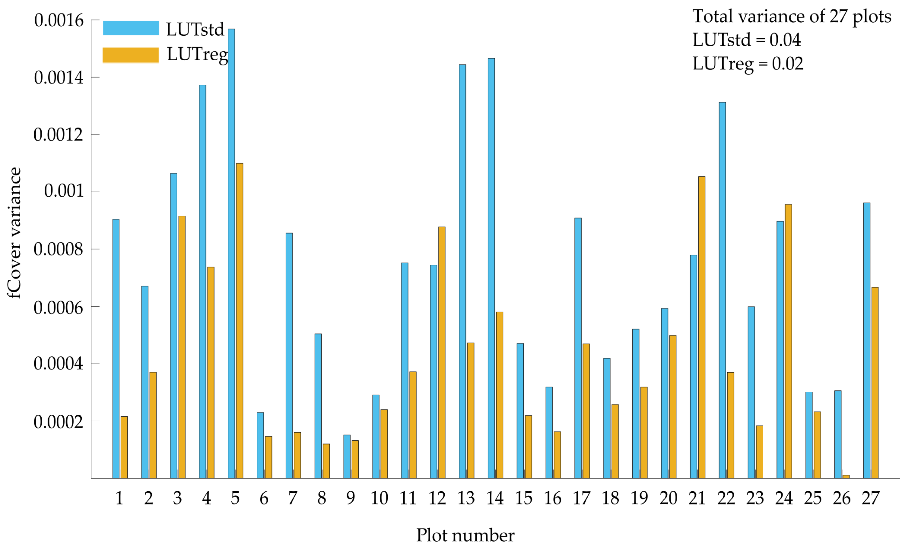
Both types of LUTs failed to accurately estimate the LCC variable using the SLC model (see Appendix A, Table A1). Other studies that have used the SLC model [33] or the PROSAIL model [12,13,24,36,39,59] have reported similar failures to accurately derive LCC. This issue might be caused by the limited range of LCC values in LUT and the uncertainty of using SPAD measurements [39]. For fCover, LUTreg could not improve the accuracy compared with LUTstd (R² = 0.69, NRMSE = 18.60% for LUTreg; R² = 0.70, NRMSE = 17.85% for LUTstd). However, the results of both scenarios revealed that the accuracy increased at high values of retrieved fCover (>0.4) and scattered points were distributed around the 1:1 regression line, comparable to Reference [69]. This result means that high values of fCover are indicative that the potato crop is homogeneous (fully covered by vegetation) in the horizontal direction. This observation is aligned with the assumption of the turbid medium of canopy RTMs. On the contrary, lower values of fCover (<0.4) were overestimated. This overestimation might be explained by the fact that non-leaf elements (i.e., stem, shoot and branch) that greatly affect the canopy reflectance are not reflected in the SLC model. In a study in Reference [70], when the vegetation cover was at a low level, the PROSAIL model overestimated the fCover for a corn crop, whose planting pattern is similar to that of the potato crop (discontinuous crops).

Calculating the variance also confirmed the improvement of the LAI estimate derived from LUTreg. This implies that the proposed method (Cholesky algorithm) reduced the inverse problem by decreasing the uncertainties of modelled spectra generated from LUT for each plot. However, compared with LUTstd, the percentage of variance for the Cv and fCover retrievals from LUTreg (50% for Cv and fCover, respectively) (Figure 8 and Figure 9) was not obvious, as in the case of LAI (60%) (Figure 7). The errors mainly came from the five plots of retrieved Cv from LUTreg. This is because these plots were not fully covered by the canopy (heterogeneous). In addition, the Cv parameter caused a nearly linear mixing of canopy and soil spectra, while LAI mainly modified the near-infrared spectrum, with deeper dips at high LAI. This likely induced problems related to the compensation effect between variables (LAI and Cv) since the fCover variable is a derived quantity from basic inputs (LAI, Cv, and the LIDF variables). The different combinations of Cv and LAI can produce the same value of fCover [33]. For instance, plots with high LAI and low Cv or vice versa increase the uncertainty in retrievals of fCover. Additionally, the plots that had low LAI and Cv were characterized by a high uncertainty in their corresponding estimations because of the contributions of the soil signature. Nevertheless, in plots with high values of LAI and Cv, the model represented more accurate estimations of fCover (corresponding to high values), indicating well-developed canopies.

Although LAI retrieval was improved by considering the variable correlations between LAI and fCover, there is still a need to examine the full correlation matrix among model variables to enhance fCover and CCC retrieval, as well. It is supposed that appraising the other correlations between free model variables (such as LAI–Cw/Cm/SM/LIDF and Cm–N/Cv) in LUT using the measured correlation variables will likely increase the reduction of the development of the unrealistic simulated reflectance produced by an unrealistic combination of input model variables. It is recommended that future research apply the presented method to different RTMs (i.e., PROSAIL, INFORM, or SCOPE) and to different areas at different scales in order to investigate the retrievals of various types of crops from different remote sensing products. To apply the proposed method for different observation dates or areas in a simple way an average correlation coefficient (between this range 0.65–0.90) can be used to improve the results instead of using correlation for a single date or area. However, for representing the actual situation for each observation data or area the Cholesky method can not be easily applicable in term of time calculations. Moreover, it is suggested to examine the given strategy with other inversion methods, such as OPT, Bayesian, and ANN.

5. Conclusions

This study presented the feasibility of using a Cholesky algorithm in the LUT-based inversion approach to improving predictions of the SLC model. To quantify vegetation attribute for 27 potato plots the LUT inversion approach was used as a robust and simple method using hyperspectral remote sensing data. Besides regularization techniques to optimize LUT inversion method, the incorporating known variable correlations were considered as an additional source of a priori information to avoid the generation of meaningless canopy spectra. The proposed method (Cholesky algorithm) utilizes the correlation between LAI and fCover that naturally exists in the study field to correlate the independent model variables LAI and Cv. Retrievals from the regularized LUT (LUTreg), which was modified by using known variable correlation were compared with the standard LUT (LUTstd).

The results revealed that LUTreg was appeared to be successful for improving the accuracy of retrieved LAI and CCC rather than LUTstd in term of R² and NRMSE%, because of reducing the probabilities of unrealistic combinations of model parameters. However, the estimated fCover was not improved by LUTreg that is due to the error of the estimated Cv. By calculating the variability of model predictions the estimated LAI (5.10) was remarkably decreased over 27 plots in LUTreg compared to LUTstd (12.10), while the estimated Cv and fCover from LUTreg were slightly decreased (0.10 and 0.02) as compared to LUTstd (0.20 and 0.04, respectively).

For further studies, two main issues could be addressed and taken into account. First, measuring the LIDF parameter and soil spectra in the field should be considered to increase the accuracy of fCover retrieval. Second, based on ground data sufficiency a full variance–covariance or correlation matrix of all involved variables of RTMs should be considered to implement the Cholesky algorithm efficiently for decreasing the uncertainties of retrievals especially for Cv, which is related to improve the accuracy of fCover variables.

References

1. Darvishzadeh, R.; Atzberger, C.; Skidmore, A.; Schlerf, M. Mapping grassland leaf area index with airborne hyperspectral imagery: A comparison study of statistical approaches and inversion of radiative transfer models. ISPRS J. Photogramm. Remote Sens. 2011, 66, 894–906. [Google Scholar] [CrossRef]
2. Jacquemoud, S.; Verhoef, W.; Baret, F.; Bacour, C.; Zarco-Tejada, P.J.; Asner, G.P.; François, C.; Ustin, S.L. PROSPECT+ SAIL models: A review of use for vegetation characterization. Remote Sens. Environ. 2009, 113, S56–S66. [Google Scholar] [CrossRef]
3. Xiao, Z.; Wang, T.; Liang, S.; Sun, R. Estimating the fractional vegetation cover from GLASS leaf area index product. Remote Sens. 2016, 8, 337. [Google Scholar] [CrossRef]
4. Mu, X.; Song, W.; Gao, Z.; McVicar, T.R.; Donohue, R.J.; Yan, G. Fractional vegetation cover estimation by using multi-angle vegetation index. Remote Sens. Environ. 2018, 216, 44–56. [Google Scholar] [CrossRef]
5. Zheng, G.; Moskal, L.M. Retrieving leaf area index (LAI) using remote sensing: Theories, methods and sensors. Sensors 2009, 9, 2719–2745. [Google Scholar] [CrossRef] [PubMed]
6. Li, X.; Liu, Q.; Yang, R.; Zhang, H.; Zhang, J.; Cai, E. The design and implementation of the leaf area index sensor. Sensors 2015, 15, 6250–6269. [Google Scholar] [CrossRef]
7. Li, Y.; Wang, H.; Li, X.B. Fractional vegetation cover estimation based on an improved selective endmember spectral mixture model. PLoS ONE 2015, 10, e0124608. [Google Scholar] [CrossRef]
8. Clevers, J.G.; Kooistra, L. Using hyperspectral remote sensing data for retrieving canopy chlorophyll and nitrogen content. IEEE J. Sel. Top. Appl. Earth Obs. Remote Sens. 2011, 5, 574–583. [Google Scholar] [CrossRef]
9. Clevers, J.; Kooistra, L.; Van Den Brande, M. Using Sentinel-2 data for retrieving LAI and leaf and canopy chlorophyll content of a potato crop. Remote Sens. 2017, 9, 405. [Google Scholar] [CrossRef]
10. Kooistra, L.; Clevers, J.G. Estimating potato leaf chlorophyll content using ratio vegetation indices. Remote Sens. Lett. 2016, 7, 611–620. [Google Scholar] [CrossRef]
11. Liu, D.; Yang, L.; Jia, K.; Liang, S.; Xiao, Z.; Wei, X.; Yao, Y.; Xia, M.; Li, Y. Global Fractional Vegetation Cover Estimation Algorithm for VIIRS Reflectance Data Based on Machine Learning Methods. Remote Sens. 2018, 10, 1648. [Google Scholar] [CrossRef]
12. Darvishzadeh, R.; Skidmore, A.; Schlerf, M.; Atzberger, C. Inversion of a radiative transfer model for estimating vegetation LAI and chlorophyll in a heterogeneous grassland. Remote Sens. Environ. 2008, 112, 2592–2604. [Google Scholar] [CrossRef]
13. Schlerf, M.; Atzberger, C. Inversion of a forest reflectance model to estimate structural canopy variables from hyperspectral remote sensing data. Remote Sens. Environ. 2006, 100, 281–294. [Google Scholar] [CrossRef]
14. Locherer, M.; Hank, T.; Danner, M.; Mauser, W. Retrieval of seasonal leaf area index from simulated EnMAP data through optimized LUT-based inversion of the PROSAIL model. Remote Sens. 2015, 7, 10321–10346. [Google Scholar] [CrossRef]
15. Weiss, M.; Baret, F.; Myneni, R.; Pragnère, A.; Knyazikhin, Y. Investigation of a model inversion technique to estimate canopy biophysical variables from spectral and directional reflectance data. Agric. Environ. 2000, 20, 3–22. [Google Scholar] [CrossRef]
16. Houborg, R.; Soegaard, H.; Boegh, E. Combining vegetation index and model inversion methods for the extraction of key vegetation biophysical parameters using Terra and Aqua MODIS reflectance data. Remote Sens. Environ. 2007, 106, 39–58. [Google Scholar] [CrossRef]
17. Yebra, M.; Chuvieco, E. Linking ecological information and radiative transfer models to estimate fuel moisture content in the Mediterranean region of Spain: Solving the ill-posed inverse problem. Remote Sens. Environ. 2009, 113, 2403–2411. [Google Scholar] [CrossRef]
18. Sehgal, V.K.; Chakraborty, D.; Sahoo, R.N. Inversion of radiative transfer model for retrieval of wheat biophysical parameters from broadband reflectance measurements. Inf. Process. Agric. 2016, 3, 107–118. [Google Scholar] [CrossRef]
19. Qin, J.; Liang, S.; Li, X.; Wang, J. Development of the adjoint model of a canopy radiative transfer model for sensitivity study and inversion of leaf area index. IEEE Trans. Geosci. Remote Sens. 2008, 46, 2028–2037. [Google Scholar] [CrossRef]
20. Combal, B.; Baret, F.; Weiss, M.; Trubuil, A.; Mace, D.; Pragnere, A.; Myneni, R.; Knyazikhin, Y.; Wang, L. Retrieval of canopy biophysical variables from bidirectional reflectance: Using prior information to solve the ill-posed inverse problem. Remote Sens. Environ. 2003, 84, 1–15. [Google Scholar] [CrossRef]
21. Berger, K.; Atzberger, C.; Danner, M.; D’Urso, G.; Mauser, W.; Vuolo, F.; Hank, T. Evaluation of the PROSAIL model capabilities for future hyperspectral model environments: A review study. Remote Sens. 2018, 10, 85. [Google Scholar] [CrossRef]
22. Verhoef, W.; Bach, H. Coupled soil–leaf-canopy and atmosphere radiative transfer modeling to simulate hyperspectral multi-angular surface reflectance and TOA radiance data. Remote Sens. Environ. 2007, 109, 166–182. [Google Scholar] [CrossRef]
23. Levashova, N.; Lukyanenko, D.; Mukhartova, Y.; Olchev, A. Application of a Three-Dimensional Radiative Transfer Model to Retrieve the Species Composition of a Mixed Forest Stand from Canopy Reflected Radiation. Remote Sens. 2018, 10, 1661. [Google Scholar] [CrossRef]
24. Mousivand, A.; Menenti, M.; Gorte, B.; Verhoef, W. Multi-temporal, multi-sensor retrieval of terrestrial vegetation properties from spectral–directional radiometric data. Remote Sens. Environ. 2015, 158, 311–330. [Google Scholar] [CrossRef]
25. Jacquemoud, S.; Bacour, C.; Poilve, H.; Frangi, J.P. Comparison of four radiative transfer models to simulate plant canopies reflectance: Direct and inverse mode. Remote Sens. Environ. 2000, 74, 471–481. [Google Scholar] [CrossRef]
26. Jacquemoud, S.; Baret, F.; Andrieu, B.; Danson, F.; Jaggard, K. Extraction of vegetation biophysical parameters by inversion of the PROSPECT+ SAIL models on sugar beet canopy reflectance data. Application to TM and AVIRIS sensors. Remote Sens. Environ. 1995, 52, 163–172. [Google Scholar] [CrossRef]
27. Fang, H.; Liang, S. A hybrid inversion method for mapping leaf area index from MODIS data: Experiments and application to broadleaf and needleleaf canopies. Remote Sens. Environ. 2005, 94, 405–424. [Google Scholar] [CrossRef]
28. Walthall, C.; Dulaney, W.; Anderson, M.; Norman, J.; Fang, H.; Liang, S. A comparison of empirical and neural network approaches for estimating corn and soybean leaf area index from Landsat ETM+ imagery. Remote Sens. Environ. 2004, 92, 465–474. [Google Scholar] [CrossRef]
29. Weiss, M.; Baret, F. Evaluation of canopy biophysical variable retrieval performances from the accumulation of large swath satellite data. Remote Sens. Environ. 1999, 70, 293–306. [Google Scholar] [CrossRef]
30. Fang, H.; Liang, S.; Kuusk, A. Retrieving leaf area index using a genetic algorithm with a canopy radiative transfer model. Remote Sens. Environ. 2003, 85, 257–270. [Google Scholar] [CrossRef]
31. Durbha, S.S.; King, R.L.; Younan, N.H. Support vector machines regression for retrieval of leaf area index from multiangle imaging spectroradiometer. Remote Sens. Environ. 2007, 107, 348–361. [Google Scholar] [CrossRef]
32. Qu, Y.; Wang, J.; Wan, H.; Li, X.; Zhou, G. A Bayesian network algorithm for retrieving the characterization of land surface vegetation. Remote Sens. Environ. 2008, 112, 613–622. [Google Scholar] [CrossRef]
33. Laurent, V.C.; Verhoef, W.; Damm, A.; Schaepman, M.E.; Clevers, J.G. A Bayesian object-based approach for estimating vegetation biophysical and biochemical variables from APEX at-sensor radiance data. Remote Sens. Environ. 2013, 139, 6–17. [Google Scholar] [CrossRef]
34. Verrelst, J.; Camps-Valls, G.; Muñoz-Marí, J.; Rivera, J.P.; Veroustraete, F.; Clevers, J.G.; Moreno, J. Optical remote sensing and the retrieval of terrestrial vegetation bio-geophysical properties—A review. ISPRS J. Photogramm. Remote Sens. 2015, 108, 273–290. [Google Scholar] [CrossRef]
35. Atzberger, C. Object-based retrieval of biophysical canopy variables using artificial neural nets and radiative transfer models. Remote Sens. Environ. 2004, 93, 53–67. [Google Scholar] [CrossRef]
36. Baret, F.; Jacquemoud, S. Modeling canopy spectral properties to retrieve biophysical and biochemical characteristics. In Imaging Spectrometry—A Tool for Environmental Observations; Springer: Dordrecht, The Netherlands, 1994; pp. 145–167. [Google Scholar]
37. Duan, S.B.; Li, Z.L.; Wu, H.; Tang, B.H.; Ma, L.; Zhao, E.; Li, C. Inversion of the PROSAIL model to estimate leaf area index of maize, potato, and sunflower fields from unmanned aerial vehicle hyperspectral data. Int. J. Appl. Earth Obs. Geoinf. 2014, 26, 12–20. [Google Scholar] [CrossRef]
38. Hadamard, J. Sur les problemes aux derivees partielles et leur signification physique. Princet. Univ. Bull. 1902, 13, 49–52. [Google Scholar]
39. Roosjen, P.P.; Brede, B.; Suomalainen, J.M.; Bartholomeus, H.M.; Kooistra, L.; Clevers, J.G. Improved estimation of leaf area index and leaf chlorophyll content of a potato crop using multi-angle spectral data–potential of unmanned aerial vehicle imagery. Int. J. Appl. Earth Obs. Geoinf. 2018, 66, 14–26. [Google Scholar] [CrossRef]
40. Leonenko, G.; Los, S.O.; North, P.R.J. Statistical Distances and Their Applications to Biophysical Parameter Estimation: Information Measures, M-Estimates, and Minimum Contrast Methods. Remote Sens. 2013, 5, 1355–1388. [Google Scholar] [CrossRef] [Green Version]
41. Leonenko, G.; Los, S.; North, P. Retrieval of leaf area index from MODIS surface reflectance by model inversion using different minimization criteria. Remote Sens. Environ. 2013, 139, 257–270. [Google Scholar] [CrossRef]
42. Lavergne, T.; Kaminski, T.; Pinty, B.; Taberner, M.; Gobron, N.; Verstraete, M.M.; Vossbeck, M.; Widlowski, J.L.; Giering, R. Application to MISR land products of an RPV model inversion package using adjoint and Hessian codes. Remote Sens. Environ. 2007, 107, 362–375. [Google Scholar] [CrossRef]
43. Bacour, C.; Jacquemoud, S.; Vogt, P.; Hosgood, B.; Andreoli, G.; Frangi, J.P. Optimal sampling configurations for the estimation of canopy properties from BRDF data acquired with the EGO/JRC. In Proceedings of the 8th International Symposium Physical Measurements & Signatures in Remote Sensing, Aussois, France, 8–12 January 2001; Available online: https://www.semanticscholar.org/paper/OPTIMAL-SAMPLING-CONFIGURATIONS-FOR-THE-ESTIMATION-Bacour-Jacquemoud/41f35a794f543e1a0e78e3bb97f2b8fc85dac864 (accessed on 3 January 2018).
44. Baret, F.; Houles, V.; Guérif, M. Quantification of plant stress using remote sensing observations and crop models: the case of nitrogen management. J. Exp. Bot. 2007, 58, 869–880. [Google Scholar] [CrossRef] [Green Version]
45. Koetz, B.; Baret, F.; Poilvé, H.; Hill, J. Use of coupled canopy structure dynamic and radiative transfer models to estimate biophysical canopy characteristics. Remote Sens. Environ. 2005, 95, 115–124. [Google Scholar] [CrossRef]
46. Richter, K.; Timmermans, W. Physically based retrieval of crop characteristics for improved water use estimates. Hydrol. Earth Syst. Sci. 2009, 13, 663–674. [Google Scholar] [CrossRef] [Green Version]
47. Quan, X.; He, B.; Li, X. A Bayesian network-based method to alleviate the ill-posed inverse problem: A case study on leaf area index and canopy water content retrieval. IEEE Trans. Geosci. Remote Sens. 2015, 53, 6507–6517. [Google Scholar] [CrossRef]
48. Parker, M. Chapter 13—Matrix Inversion. In Digital Signal Processing 101, 2nd ed.; Cambridge University Press: Cambridge, UK, 2005; pp. 149–162. [Google Scholar]
49. Shi, W.; Guo, Y.F. Incomplete Cholesky decomposition based kernel principal component analysis for large-scale data set. In Proceedings of the 2010 International Joint Conference on Neural Networks (IJCNN), Barcelona, Spain, 18–23 July 2010. [Google Scholar]
50. Sabino, P. Monte Carlo methods and path-generation techniques for pricing multi-asset path-dependent options. arXiv 2007, arXiv:0710.0850. [Google Scholar] [CrossRef] [Green Version]
51. Liu, J.W. An adaptive general sparse out-of-core Cholesky factorization scheme. SIAM J. Sci. Stat. Comput. 1987, 8, 585–599. [Google Scholar] [CrossRef]
52. Camps-Valls, G.; Muñoz-Marí, J.; Gómez-Chova, L.; Richter, K.; Calpe-Maravilla, J. Biophysical parameter estimation with a semisupervised support vector machine. IEEE Geosci. Remote Sens. Lett. 2009, 6, 248–252. [Google Scholar] [CrossRef]
53. Pasolli, L.; Melgani, F.; Blanzieri, E. Gaussian process regression for estimating chlorophyll concentration in subsurface waters from remote sensing data. IEEE Geosci. Remote Sens. Lett. 2010, 7, 464–468. [Google Scholar] [CrossRef]
54. Hueni, A.; Bialek, A. Cause, effect, and correction of field spectroradiometer interchannel radiometric steps. IEEE J. Sel. Top. Appl. Earth Obs. Remote Sens. 2017, 10, 1542–1551. [Google Scholar] [CrossRef]
55. Uddling, J.; Gelang-Alfredsson, J.; Piikki, K.; Pleijel, H. Evaluating the relationship between leaf chlorophyll concentration and SPAD-502 chlorophyll meter readings. Photosynth. Res. 2007, 91, 37–46. [Google Scholar] [CrossRef] [PubMed]
56. Hapke, B. Bidirectional reflectance spectroscopy: 1. Theory. J. Geophys. Res. Solid Earth 1981, 86, 3039–3054. [Google Scholar] [CrossRef]
57. Jacquemoud, S.; Baret, F. PROSPECT: A model of leaf optical properties spectra. Remote Sens. Environ. 1990, 34, 75–91. [Google Scholar] [CrossRef]
58. Tong, A. Estimating Grassland Chlorophyll Content for a Mixed Grassland: Exploring the Performance of the Empirical-Statistical and the Physical Modeling Approach. Master’s Thesis, 2014; pp. 62–69. Available online: http://hdl.handle.net/1807/82667 (accessed on 4 November 2018).
59. Botha, E.J.; Leblon, B.; Zebarth, B.; Watmough, J. Non-destructive estimation of potato leaf chlorophyll from canopy hyperspectral reflectance using the inverted PROSAIL model. Int. J. Appl. Earth Obs. Geoinf. 2007, 9, 360–374. [Google Scholar] [CrossRef]
60. Casa, R.; Jones, H. Retrieval of crop canopy properties: A comparison between model inversion from hyperspectral data and image classification. Int. J. Remote Sens. 2004, 25, 1119–1130. [Google Scholar] [CrossRef]
61. Edlin, R.; McCabe, C.; Hulme, C.; Hall, P.; Wright, J. Correlated Parameters and the Cholesky Decomposition. In Cost Effectiveness Modelling for Health Technology Assessment; ADIS: Cham, Switzerland, 2015; pp. 119–132. [Google Scholar]
62. Higham, N.J. Cholesky factorization. Wiley Interdiscip. Rev. 2009, 1, 251–254. [Google Scholar] [CrossRef]
63. Yu, H.; Chung, C.; Wong, K.; Lee, H.; Zhang, J. Probabilistic load flow evaluation with hybrid latin hypercube sampling and cholesky decomposition. IEEE Trans. Power Syst. 2009, 24, 661–667. [Google Scholar] [CrossRef]
64. Vuolo, F.; Atzberger, C.; Richter, K.; D’Urso, G.; Dash, J. Retrieval of Biophysical Vegetation Products from RapidEye Imagery. Available online: http://publications.jrc.ec.europa.eu/repository/handle/JRC55768 (accessed on 1 January 2018).
65. Rivera, J.; Verrelst, J.; Leonenko, G.; Moreno, J. Multiple cost functions and regularization options for improved retrieval of leaf chlorophyll content and LAI through inversion of the PROSAIL model. Remote Sens. 2013, 5, 3280–3304. [Google Scholar] [CrossRef] [Green Version]
66. Darvishzadeh, R.; Matkan, A.A.; Dashti Ahangar, A. Inversion of a Radiative Transfer Model for Estimation of Rice Canopy Chlorophyll Content Using a Lookup-Table Approach. IEEE J. Sel. Top. Appl. Earth Obs. Remote Sens. 2012, 5, 1222–1230. [Google Scholar] [CrossRef] [Green Version]
67. He, W.; Yang, H.; Pan, J.; Xu, P. Exploring optimal design of look-up table for PROSAIL model inversion with multi-angle MODIS data. In Land Surface Remote Sensing; International Society for Optics and Photonics: Bellingham, WA, USA, 2012; Volume 8524, p. 852420. [Google Scholar]
68. D’Urso, G.; Dini, L.; Vuolo, F.; Alonso, L.; Guanter, L. Retrieval of leaf area index by inverting hyperspectral multiangular CHRIS PROBA data from SPARC 2003. In Proceedings of the 2nd CHRIS Proba Workshop, Frascati, Italy, 28–30 April 2004; Volume 28, pp. 58–63. [Google Scholar]
69. Jia, K.; Liang, S.; Gu, X.; Baret, F.; Wei, X.; Wang, X.; Yao, Y.; Yang, L.; Li, Y. Fractional vegetation cover estimation algorithm for Chinese GF-1 wide field view data. Remote Sens. Environ. 2016, 177, 184–191. [Google Scholar] [CrossRef]
70. Ding, Y.; Zhang, H.; Li, Z.; Xin, X.; Zheng, X.; Zhao, K. Comparison of fractional vegetation cover estimations using dimidiate pixel models and look-up table inversions of the PROSAIL model from Landsat 8 OLI data. J. Appl. Remote Sens. 2016, 10, 036022. [Google Scholar] [CrossRef]
Figure 1. The layout of the experimental plots: (A) a map of the study area (left side) in which the star indicates the position of the study site; (B) the arrangement of the nitrogen fertilization experiment (the lower-right side); and (C) the plot design for in situ measurements (the upper right.)
Remotesensing 11 02681 g001
Figure 2. Relationships between LAI and Cv variables using forward simulations (a) without variable correlation and (b) with variable correlation using the Cholesky method.
Remotesensing 11 02681 g002
Figure 3. Comparison between measured (black) and simulated (red) spectra for four types of leaf inclination distribution functions (LIDFs) and four selected potato plots (cases) to identify the LIDF type that best represents potato.
Remotesensing 11 02681 g003
Figure 4. Relation between estimated LAI and Cv from LUTstd (a) and LUTreg (b).
Remotesensing 11 02681 g004
Figure 5. The estimated LAI from LUTstd (a) and LUTreg (b).
Remotesensing 11 02681 g005
Figure 6. The estimated fCover from LUTstd (a) and LUTreg (b).
Remotesensing 11 02681 g006
Figure 7. The magnitude of LAI variation across 27 potato plots obtained from both types of LUTs.
Remotesensing 11 02681 g007
Figure 8. The magnitude of Cv variation across 27 potato plots obtained from both types of LUTs.
Remotesensing 11 02681 g008
Figure 9. The magnitude of fCover variation across 27 potato plots obtained from both types of LUTs.
Remotesensing 11 02681 g009