High-Resolution Sea Surface Temperature Retrieval from Landsat 8 OLI/TIRS Data at Coastal Regions


Abstract
:
1. Introduction
2. Data
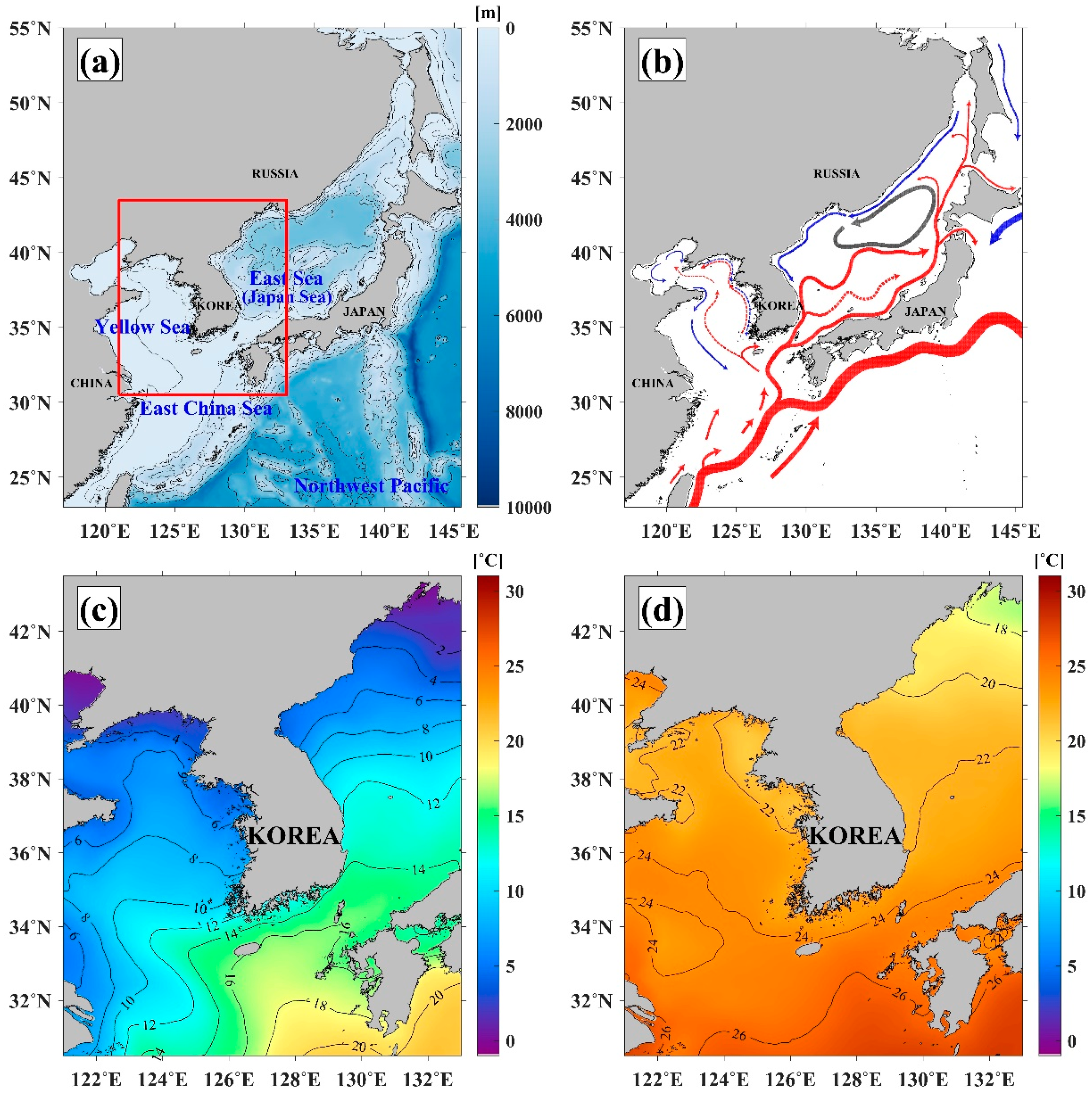
2.1. Study Area
2.2. Satellite Data
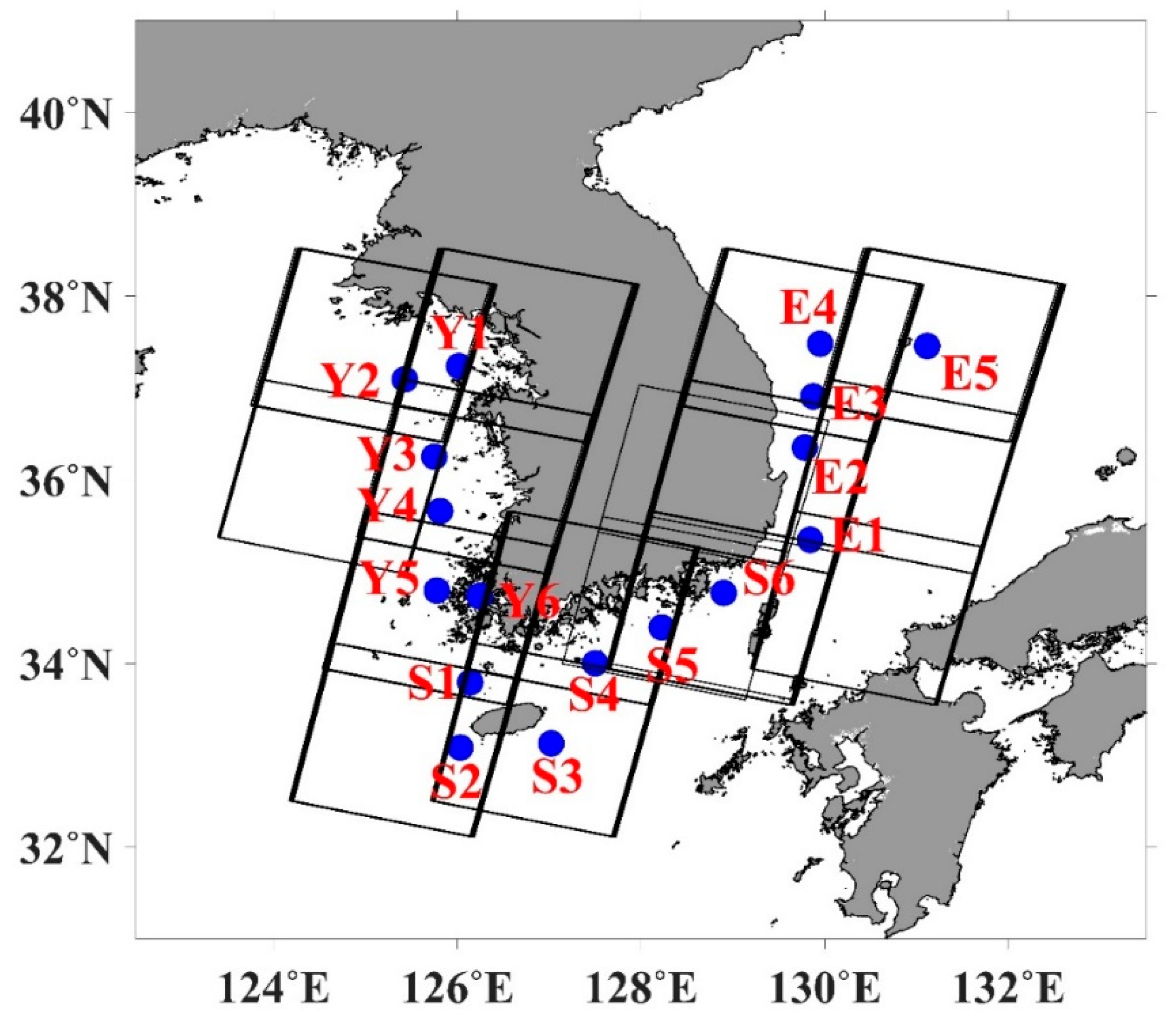
2.3. In-Situ Measurements
2.4. Daily SST Data
3. Methods
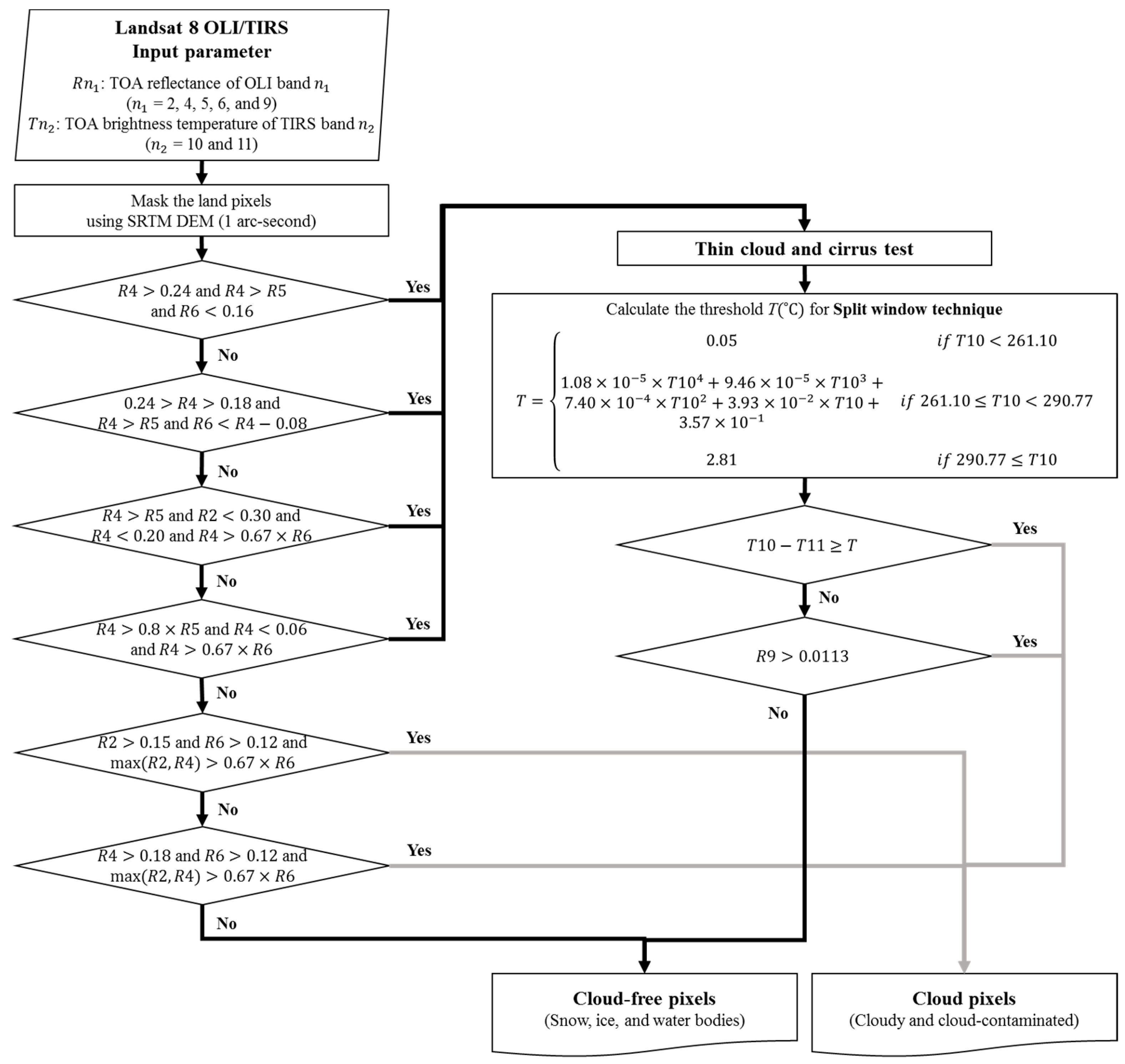
3.1. Removal of Cloud-Contaminated Pixels
3.2. SST Retrieval Algorithms
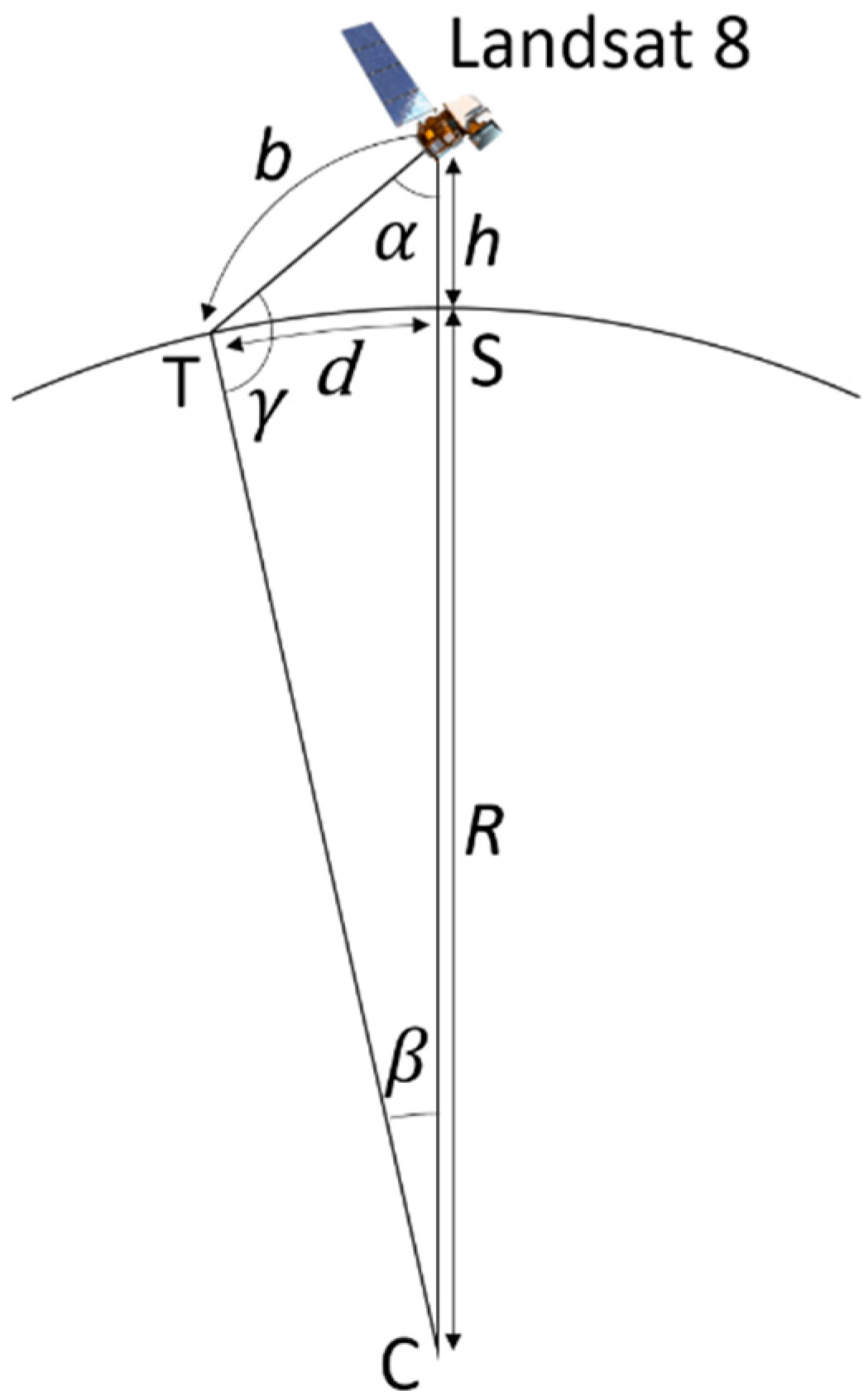
3.3. Calculation of Satellite Zenith Angle
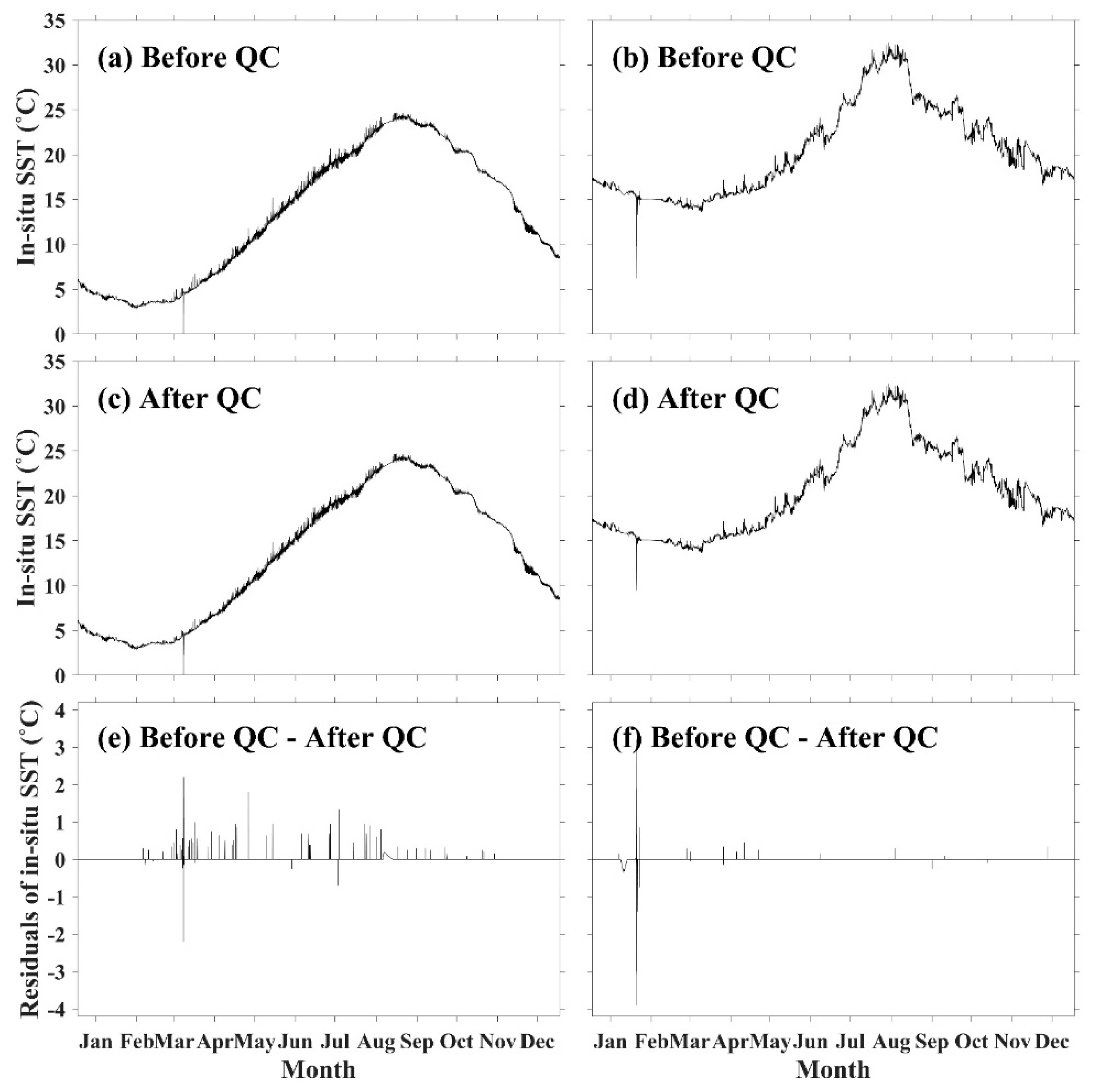
3.4. Quality Control of In-Situ Measurements
4. Results
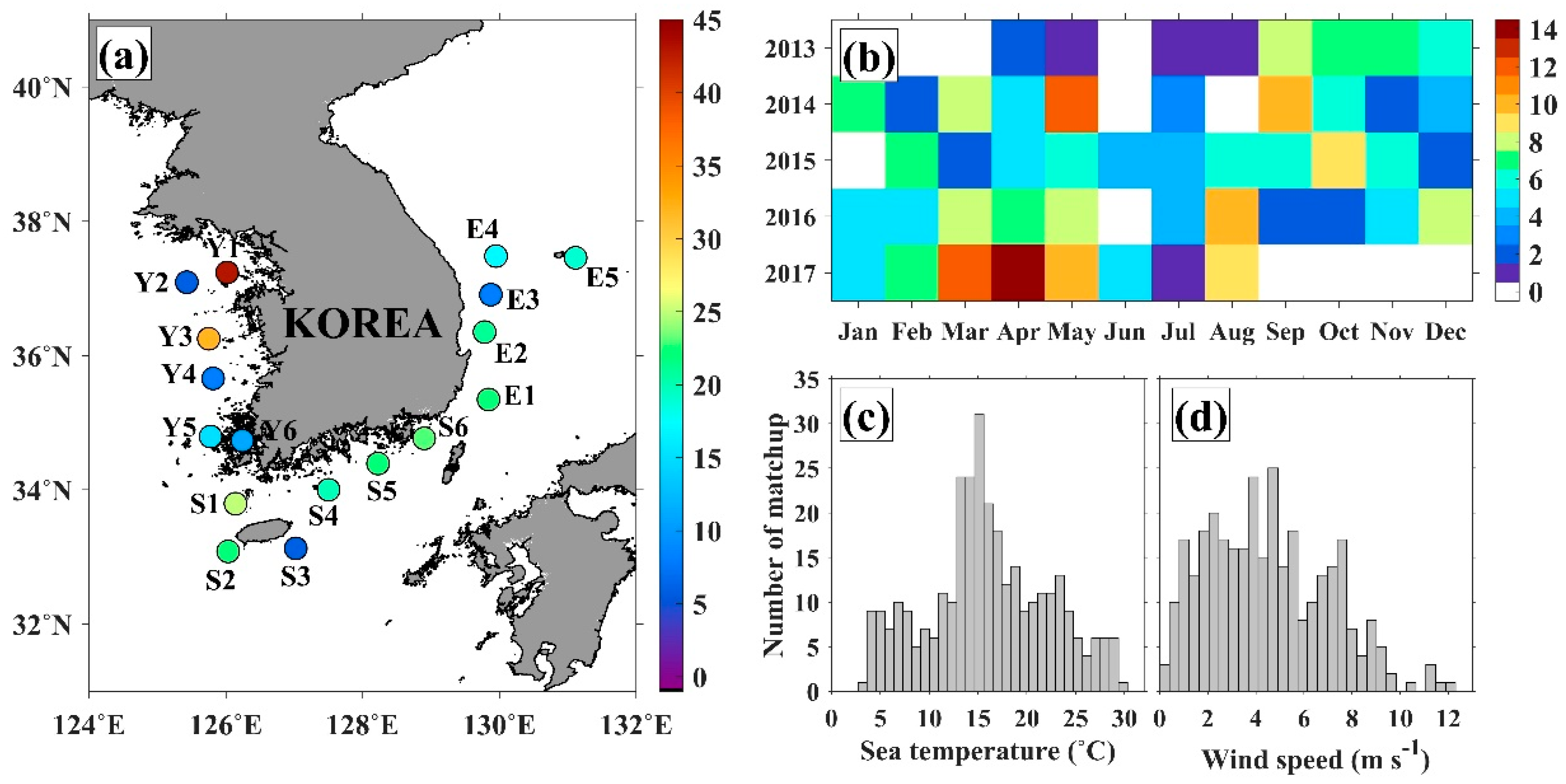
4.1. Matchup Data
4.2. Derivation of SST Coefficients
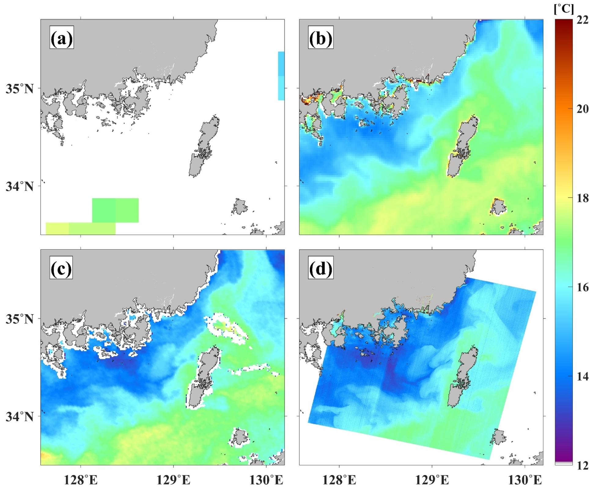
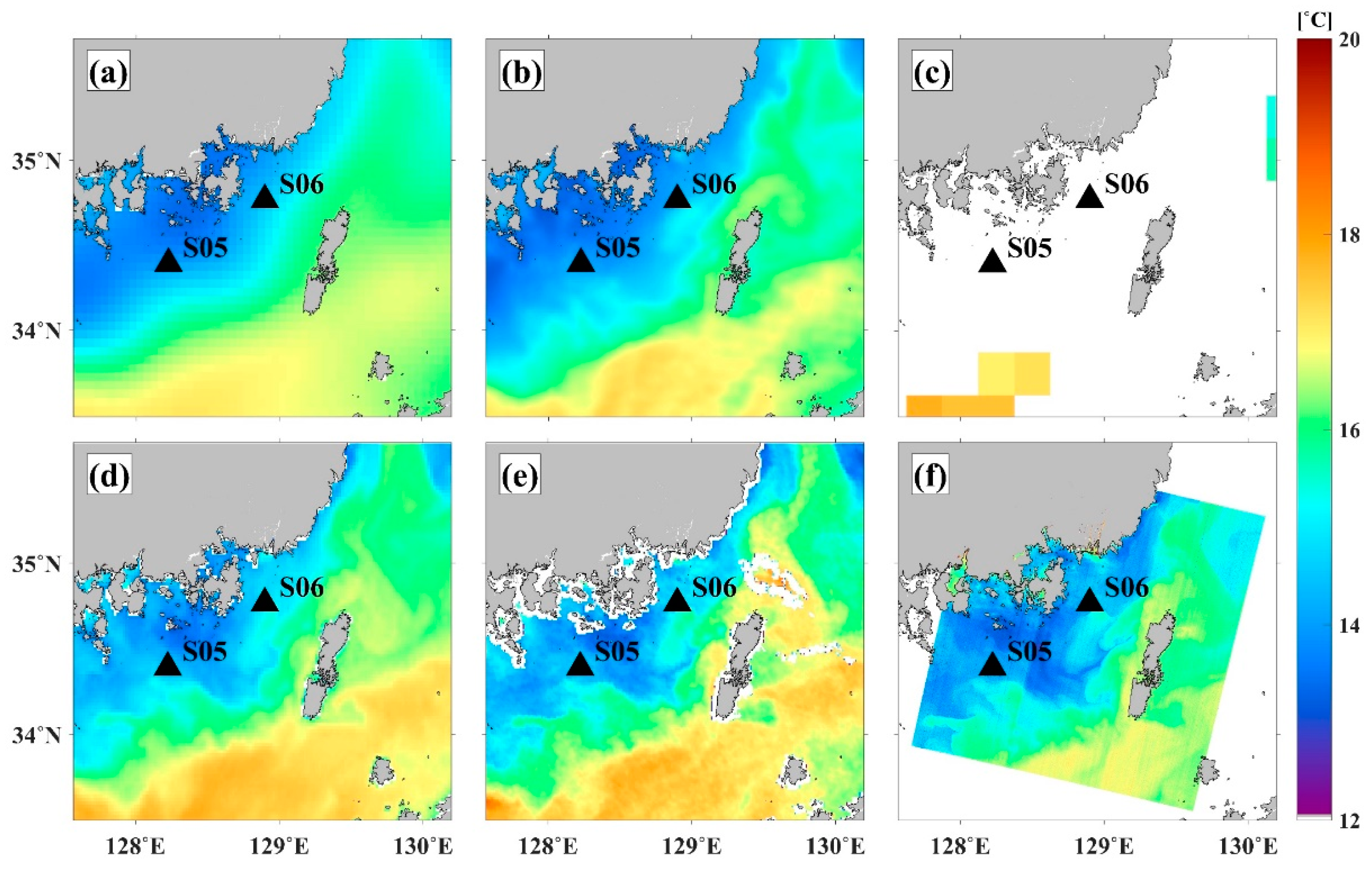
4.3. High-Resolution SST
5. Discussion
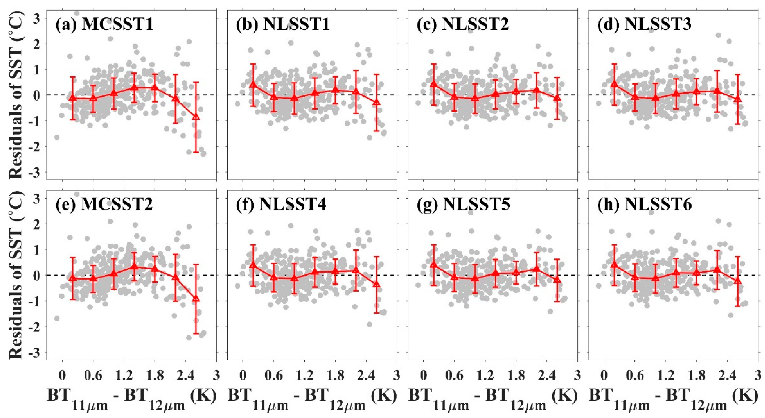
5.1. Effect of Atmospheric Moisture
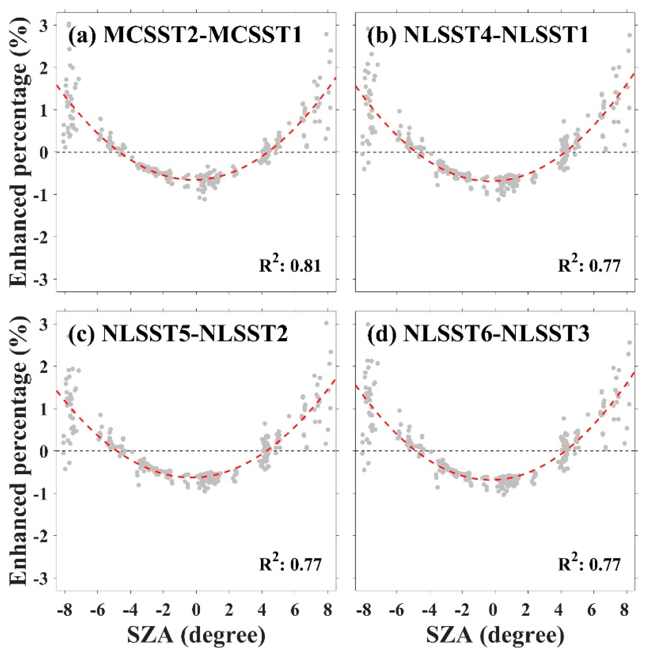
5.2. Effect of SZA
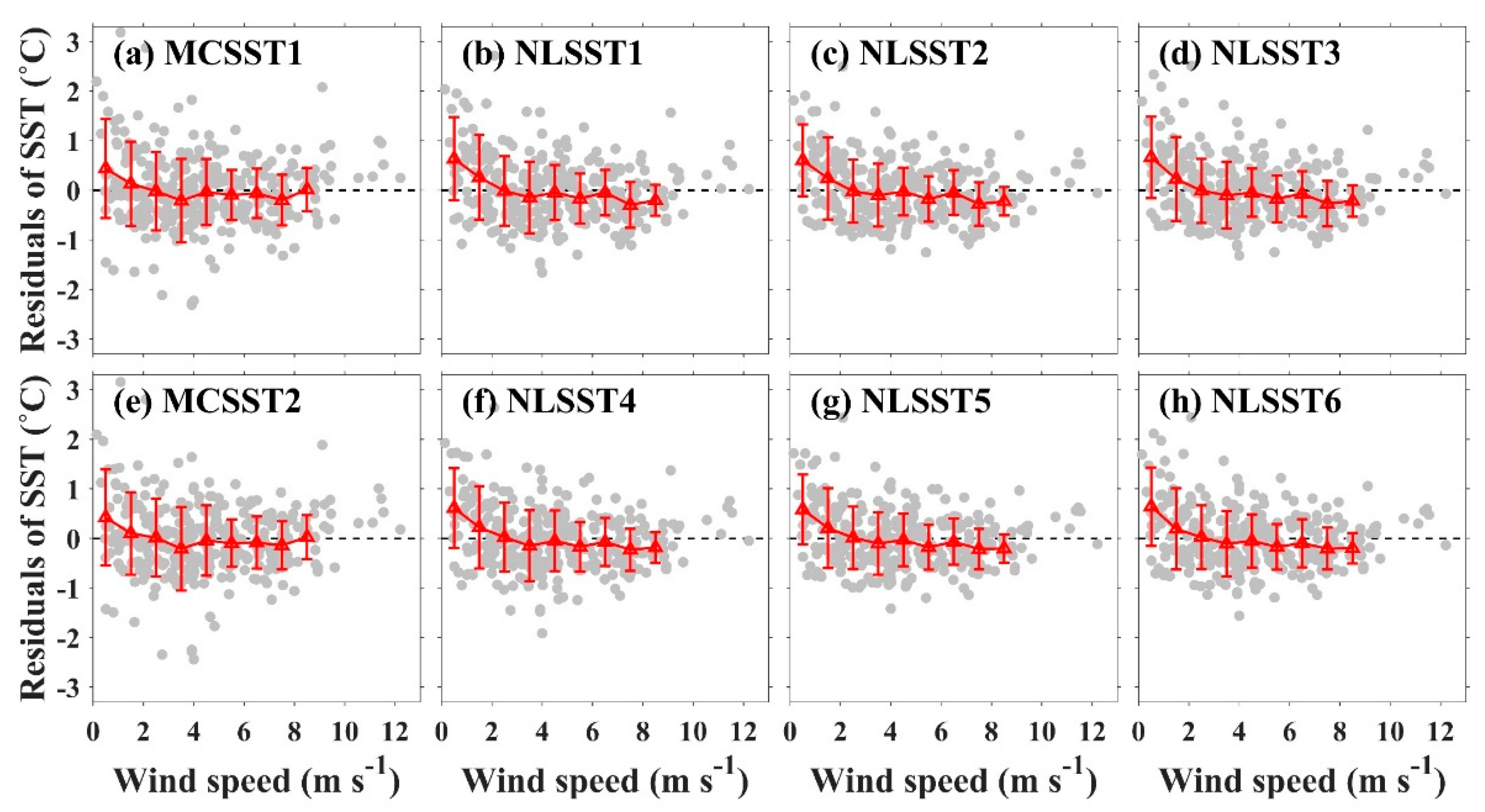
5.3. Effect of Wind Speed
6. Summary and Conclusions
Author Contributions
Funding
Acknowledgments
Conflicts of Interest
References
- Corlett, G.K.; Barton, I.J.; Donlon, C.J.; Edwards, M.C.; Good, S.A.; Horrocks, L.A.; Llewellyn-Jones, D.T.; Merchant, C.J.; Minnett, P.J.; Nightingale, T.J.; et al. The accuracy of SST retrievals from AATSR: An initial assessment through geophysical validation against in situ radiometers, buoys and other SST data sets. Adv. Space Res. 2006, 37, 764–769. [Google Scholar] [CrossRef]
- Dash, P.; Ignatov, A.; Kihai, Y.; Sapper, J. The SST quality monitor (SQUAM). J. Atmos. Ocean. Technol. 2010, 27, 1899–1917. [Google Scholar] [CrossRef]
- Ullman, D.S.; Cornillon, P.C. Evaluation of front detection methods for satellite-derived SST data using in situ observations. J. Atmos. Ocean. Technol. 2000, 17, 1667–1675. [Google Scholar] [CrossRef]
- Park, K.A.; Chung, J.Y.; Kim, K. Sea surface temperature fronts in the East (Japan) Sea and temporal variations. Geophys. Res. Lett. 2004, 31. [Google Scholar] [CrossRef]
- Park, K.A.; Cornillon, P.; Codiga, D.L. Modification of surface winds near ocean fronts: Effects of Gulf Stream rings on scatterometer (QuikSCAT, NSCAT) wind observations. J. Geophys. Res. 2006, 111. [Google Scholar] [CrossRef]
- O’Neill, L.W.; Chelton, D.B.; Esbensen, S.K.; Wentz, F.J. High-resolution satellite measurements of the atmospheric boundary layer response to SST variations along the Agulhas Return Current. J. Clim. 2005, 18, 2706–2723. [Google Scholar] [CrossRef]
- Park, K.-A.; Cornilon, P.C. Stability-induced modification of sea surface winds over Gulf Stream rings. Geophys. Res. Lett. 2002, 29. [Google Scholar] [CrossRef]
- Casey, K.S.; Cornillon, P. Global and regional sea surface temperature trends. J. Clim. 2001, 14, 3801–3818. [Google Scholar] [CrossRef]
- Minnett, P.J.; Corlett, G.K. A pathway to generating Climate Data Records of sea-surface temperature from satellite measurements. Deep Sea Res. II 2012, 77, 44–51. [Google Scholar] [CrossRef]
- Merchant, C.J.; Embury, O.; Rayner, N.A.; Berry, D.I.; Corlett, G.K.; Lean, K.; Veal, K.L.; Kent, E.C.; Llewellyn-Jones, D.T.; Remedios, J.J.; et al. A 20 year independent record of sea surface temperature for climate from Along-Track Scanning Radiometers. J. Geophys. Res. 2012, 117. [Google Scholar] [CrossRef]
- Anding, D.; Kauth, R. Estimation of sea surface temperature from space. Remote Sens. Environ. 1970, 1, 217–220. [Google Scholar] [CrossRef]
- Prabhakara, C.; Dalu, G.; Kunde, V.G. Estimation of sea surface temperature from remote sensing in the 11-to 13-μm window region. J. Geophys. Res. 1974, 79, 5039–5044. [Google Scholar] [CrossRef]
- McMillin, L.M. Estimation of sea surface temperature from two infrared window measurements with different absorptions. J. Geophys. Res. 1975, 80, 5113–5117. [Google Scholar] [CrossRef]
- Bernstein, R.L. Sea surface temperature estimation using the NOAA 6 satellite advanced very high resolution radiometer. J. Geophys. Res. 1982, 87, 9455–9465. [Google Scholar] [CrossRef]
- McMillin, L.M.; Crosby, D.S. Theory and validation of the multiple window sea surface temperature technique. J. Geophys. Res. 1984, 89, 3655–3661. [Google Scholar] [CrossRef]
- McClain, E.P.; Pichel, W.G.; Walton, C.C. Comparative performance of AVHRR-based multichannel sea surface temperatures. J. Geophys. Res. 1985, 90, 11587–11601. [Google Scholar] [CrossRef]
- Walton, C.C. Nonlinear multichannel algorithms for estimating sea surface temperature with AVHRR satellite data. J. Appl. Meteorol. 1988, 27, 115–124. [Google Scholar] [CrossRef]
- Walton, C.C.; Pichel, W.G.; Sapper, J.F.; May, D.A. The development and operational application of nonlinear algorithms for the measurement of sea surface temperatures with the NOAA polar-orbiting environmental satellites. J. Geophys. Res. 1998, 103, 27999–28012. [Google Scholar] [CrossRef]
- Kilpatrick, K.A.; Podesta, G.P.; Evans, R. Overview of the NOAA/NASA advanced very high resolution radiometer Pathfinder algorithm for sea surface temperature and associated matchup database. J. Geophys. Res. 2001, 106, 9179–9197. [Google Scholar] [CrossRef]
- Li, X.; Pichel, W.; Maturi, E.; Clemente-Colon, P.; Sapper, J. Deriving the operational nonlinear multichannel sea surface temperature algorithm coefficients for NOAA-15 AVHRR/3. Int. J. Remote Sens. 2001, 22, 699–704. [Google Scholar] [CrossRef]
- May, D.A.; Osterman, W.O. Satellite-derived sea surface temperatures: Evaluation of GOES-8 and GOES-9 multispectral imager retrieval accuracy. J. Atmos. Ocean. Technol. 1998, 15, 788–797. [Google Scholar] [CrossRef]
- Donlon, C.J.; Castro, S.L.; Kaye, A. Aircraft validation of ERS-1 ATSR and NOAA-14 AVHRR sea surface temperature measurements. Int. J. Remote Sens. 1999, 20, 3503–3513. [Google Scholar] [CrossRef]
- Kumar, A.; Minnett, P.; Podestá, G.; Evans, R.; Kilpatrick, K. Analysis of Pathfinder SST algorithm for global and regional conditions. J. Earth Syst. Sci. 2000, 109, 395–405. [Google Scholar] [CrossRef]
- Minnett, P.J.; Evans, R.H.; Kearns, E.J.; Brown, O.B. Sea-surface temperature measured by the Moderate Resolution Imaging Spectroradiometer (MODIS). In Proceedings of the IEEE International Geoscience and Remote Sensing Symposium (IGARSS), Toronto, ON, Canada, 24–28 June 2002. [Google Scholar]
- Park, K.A.; Lee, E.Y.; Li, X.; Chung, S.R.; Sohn, E.H.; Hong, S. NOAA/AVHRR sea surface temperature accuracy in the East/Japan Sea. Int. J. Digit. Earth 2015, 8, 784–804. [Google Scholar] [CrossRef]
- Hao, Y.; Cui, T.; Singh, V.P.; Zhang, J.; Yu, R.; Zhang, Z. Validation of MODIS Sea Surface Temperature Product in the Coastal Waters of the Yellow Sea. IEEE J. Sel. Top. Appl. Earth Obs. Remote Sens. 2017, 10, 1667–1680. [Google Scholar] [CrossRef]
- Merchant, C.J.; Le Borgne, P.; Marsouin, A.; Roquet, H. Optimal estimation of sea surface temperature from split-window observations. Remote Sens. Environ. 2008, 112, 2469–2484. [Google Scholar] [CrossRef]
- Merchant, C.J.; Harris, A.R.; Roquet, H.; Le Borgne, P. Retrieval characteristics of non-linear sea surface temperature from the Advanced Very High Resolution Radiometer. Geophys. Res. Lett. 2009, 36. [Google Scholar] [CrossRef]
- Petrenko, B.; Ignatov, A.; Kihai, Y.; Stroup, J.; Dash, P. Evaluation and selection of SST regression algorithms for JPSS VIIRS. J. Geophys. Res. 2014, 119, 4580–4599. [Google Scholar] [CrossRef]
- Cracknell, A.P. Remote sensing techniques in estuaries and coastal zones an update. Int. J. Remote Sens. 1999, 20, 485–496. [Google Scholar] [CrossRef]
- Thomas, A.; Byrne, D.; Weatherbee, R. Coastal sea surface temperature variability from Landsat infrared data. Remote Sens. Environ. 2002, 81, 262–272. [Google Scholar] [CrossRef]
- Lira, C.; Taborda, R. Advances in applied remote sensing to coastal environments using free satellite imagery. In Remote Sensing and Modeling; Springer: Berlin/Heidelberg, Germany, 2014; pp. 77–102. [Google Scholar]
- Thomas, L.N.; Tandon, A.; Mahadevan, A. Submesoscale Processes and Dynamics. In Ocean Modeling in an Eddying Regime; American Geophysical Union: Washington, DC, USA, 2008; pp. 17–23. [Google Scholar]
- Castro, S.; Emery, W.; Wick, G.; Tandy, W. Submesoscale sea surface temperature variability from UAV and satellite measurements. Remote Sens. 2017, 9, 1089. [Google Scholar] [CrossRef] [Green Version]
- Gohin, F.; Langlois, G. Using geostatistics to merge in situ measurements and remotely-sensed observations of sea surface temperature. Int. J. Remote Sens. 1993, 14, 9–19. [Google Scholar] [CrossRef]
- Emery, W.J.; Castro, S.; Wick, G.A.; Schluessel, P.; Donlon, C. Estimating sea surface temperature from infrared satellite and in situ temperature data. Bull. Am. Meteorol. Soc. 2001, 82, 2773–2786. [Google Scholar] [CrossRef] [Green Version]
- Guinehut, S.; Le Traon, P.Y.; Larnicol, G.; Philipps, S. Combining Argo and remote-sensing data to estimate the ocean three-dimensional temperature fields A first approach based on simulated observations. J. Mar. Syst. 2004, 46, 85–98. [Google Scholar] [CrossRef]
- Chao, Y.; Li, Z.; Farrara, J.D.; Hung, P. Blending sea surface temperatures from multiple satellites and in situ observations for coastal oceans. J. Atmos. Ocean. Technol. 2009, 26, 1415–1426. [Google Scholar] [CrossRef]
- Banzon, V.; Smith, T.M.; Chin, T.M.; Liu, C.Y.; Hankins, W. A long-term record of blended satellite and in situ sea-surface temperature for climate monitoring, modeling and environmental studies. Earth Syst. Sci. Data 2016, 8, 165–176. [Google Scholar] [CrossRef] [Green Version]
- Barron, C.N.; Kara, A.B. Satellite-based daily SSTs over the global ocean. Geophys. Res. Lett. 2006, 33. [Google Scholar] [CrossRef] [Green Version]
- Smit, A.J.; Roberts, M.; Anderson, R.J.; Dufois, F.; Dudley, S.F.; Bornman, T.G.; Olbers, J.; Bolton, J.J. A coastal seawater temperature dataset for biogeographical studies: Large biases between in situ and remotely-sensed data sets around the coast of South Africa. PLoS ONE 2013, 8, e81944. [Google Scholar] [CrossRef] [Green Version]
- Vazquez-Cuervo, J.; Torres, H.S.; Menemenlis, D.; Chin, T.; Armstrong, E.M. Relationship between SST gradients and upwelling off Peru and Chile: Model/satellite data analysis. Int. J. Remote Sens. 2017, 38, 6599–6622. [Google Scholar] [CrossRef]
- Ranagalage, M.; Estoque, R.C.; Murayama, Y. An urban heat island study of the Colombo metropolitan area, Sri Lanka, based on Landsat data (1997–2017). ISPRS Int. J. Geo-Inf. 2017, 6, 189. [Google Scholar] [CrossRef] [Green Version]
- Roy, D.P.; Wulder, M.A.; Loveland, T.R.; Woodcock, C.E.; Allen, R.G.; Anderson, M.C.; Helder, D.; Irons, J.R.; Johnson, D.M.; Kennedy, R.; et al. Landsat-8: Science and product vision for terrestrial global change research. Remote Sens. Environ. 2014, 145, 154–172. [Google Scholar] [CrossRef] [Green Version]
- Kang, K.M.; Kim, S.H.; Kim, D.J.; Cho, Y.K.; Lee, S.H. Comparison of coastal sea surface temperature derived from ship-, air-, and space-borne thermal infrared systems. In Proceedings of the IEEE International Geoscience and Remote Sensing Symposium (IGARSS), Quebec, QC, Canada, 13–18 July 2014. [Google Scholar]
- Syariz, M.A.; Jaelani, L.M.; Subehi, L.; Pamungkas, A.; Koenhardono, E.S.; Sulisetyono, A. Retrieval of sea surface temperature over poteran island water of indonesia with Landsat 8 tirs image: A preliminary algorithm. Remote Sens. Spat. Inf. Sci. 2015, 40, 87. [Google Scholar] [CrossRef] [Green Version]
- Snyder, J.; Boss, E.; Weatherbee, R.; Thomas, A.C.; Brady, D.; Newell, C. Oyster aquaculture site selection using Landsat 8-Derived Sea surface temperature, turbidity, and chlorophyll a. Front. Mar. Sci. 2017, 4, 190. [Google Scholar] [CrossRef] [Green Version]
- Jiménez-Muñoz, J.C.; Sobrino, J.A.; Skoković, D.; Mattar, C.; Cristóbal, J. Land surface temperature retrieval methods from Landsat-8 thermal infrared sensor data. IEEE Trans. Geosci. Remote Sens. Lett. 2014, 11, 1840–1843. [Google Scholar] [CrossRef]
- Rozenstein, O.; Qin, Z.; Derimian, Y.; Karnieli, A. Derivation of land surface temperature for Landsat-8 TIRS using a split window algorithm. Sensors 2014, 14, 5768–5780. [Google Scholar] [CrossRef] [PubMed]
- Yu, X.; Guo, X.; Wu, Z. Land surface temperature retrieval from Landsat 8 TIRS—Comparison between radiative transfer equation-based method, split window algorithm and single channel method. Remote Sens. 2014, 6, 9829–9852. [Google Scholar] [CrossRef] [Green Version]
- Aleskerova, A.A.; Kubryakov, A.A.; Stanichny, S.V. A two-channel method for retrieval of the Black Sea surface temperature from Landsat-8 measurements. Izvestiya, Atmos. Ocean. Phys. 2016, 52, 1155–1161. [Google Scholar] [CrossRef]
- Bayat, F.; Hasanlou, M. Feasibility study of Landsat-8 imagery for retrieving sea surface temperature (case study Persian Gulf). Remote Sens. Spat. Inf. Sci. 2016, 41. [Google Scholar] [CrossRef]
- Cahyono, A.B.; Saptarini, D.; Pribadi, C.B.; Armono, H.D. Estimation of sea surface temperature (SST) using split window methods for monitoring industrial activity in coastal area. Appl. Mech. Mater. 2017, 862, 90–95. [Google Scholar] [CrossRef]
- Jaelani, L.M.; Alfatinah, A. Sea surface temperature mapping at medium scale using Landsat 8-TIRS satellite image. IPTEK J. Proc. Ser. 2017, 3, 582–586. [Google Scholar] [CrossRef] [Green Version]
- Xufeng, X.; Yang, L.; Wentong, D.; Zhonglin, W.; Lianlong, Z.; Zhen, S.; Miaofen, H. An algorithm to Inverse Sea Surface Temperatures at Offshore. Available online: http://citeseer.ist.psu.edu/viewdoc/download;jsessionid=2E38FC329B20BDD8666007C82EDA06A3?doi=10.1.1.741.7959&rep=rep1&type=pdf (accessed on 19 September 2019).
- Park, K.A.; Chung, J.Y.; Kim, K.; Cornillon, P.C. Wind and bathymetric forcing of the annual sea surface temperature signal in the East (Japan) Sea. Geophys. Res. Lett. 2005, 32. [Google Scholar] [CrossRef]
- Park, K.A.; Lee, E.Y.; Chang, E.; Hong, S. Spatial and temporal variability of sea surface temperature and warming trends in the Yellow Sea. J. Mar. Syst. 2015, 143, 24–38. [Google Scholar] [CrossRef]
- Park, K.A.; Park, J.J.; Park, J.E.; Choi, B.J.; Lee, S.H.; Byun, D.S.; Lee, E.I.; Kang, B.S.; Shin, H.R.; Lee, S.R. Interdisciplinary Mathematics and Sciences in Schematic Ocean Current Maps in the Seas Around Korea. Handbook of the Mathematics of the Arts and Sciences; Springer: Berlin/Heidelberg, Germany, 2019. [Google Scholar]
- Hosoda, K.; Murakami, H.; Sakaida, F.; Kawamura, H. Algorithm and validation of sea surface temperature observation using MODIS sensors aboard Terra and Aqua in the western North Pacific. J. Oceanogr. 2007, 63, 267–280. [Google Scholar] [CrossRef]
- Stark, J.D.; Donlon, C.J.; Martin, M.J.; McCulloch, M.E. OSTIA: An operational, high resolution, real time, global sea surface temperature analysis system. In Proceedings of the IEEE Oceans, Aberdeen, UK, 18–21 June 2007. [Google Scholar]
- Donlon, C.; Robinson, I.; Casey, K.S.; Vazquez-Cuervo, J.; Armstrong, E.; Arino, O.; Gentemann, C.; May, D.; LeBorgne, P.; Piollé, J.; et al. The global ocean data assimilation experiment high-resolution sea surface temperature pilot project. Bull. Am. Meteorol. Soc. 2007, 88, 1197–1213. [Google Scholar] [CrossRef]
- Martin, M.J.; Hines, A.; Bell, M.J. Data assimilation in the FOAM operational short-range ocean forecasting system: A description of the scheme and its impact. Q. J. R. Meteorol. Soc. 2007, 133, 981–995. [Google Scholar] [CrossRef]
- Irish, R.R.; Barker, J.L.; Goward, S.N.; Arvidson, T. Characterization of the Landsat-7 ETM+ automated cloud-cover assessment (ACCA) algorithm. Photogramm. Eng. Remote Sens. 2006, 72, 1179–1188. [Google Scholar] [CrossRef]
- Roy, D.P.; Ju, J.; Kline, K.; Scaramuzza, P.L.; Kovalskyy, V.; Hansen, M.; Loveland, T.R.; Vermote, E.; Zhang, C. Web-enabled Landsat Data (WELD): Landsat ETM+ composited mosaics of the conterminous United States. Remote Sens. Environ. 2010, 114, 35–49. [Google Scholar] [CrossRef]
- Zhu, Z.; Woodcock, C.E. Object-based cloud and cloud shadow detection in Landsat imagery. Remote Sens. Environ. 2012, 118, 83–94. [Google Scholar] [CrossRef]
- Oreopoulos, L.; Wilson, M.J.; Várnai, T. Implementation on Landsat data of a simple cloud-mask algorithm developed for MODIS land bands. IEEE Trans. Geosci. Remote Sens. Lett. 2011, 8, 597–601. [Google Scholar] [CrossRef] [Green Version]
- Wilson, M.J.; Oreopoulos, L. Enhancing a simple MODIS CLOUD mask algorithm for the Landsat data continuity mission. IEEE Trans. Geosci. Remote Sens. 2013, 51, 723–731. [Google Scholar] [CrossRef] [Green Version]
- Zhu, Z.; Wang, S.; Woodcock, C.E. Improvement and expansion of the Fmask algorithm: Cloud, cloud shadow, and snow detection for Landsats 4–7, 8, and Sentinel 2 images. Remote Sens. Environ. 2015, 159, 269–277. [Google Scholar] [CrossRef]
- Luo, Y.; Trishchenko, A.P.; Khlopenkov, K.V. Developing clearsky, cloud, and cloud shadow mask for producing clear-sky composites at 250-meter spatial resolution for the seven MODIS land bands over Canada and North America. Remote Sens. Environ. 2008, 112, 4167–4185. [Google Scholar] [CrossRef]
- Inoue, T. A cloud type classification with NOAA 7 split-window measurements. J. Geophys. Res. 1987, 92, 3991–4000. [Google Scholar] [CrossRef]
- Gao, B.C.; Kaufman, Y.J. Selection of the 1.375-um MODIS channel for remote sensing of cirrus clouds and stratospheric aerosols from space. J. Atmos. Sci. 1995, 52, 4231–4237. [Google Scholar] [CrossRef]
- Petrenko, B.; Ignatov, A.; Kihai, Y.; Heidinger, A. Clear-sky mask for the advanced clear-sky processor for oceans. J. Atmos. Ocean. Technol. 2010, 27, 1609–1623. [Google Scholar] [CrossRef]
- Cayula, J.F.P.; May, D.A.; McKenzie, B.D.; Willis, K.D. VIIRS-derived SST at the Naval Oceanographic Office: From evaluation to operation. In Proceedings of the SPIE, Baltimore, MD, USA, 29 April–3 May 2013; Volume 8724. [Google Scholar]
- McBride, W.; Arnone, R.; Cayula, J.F. Improvements of satellite SST retrievals at full swath. In Proceedings of the SPIE, Baltimore, MD, USA, 29 April–3 May 2013; Volume 8724. [Google Scholar]
- Marsouin, A.; Le Borgne, P.; Legendre, G.; Péré, S.; Roquet, H. Six years of OSI-SAF METOP-A AVHRR sea surface temperature. Remote Sens. Environ. 2015, 159, 288–306. [Google Scholar] [CrossRef]
- Li, F.; Jupp, D.L.; Reddy, S.; Lymburner, L.; Mueller, N.; Tan, P.; Islam, A. An evaluation of the use of atmospheric and BRDF correction to standardize Landsat data. IEEE J. Sel. Top. Appl. Earth Obs. Remote Sens. 2010, 3, 257–270. [Google Scholar] [CrossRef]
- Trezza, R.; Allen, R.; Tasumi, M. Estimation of actual evapotranspiration along the Middle Rio Grande of New Mexico using MODIS and landsat imagery with the METRIC model. Remote Sens. 2013, 5, 5397–5423. [Google Scholar] [CrossRef] [Green Version]
- Gao, F.; Hilker, T.; Zhu, X.; Anderson, M.; Masek, J.; Wang, P.; Yang, Y. Fusing Landsat and MODIS data for vegetation monitoring. IEEE Geosci. Remote Sens. Mag. 2015, 3, 47–60. [Google Scholar] [CrossRef]
- Roy, D.P.; Zhang, H.K.; Ju, J.; Gomez-Dans, J.L.; Lewis, P.E.; Schaaf, C.B.; Sun, Q.; Li, J.; Huang, H.; Kovalskyy, V. A general method to normalize Landsat reflectance data to nadir BRDF adjusted reflectance. Remote Sens. Environ. 2016, 176, 255–271. [Google Scholar] [CrossRef] [Green Version]
- Du, C.; Ren, H.; Qin, Q.; Meng, J.; Zhao, S. A practical split-window algorithm for estimating land surface temperature from Landsat 8 data. Remote Sens. 2015, 7, 647–665. [Google Scholar] [CrossRef] [Green Version]
- Robinson, I.S. Measuring the Ocean from Space—The Principles and Methods of Satellite Oceanography; Springer: Berlin/Heidelberg, Germany, 2004. [Google Scholar]
- Xu, F.; Ignatov, A. In situ SST Quality Monitor (iQUAM). J. Atmos. Ocean. Technol. 2014, 31, 164–180. [Google Scholar] [CrossRef]
- Woo, H.J.; Park, K.; Li, X.; Lee, E.Y. Sea Surface Temperature Retrieval from the First Korean Geostationary Satellite COMS Data: Validation and Error Assessment. Remote Sens. 2018, 10, 1916. [Google Scholar] [CrossRef] [Green Version]
- Hosoda, K.; Sakaida, F. Global Daily High-Resolution Satellite-Based Foundation Sea Surface Temperature Dataset: Development and Validation against Two Definitions of Foundation SST. Remote Sens. 2016, 8, 962. [Google Scholar] [CrossRef] [Green Version]
- Alsweiss, S.O.; Jelenak, Z.; Chang, P.S. Remote Sensing of Sea Surface Temperature Using AMSR-2 Measurements. IEEE J. Sel. Top. Appl. Earth Obs. Remote Sens. 2017, 10, 3948–3954. [Google Scholar] [CrossRef]
- Kumar, A.; Minnett, P.J.; Podestá, G.; Evans, R.H. Error characteristics of the atmospheric correction algorithms used in retrieval of sea surface temperatures from infrared satellite measurements: Global and regional aspects. J. Atmos. Sci. 2003, 60, 575–585. [Google Scholar] [CrossRef]
- Barton, I.J. Satellite-derived sea surface temperatures-A comparison between operational, theoretical, and experimental algorithms. J. Appl. Meteorol. 1992, 31, 433–442. [Google Scholar] [CrossRef] [Green Version]
- Donlon, C.J.; Robinson, I.S. Observations of the oceanic thermal skin in the Atlantic Ocean. J. Geophys. Res. 1997, 102, 18585–18606. [Google Scholar] [CrossRef]
- Donlon, C.J.; Nightingale, T.J.; Sheasby, T.; Turner, J.; Robinson, I.S.; Emergy, W.J. Implications of the oceanic thermal skin temperature deviation at high wind speed. Geophys. Res. Lett. 1999, 26, 2505–2508. [Google Scholar] [CrossRef]
- Murray, M.J.; Allen, M.R.; Merchant, C.J.; Harris, A.R.; Donlon, C.J. Direct observations of skin-bulk SST variability. Geophys. Res. Lett. 2000, 27, 1171–1174. [Google Scholar] [CrossRef] [Green Version]
- Barton, I.J. Interpretation of satellite-derived sea surface temperatures. Adv. Space Res. 2001, 28, 165–170. [Google Scholar] [CrossRef]
- Minnett, P.J. Radiometric measurements of the sea-surface skin temperature: The competing roles of the diurnal thermocline and the cool skin. Int. J. Remote Sens. 2003, 24, 5033–5047. [Google Scholar] [CrossRef]
- Oesch, D.C.; Jaquet, J.M.; Hauser, A.; Wunderle, S. Lake surface water temperature retrieval using advanced very high resolution radiometer and Moderate Resolution Imaging Spectroradiometer data: Validation and feasibility study. J. Geophys. Res. 2005, 110. [Google Scholar] [CrossRef] [Green Version]
- Kawai, Y.; Wada, A. Diurnal sea surface temperature variation and its impact on the atmosphere and ocean: A review. J. Oceanogr. 2007, 63, 721–744. [Google Scholar] [CrossRef]
- Donlon, C.J.; Eifler, W.; Nightingale, T.J. The thermal skin temperature of the ocean at high wind speed. In Proceedings of the IEEE International Geoscience and Remote Sensing Symposium (IGARSS), Hamburg, Germany, 28 June–2 July 1999. [Google Scholar]
- Qiu, C.; Wang, D.; Kawamura, H.; Guan, L.; Qin, H. Validation of AVHRR and TMI-derived sea surface temperature in the northern South China Sea. Cont. Shelf Res. 2009, 29, 2358–2366. [Google Scholar] [CrossRef]


| Sea | Station | Location | Observation Height (m) | Date of Installation | |||
|---|---|---|---|---|---|---|---|
| Symbol | Name | Longitude | Latitude | Wind Speed | Sea Temp. | ||
| Yellow Sea | Y1 | Deokjeokdo | 126.0189°E | 37.2361°N | 3.6 | 0.2 | Jul. 1996 |
| Y2 | Incheon | 125.4289°E | 37.0917°N | 3.6 | 0.2 | Dec. 2015 | |
| Y3 | Oeyeondo | 125.7500°E | 36.2500°N | 3.6 | 0.2 | Nov. 2009 | |
| Y4 | Buan | 125.8139°E | 35.6586°N | 3.6 | 0.2 | Dec. 2015 | |
| Y5 | Chilbaldo | 125.7769°E | 34.7933°N | 3.6 | 0.2 | Jul. 1996 | |
| Y6 | Shinan | 126.2417°E | 34.7333°N | 3.6 | 0.2 | Jun. 2013 | |
| Southern region | S1 | Chujado | 126.1411°E | 33.7936°N | 4.0 | 0.1 | Jan. 2014 |
| S2 | Marado | 126.0333°E | 33.0833°N | 3.9 | 0.4 | Nov. 2008 | |
| S3 | Seogwipo | 127.0228°E | 33.1281°N | 3.6 | 0.4 | Dec. 2015 | |
| S4 | Geomundo | 127.5014°E | 34.0014°N | 3.6 | 0.2 | May 1997 | |
| S5 | Tongyeong | 128.2250°E | 34.3917°N | 3.6 | 0.2 | Dec. 2015 | |
| S6 | Geojedo | 128.9000°E | 34.7667°N | 3.6 | 0.2 | 1998. 05. | |
| East Sea Japan Sea (EJS) | E1 | Ulsan | 129.8414°E | 35.3453°N | 3.6 | 0.4 | Dec. 2015 |
| E2 | Pohang | 129.7833°E | 36.3500°N | 3.9 | 0.4 | Nov. 2008 | |
| E3 | Uljin | 129.8744°E | 36.9096°N | 3.6 | 0.4 | Dec. 2015 | |
| E4 | Donghae | 129.9500°E | 37.4806°N | 3.9 | 0.4 | May 2001 | |
| E5 | Ulleungdo | 131.1144°E | 37.4556°N | 3.9 | 0.4 | Dec. 2011 | |
| Algorithm | Symbol | Equation |
|---|---|---|
| MCSST | MCSST1 | |
| MCSST2 | ||
| NLSST | NLSST1 | |
| NLSST2 | ||
| NLSST3 | ||
| NLSST4 | ||
| NLSST5 | ||
| NLSST6 |
| Algorithm | Symbol | Coefficients | RMSE (°C) | Bias (°C) | |||
|---|---|---|---|---|---|---|---|
| a1 | a2 | a3 | a4 | ||||
| MCSST | MCSST1 | 0.9767 | 1.8362 | 0.0699 | 0.72 | −2.04E-15 | |
| MCSST2 | 0.9742 | 1.7742 | 32.9868 | 0.0637 | 0.71 | −3.54E-15 | |
| NLSST | NLSST1 | 0.9042 | 0.0824 | 1.4408 | 0.66 | 1.28E-15 | |
| NLSST2 | 0.8965 | 0.0842 | 1.5122 | 0.61 | 3.77E-16 | ||
| NLSST3 | 0.9009 | 0.0817 | 1.4808 | 0.63 | 1.47E-15 | ||
| NLSST4 | 0.9026 | 0.0802 | 32.0333 | 1.3990 | 0.65 | 3.39E-15 | |
| NLSST5 | 0.8953 | 0.0819 | 32.3713 | 1.4672 | 0.59 | 1.10E-15 | |
| NLSST6 | 0.8992 | 0.0793 | 35.3699 | 1.4341 | 0.62 | 1.77E-15 | |
© 2019 by the authors. Licensee MDPI, Basel, Switzerland. This article is an open access article distributed under the terms and conditions of the Creative Commons Attribution (CC BY) license (http://creativecommons.org/licenses/by/4.0/).
Share and Cite
Jang, J.-C.; Park, K.-A. High-Resolution Sea Surface Temperature Retrieval from Landsat 8 OLI/TIRS Data at Coastal Regions. Remote Sens. 2019, 11, 2687. https://doi.org/10.3390/rs11222687
Jang J-C, Park K-A. High-Resolution Sea Surface Temperature Retrieval from Landsat 8 OLI/TIRS Data at Coastal Regions. Remote Sensing. 2019; 11(22):2687. https://doi.org/10.3390/rs11222687
Chicago/Turabian StyleJang, Jae-Cheol, and Kyung-Ae Park. 2019. "High-Resolution Sea Surface Temperature Retrieval from Landsat 8 OLI/TIRS Data at Coastal Regions" Remote Sensing 11, no. 22: 2687. https://doi.org/10.3390/rs11222687