Analysis of Groundwater and Total Water Storage Changes in Poland Using GRACE Observations, In-situ Data, and Various Assimilation and Climate Models


Abstract
:
1. Introduction
2. Materials
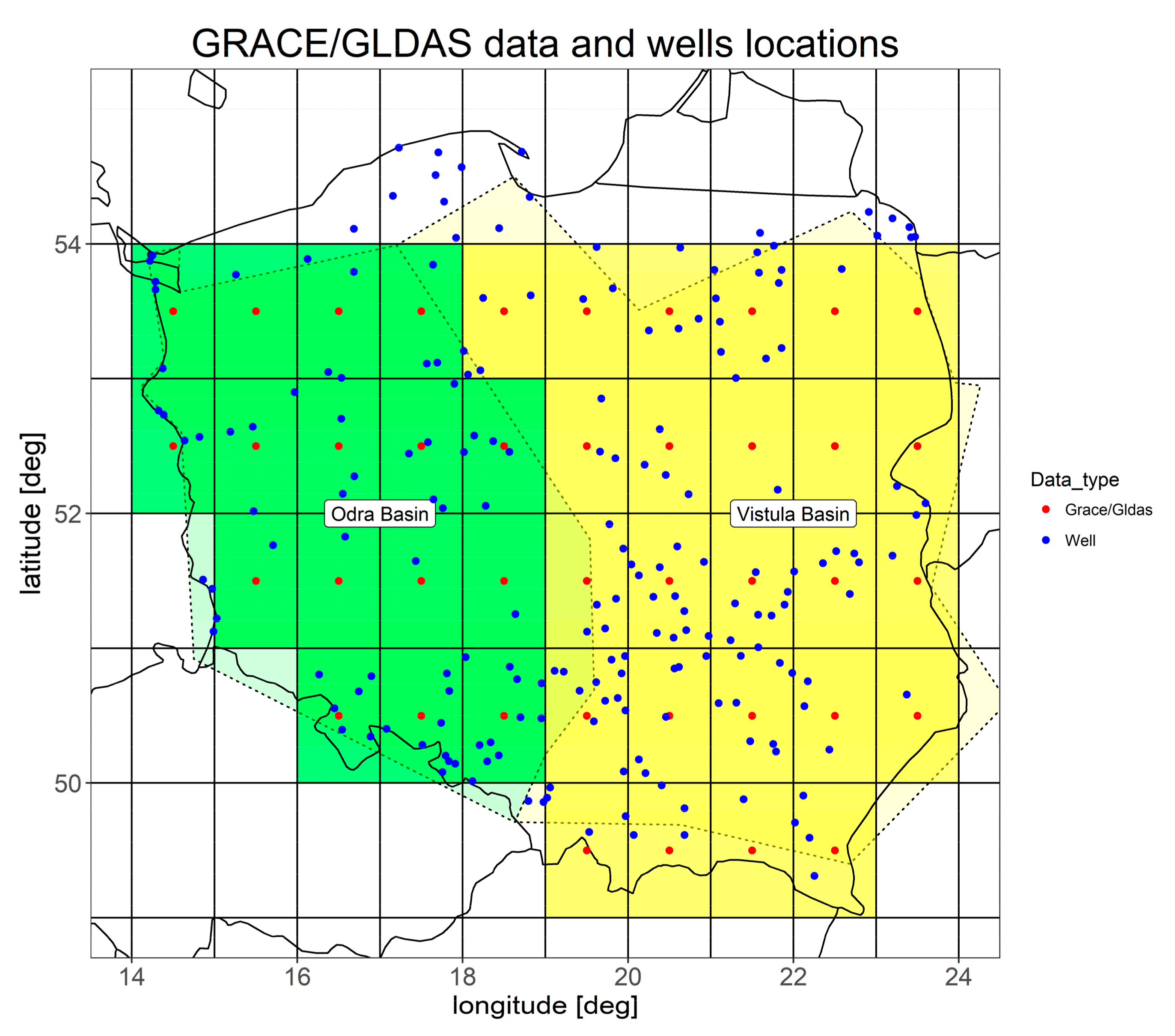
2.1. Study Area
2.2. Data Used
2.2.1. The GRACE Mission Data
2.2.2. GLDAS Models
2.2.3. CMIP5 Models
2.2.4. Groundwater Level from Wells
3. Methods
3.1. GWS from Groundwater Level Wells
3.2. TWS and GWS from GRACE and Models
3.3. Time Series Processing
4. Results
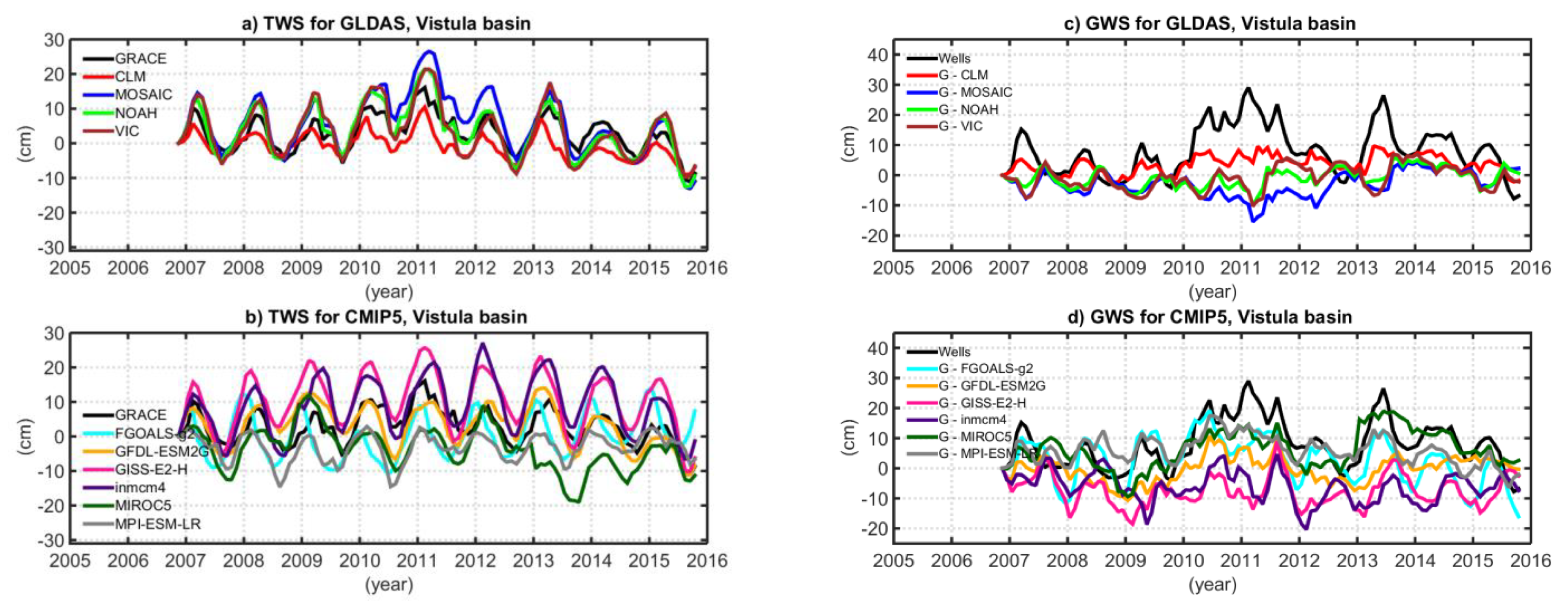
4.1. Time Series Comparison
4.2. Linear Trends of TWS and GWS
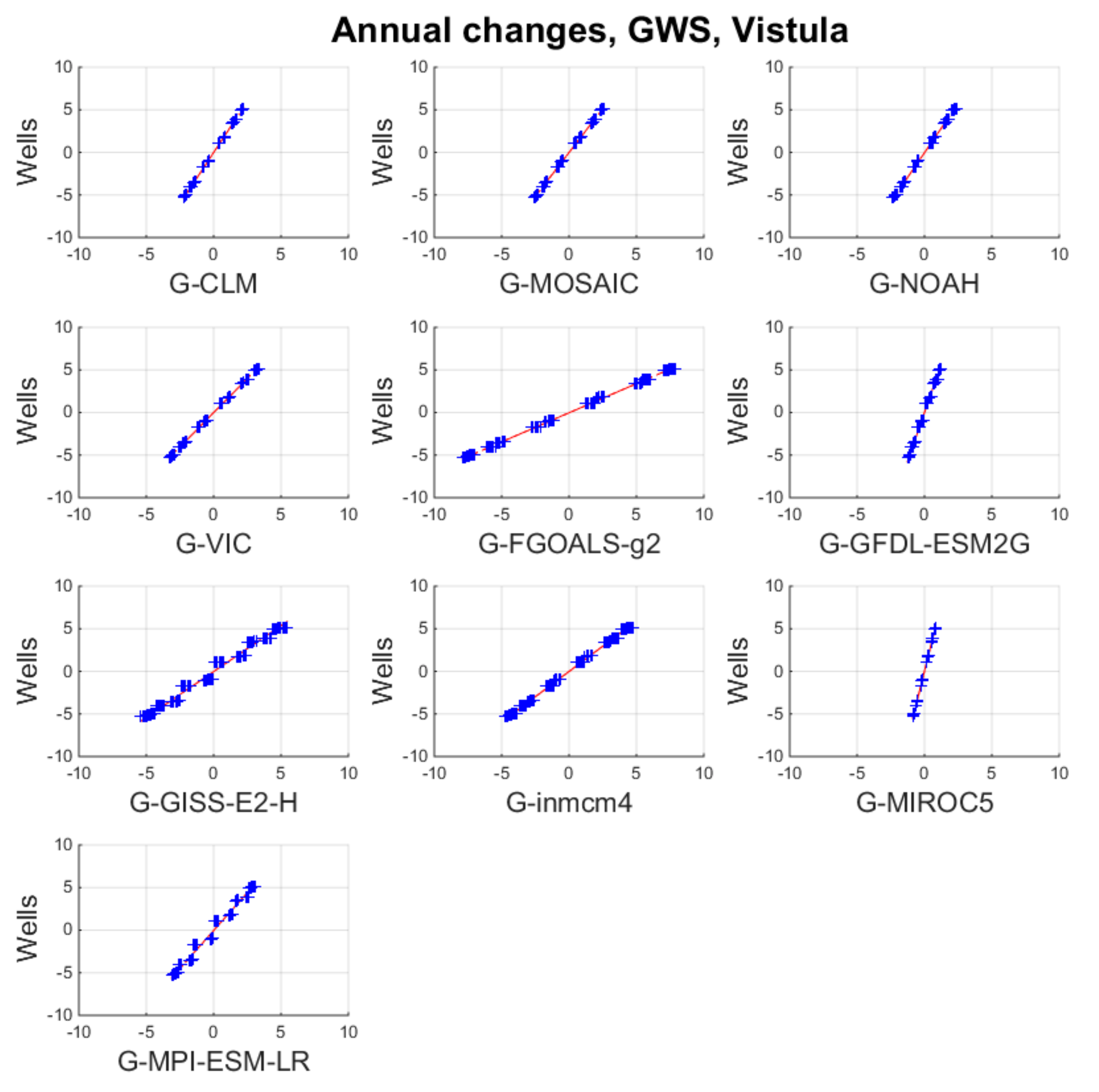
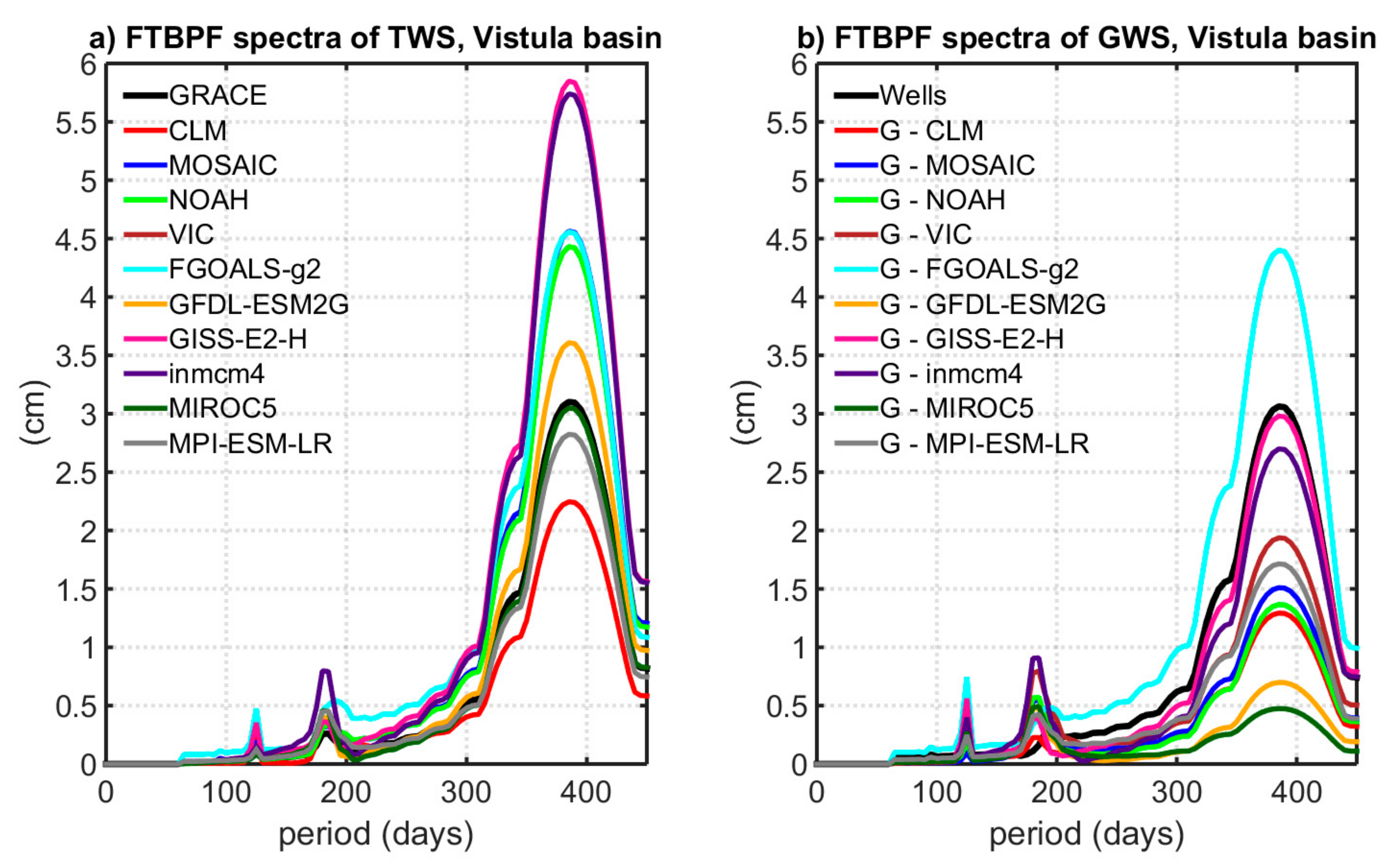
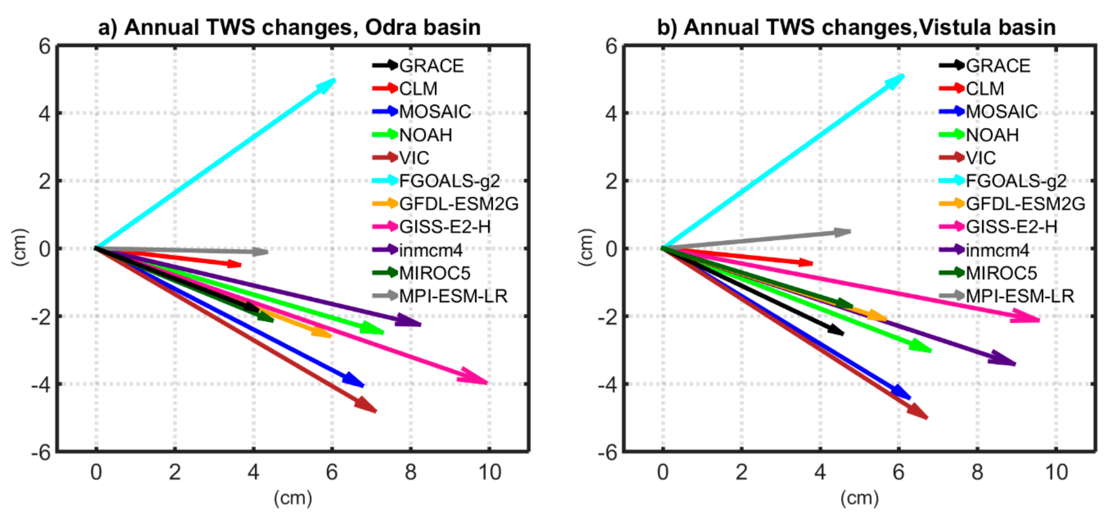
4.3. Seasonal Variations of TWS and GWS
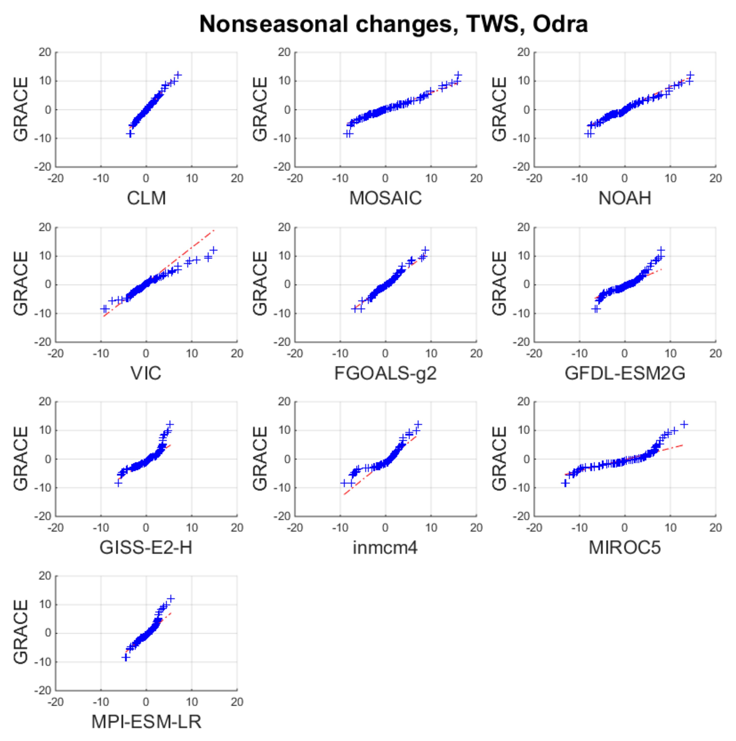
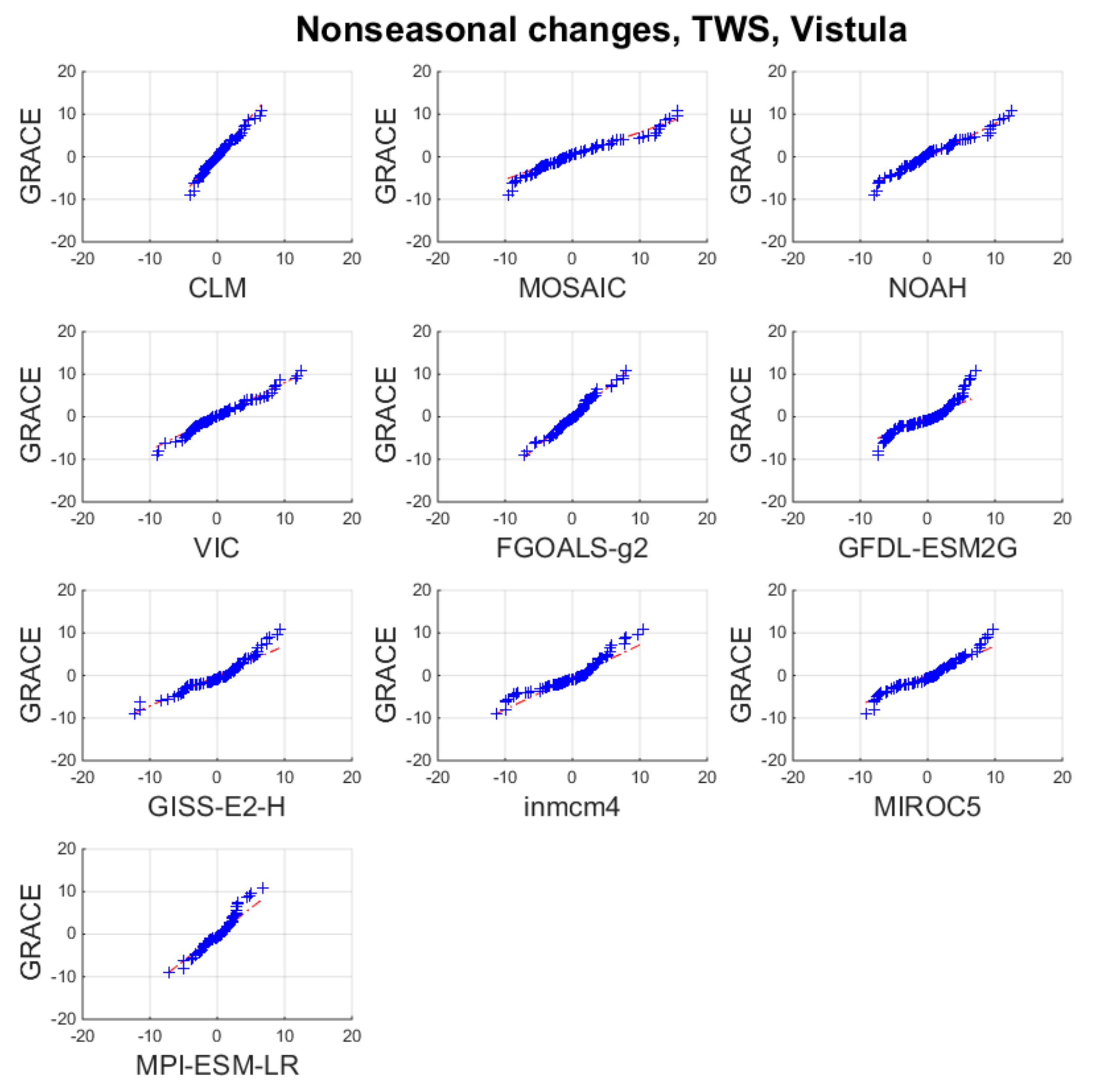
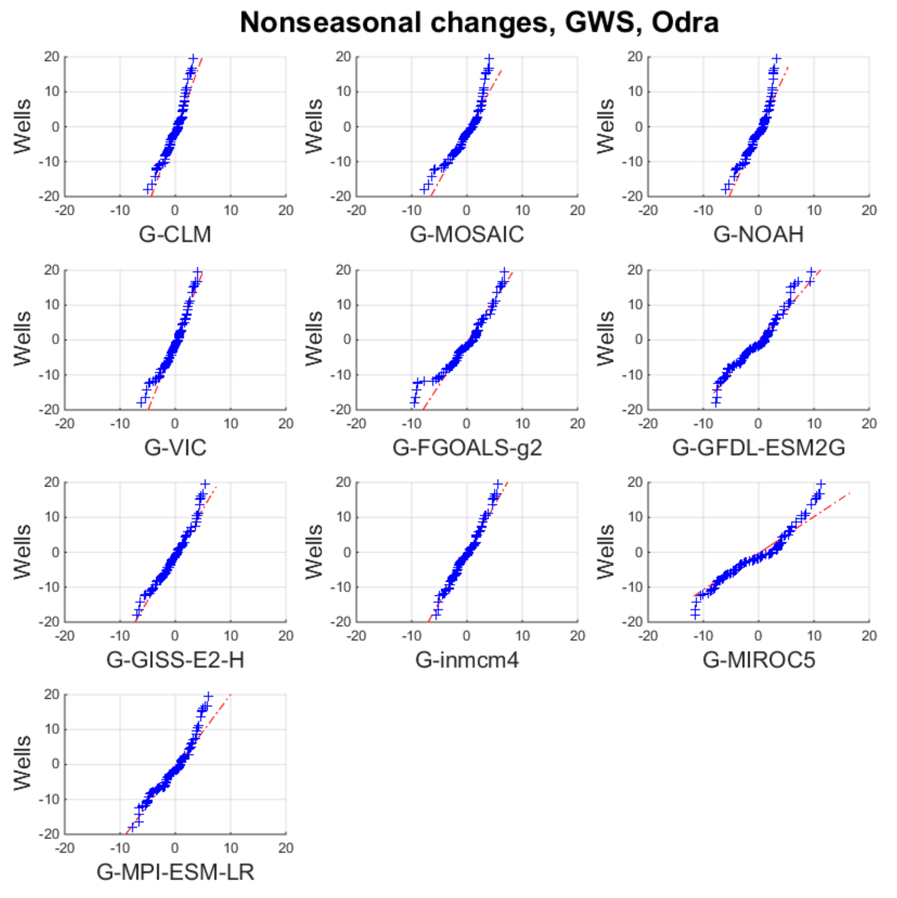
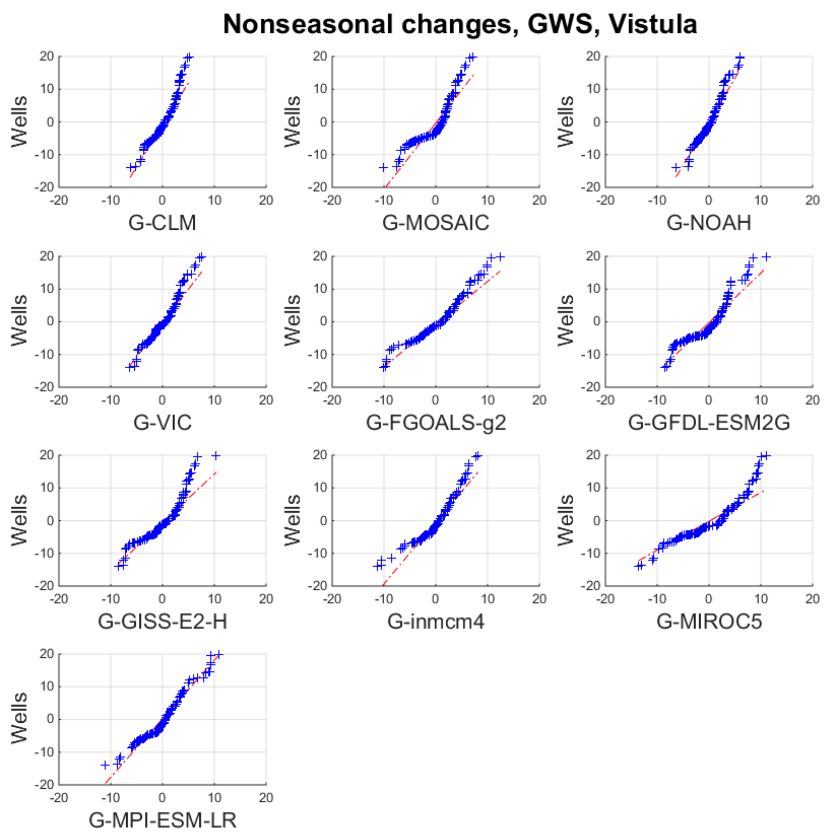
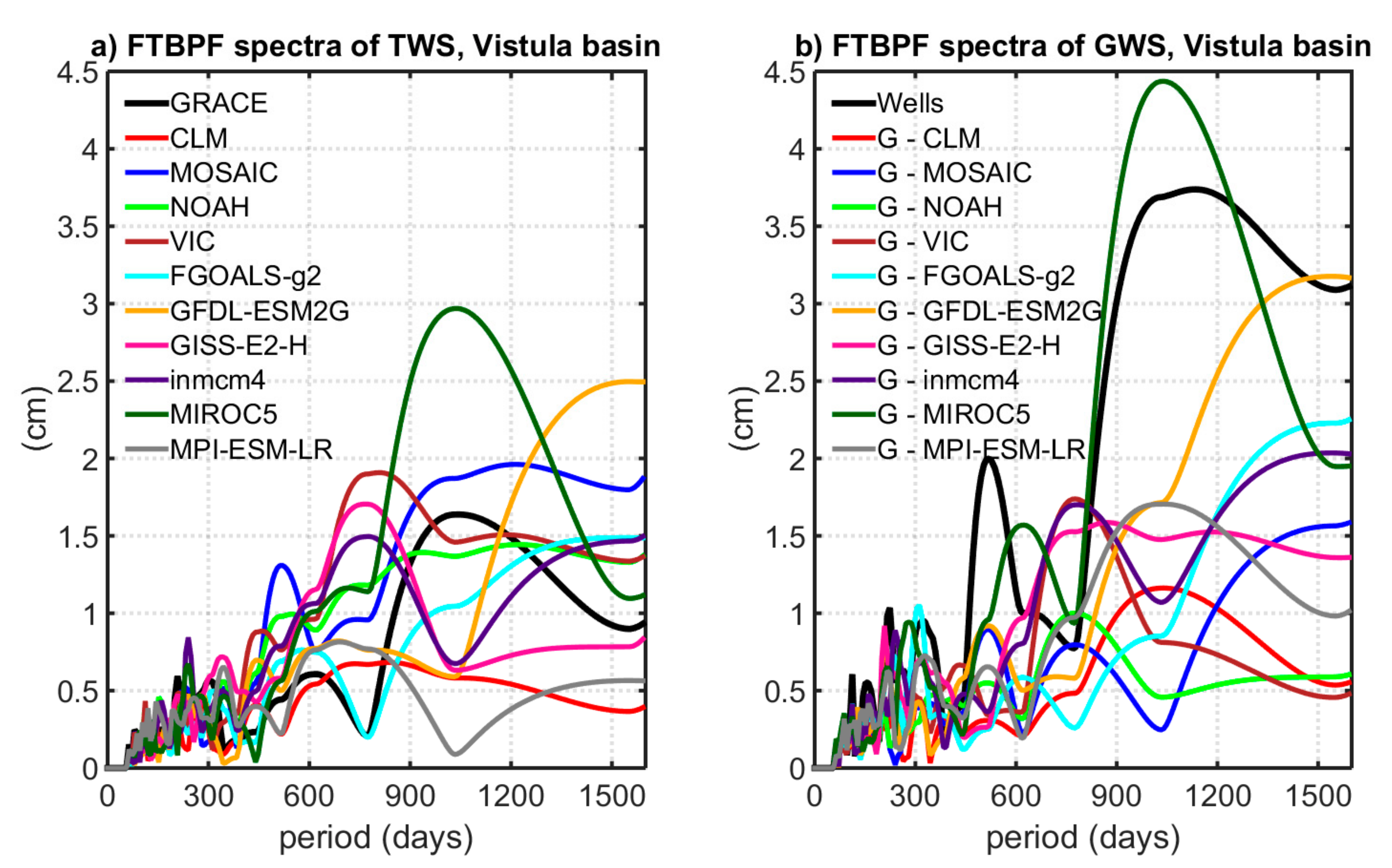
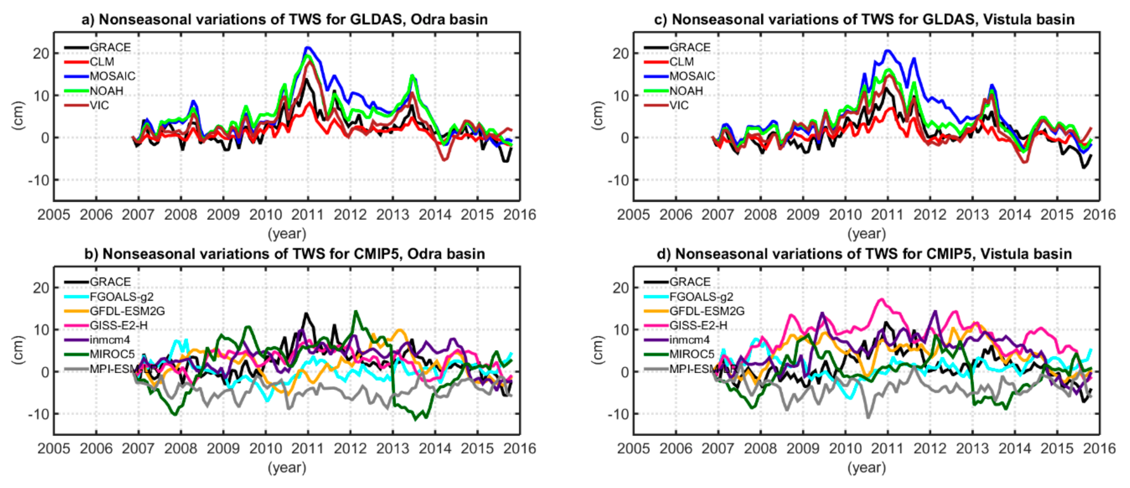
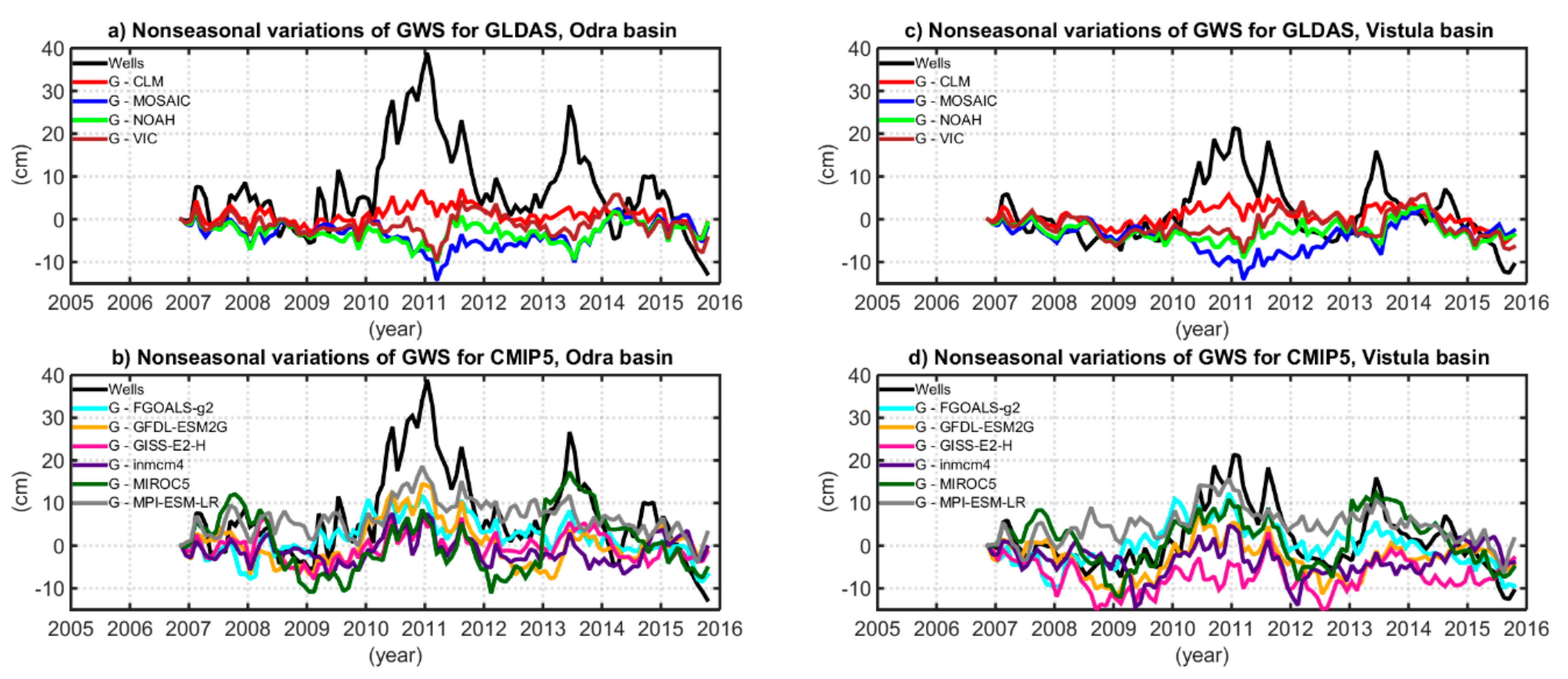
4.4. Non-seasonal Variations of TWS and GWS
5. Discussion
6. Summary and Conclusions
Author Contributions
Funding
Acknowledgments
Conflicts of Interest
Appendix

| TWS | Odra Basin | Vistula Basin | GWS | Odra Basin | Vistula Basin | ||||
|---|---|---|---|---|---|---|---|---|---|
| Error | R2 | Error | R2 | Error | R2 | Error | R2 | ||
| GRACE | 3.47 | 0.54 | 3.50 | 0.47 | Wells | 11.92 | 0.21 | 8.89 | 0.32 |
| CLM | 1.87 | 0.34 | 1.98 | 0.34 | GRACE–CLM | 2.08 | 0.80 | 2.33 | 0.67 |
| MOSAIC | 5.49 | 0.49 | 5.90 | 0.54 | GRACE–MOSAIC | 2.98 | 0.57 | 3.36 | 0.75 |
| NOAH | 4.58 | 0.41 | 4.37 | 0.41 | GRACE–NOAH | 2.31 | 0.48 | 2.30 | 0.63 |
| VIC | 4.07 | 0.31 | 4.25 | 0.34 | GRACE–VIC | 2.63 | 0.40 | 2.83 | 0.55 |
| FGOALS-g2 | 2.49 | 0.17 | 2.45 | 0.16 | GRACE–FGOALS-g2 | 4.26 | 0.42 | 4.76 | 0.43 |
| GFDL-ESM2G | 3.46 | 0.36 | 3.65 | 0.42 | GRACE–GFDL-ESM2G | 5.03 | 0.91 | 4.12 | 0.94 |
| GISS-E2-H | 2.48 | 0.10 | 4.10 | 0.26 | GRACE–GISS-E2-H | 3.22 | 0.34 | 3.68 | 0.51 |
| inmcm4 | 3.02 | 0.20 | 4.31 | 0.29 | GRACE–inmcm4 | 3.19 | 0.51 | 3.63 | 0.54 |
| MIROC5 | 6.27 | 0.76 | 4.29 | 0.59 | GRACE–MIROC5 | 6.87 | 0.98 | 5.88 | 0.98 |
| MPI-ESM-LR | 1.85 | 0.26 | 2.13 | 0.28 | GRACE–MPI-ESM-LR | 4.04 | 0.88 | 4.07 | 0.77 |


References
- Green, T.R.; Taniguchi, M.; Kooi, H.; Gurdak, J.J.; Allen, D.M.; Hiscock, K.M.; Treidel, H.; Aureli, A. Beneath the surface of global change: Impacts of climate change on groundwater. J. Hydrol. 2011, 405, 532–560. [Google Scholar] [CrossRef] [Green Version]
- Lambert, A.; Huang, J.; van der Kamp, G.; Henton, J.; Mazzotti, S.; James, T.S.; Courtier, N.; Barr, A.G. Measuring water accumulation rates using GRACE data in areas experiencing glacial isostatic adjustment: The Nelson River basin. Geophys. Res. Lett. 2013, 6118–6122. [Google Scholar] [CrossRef]
- Perez-Valdivia, C.; Sauchyn, D.; Vanstone, J. Groundwater levels and teleconnection patterns in the Canadian Prairies. Water Resour. Res. 2012, 48, W07516. [Google Scholar] [CrossRef]
- Watras, C.J.; Read, J.S.; Holman, K.D.; Liu, Z.; Song, Y.-Y.; Watras, A.J.; Morgan, S.; Stanley, E.H. Decadal oscillation of lakes and aquifers in the upper Great Lakes region of North America: Hydroclimatic implications. Geophys. Res. Lett. 2014, 41, 456–462. [Google Scholar] [CrossRef]
- Huang, J.; Pavlic, G.; Rivera, A.; Palombi, D.; Smerdon, B. Mapping groundwater storage variations with GRACE: A case study in Alberta, Canada. Hydrogeol. J. 2016, 24, 1663–1680. [Google Scholar] [CrossRef] [Green Version]
- Wada, Y.; van Beek, L.P.H.; van Kempen, C.M.; Reckman, J.W.T.M.; Vasak, S.; Bierkens, M.F.P. Global depletion of ground-water resources. Geophys. Res. Lett. 2010, 37, L20402. [Google Scholar] [CrossRef] [Green Version]
- Rodell, M.; Famiglietti, J.S. An analysis of terrestrial water storage variations in Illinois with implications for the Gravity Recovery and Climate Experiment (GRACE). Water Resour. Res. 2001, 37, 1327–1340. [Google Scholar] [CrossRef] [Green Version]
- Rodell, M.; Chen, J.; Kato, H.; Famiglietti, J.S.; Nigro, J.; Wilson, C.R. Estimating groundwater storage changes in the Mississippi River basin (USA) using GRACE. Hydrogeol. J. 2007, 15, 159–166. [Google Scholar] [CrossRef]
- Rodell, M.; Velicogna, I.; Famiglietti, J.S. Satellite-based estimates of groundwater depletion in India. Nature 2009, 460, 999–1002. [Google Scholar] [CrossRef] [Green Version]
- Rzepecka, Z.; Birylo, M.; Kuczynska-Siehien, J. Analysis of groundwater level variations and water balance in the area of the Sudety mountains. Acta Geodyn. Geomater. 2017, 14, 307–315. [Google Scholar] [CrossRef] [Green Version]
- Śliwińska, J.; Wińska, M.; Nastula, J. Terrestrial water storage variations and their effect on polar motion. Acta Geophys. 2019, 67, 17–39. [Google Scholar] [CrossRef] [Green Version]
- Freedman, F.R.; Pitts, K.L.; Bridger, A.F.C. Evaluation of CMIP climate model hydrological output for the Mississippi River Basin using GRACE satellite observations. J. Hydrol. 2014, 519, 3566–3577. [Google Scholar] [CrossRef]
- Güntner, A.; Stuck, J.; Werth, S.; Döll, P.; Verzano, K.; Merz, B. A global analysis of temporal and spatial variations in continental water storage. Water Resour. Res. 2007, 43, 1–19. [Google Scholar] [CrossRef]
- Frappart, F.; Papa, F.; Güntner, A.; Werth, S.; Santos da Silva, J.; Tomasella, J.; Seyler, F.; Prigent, C.; Rossow, W.B.; Calmant, S.; et al. Satellite-based estimates of groundwater storage variations in large drainage basins with extensive floodplains. Remote Sens. Environ. 2011, 115, 1588–1594. [Google Scholar] [CrossRef] [Green Version]
- Shamsudduha, M.; Taylor, R.G.; Longuevergne, L. Monitoring groundwater storage changes in the highly seasonal humid tropics: Validation of GRACE measurements in the Bengal Basin. Water Resour. Res. 2012, 48, 1–12. [Google Scholar] [CrossRef] [Green Version]
- Humphrey, V.; Gudmundsson, L.; Seneviratne, S.I. Assessing global water storage variability from GRACE: Trends, seasonal cycle, subseasonal anomalies and extremes. Surv. Geophys. 2016, 37, 357–395. [Google Scholar] [CrossRef] [Green Version]
- Long, D.; Pan, Y.; Zhou, J.; Chen, Y.; Hou, X.; Hong, Y.; Scanlon, B.R.; Longuevergne, L. Global analysis of spatiotemporal variability in merged total water storage changes using multiple GRACE products and global hydrological models. Remote Sens. Environ. 2017, 192, 198–216. [Google Scholar] [CrossRef]
- Scanlon, B.R.; Zhang, Z.; Save, H.; Sun, A.Y.; Müller Schmied, H.; van Beek, L.P.H.; Wiese, D.N.; Wada, Y.; Long, D.; Reedy, R.C.; et al. Global models underestimate large decadal declining and rising water storage trends relative to GRACE satellite data. Proc. Natl. Acad. Sci. USA 2018, 115, E1080–E1089. [Google Scholar] [CrossRef] [Green Version]
- Scanlon, B.R.; Zhang, Z.; Rateb, A.; Sun, A.; Wiese, D.; Save, H.; Beaudoing, H.; Lo, M.H.; Müller-Schmied, H.; Döll, P.; et al. Tracking Seasonal Fluctuations in Land Water Storage Using Global Models and GRACE Satellites. Geophys. Res. Lett. 2019, 46, 5254–5264. [Google Scholar] [CrossRef]
- Zhang, L.; Dobslaw, H.; Thomas, M. Globally gridded terrestrial water storage variations from GRACE satellite gravimetry for hydrometeorological applications. Geophys. J. Int. 2016. [Google Scholar] [CrossRef] [Green Version]
- Chen, C.; Kaban, M.K.; Thomas, M.; Güntner, A.; Du, J.; Wang, L. Increased water storage of Lake Qinghai during 2004–2012 from GRACE data, hydrological models, radar altimetry and in situ measurements. Geophys. J. Int. 2017, 212, 679–693. [Google Scholar] [CrossRef]
- Forootan, E.; Safari, A.; Mostafaie, A.; Schumacher, M.; Delavar, M.; Awange, J.L. Large-Scale Total Water Storage and Water Flux Changes over the Arid and Semiarid Parts of the Middle East from GRACE and Reanalysis Products. Surv. Geophys. 2017, 38, 591–615. [Google Scholar] [CrossRef] [Green Version]
- Hassan, A.; Jin, S. Water storage changes and balances in Africa observed by GRACE and hydrologic models. Geod. Geodyn. 2016. [Google Scholar] [CrossRef] [Green Version]
- Zhang, Z.; Chao, B.F.; Chen, J.; Wilson, C.R. Terrestrial water storage anomalies of Yangtze River Basin droughts observed by GRACE and connections with ENSO. Glob. Planet. Chang. 2015, 126, 35–45. [Google Scholar] [CrossRef]
- Chen, J.L.; Wilson, C.R.; Tapley, B.D.; Yang, Z.L.; Niu, G.Y. 2005 drought event in the Amazon River basin as measured by GRACE and estimated by climate models. J. Geophys. Res. Solid Earth 2009, 114. [Google Scholar] [CrossRef]
- Zhang, L.; Dobslaw, H.; Dahle, C.; Sasgen, I.; Thomas, M. Validation of MPI-ESM decadal hindcast experiments with terrestrial water storage variations as observed by the GRACE satellite mission. Meteorol. Z. 2015, 25, 685–694. [Google Scholar] [CrossRef]
- Zhang, L.; Dobslaw, H.; Stacke, T.; Güntner, A.; Dill, R.; Thomas, M. Validation of terrestrial water storage variations as simulated by different global numerical models with GRACE satellite observations. Hydrol. Earth Syst. Sci. 2017, 21, 821–837. [Google Scholar] [CrossRef] [Green Version]
- Mehan, S.; Gitau, M.W.; Flanagan, D.C. Reliable Future Climatic Projections for Sustainable Hydro-Meteorological Assessments in the Western Lake Erie Basin. Water 2019, 11, 581. [Google Scholar] [CrossRef] [Green Version]
- Chen, J.; Famigliett, J.S.; Scanlon, B.R.; Rodell, M. Groundwater Storage Changes: Present Status from GRACE Observations. Surv. Geophys. 2016, 37, 397–417. [Google Scholar] [CrossRef]
- Feng, W.; Shum, C.K.; Zhong, M.; Pan, Y. Groundwater storage changes in China from satellite gravity: An overview. Remote Sens. 2018, 10, 674. [Google Scholar] [CrossRef] [Green Version]
- Xiang, L.; Wang, H.; Steffen, H.; Wu, P.; Jia, L.; Jiang, L.; Shen, Q. Groundwater storage changes in the Tibetan Plateau and adjacent areas revealed from GRACE satellite gravity data. Earth Planet. Sci. Lett. 2016, 449, 228–239. [Google Scholar] [CrossRef] [Green Version]
- Huang, Z.; Yeh, P.J.F.; Pan, Y.; Jiao, J.J.; Gong, H.; Li, X.; Güntner, A.; Zhu, Y.; Zhang, C.; Zheng, L. Detection of large-scale groundwater storage variability over the karstic regions in Southwest China. J. Hydrol. 2019, 569, 409–422. [Google Scholar] [CrossRef]
- Voss, K.A.; Famiglietti, J.S.; Lo, M.; Linage, C.; Rodell, M.; Swenson, S.C. Groundwater depletion in the Middle East from GRACE with implications for transboundary water management in the Tigris-Euphrates-Western Iran region. Water Resour. Res. 2013, 49. [Google Scholar] [CrossRef] [PubMed] [Green Version]
- Chen, J.; Li, J.; Zhang, Z.; Ni, S. Long-term groundwater variations in Northwest India from satellite gravity measurements. Glob. Planet. Chang. 2014, 116, 130–138. [Google Scholar] [CrossRef] [Green Version]
- Zaki, N.A.; Haghighi, A.T.; Rossi, P.M.; Tourian, M.J.; Klove, B. Monitoring Groundwater Storage Depletion Using Gravity Recovery and Climate Experiment (GRACE) Data in Bakhtegan Catchment, Iran. Water 2019, 11, 1456. [Google Scholar] [CrossRef] [Green Version]
- Bhanja, S.N.; Mukherjee, A.; Saha, D.; Velicogna, I.; Famiglietti, J.S. Validation of GRACE based groundwater storage anomaly using in-situ groundwater level measurements in India. J. Hydrol. 2016, 543, 729–738. [Google Scholar] [CrossRef]
- Chinnasamy, P.; Maheshwari, B.; Prathapar, S. Understanding groundwater storage changes and recharge in Rajasthan, India through remote sensing. Water 2015, 7, 5547–5565. [Google Scholar] [CrossRef] [Green Version]
- Frappart, F.; Papa, F.; Güntner, A.; Tomasella, J.; Pfeffer, J.; Ramillien, G.; Emilio, T.; Schietti, J.; Seoane, L.; da Silva Carvalho, J.; et al. The spatio-temporal variability of groundwater storage in the Amazon River Basin. Adv. Water Resour. 2018, 124, 41–52. [Google Scholar] [CrossRef] [Green Version]
- Hu, K.; Awange, J.L.; Forootan, E.; Goncalves, R.M.; Fleming, K. Hydrogeological characterisation of groundwater over Brazil using remotely sensed and model products. Sci. Total Environ. 2017, 599–600, 372–386. [Google Scholar] [CrossRef] [Green Version]
- Scanlon, B.R.; Keese, K.E.; Flint, A.L.; Flint, L.E.; Gaye, C.B.; Edmunds, W.M.; Simmers, I. Global synthesis of groundwater recharge in semiarid and arid regions. Hydrol. Process. 2006, 20, 3335–3370. [Google Scholar] [CrossRef]
- Chen, J.L.; Wilson, C.R.; Tapley, B.D.; Scanlon, B.; Güntner, A. Long-term groundwater storage change in Victoria, Australia from satellite gravity and in situ observations. Glob. Planet. Chang. 2016, 139, 56–65. [Google Scholar] [CrossRef] [Green Version]
- Castle, S.L.; Thomas, B.F.; Reager, J.T.; Rodell, M.; Swenson, S.C.; Famiglietti, J.S. Groundwater depletion during drought threatens future water security of the Colorado River Basin. Geophys. Res. Lett. 2014, 41, 5904–5911. [Google Scholar] [CrossRef] [Green Version]
- Jin, S.; Feng, G. Large-scale variations of global groundwater from satellite gravimetry and hydrological models, 2002–2012. Glob. Planet. Chang. 2013, 106, 20–30. [Google Scholar] [CrossRef]
- Sadurski, A. Hydrogeological Annual Reports. In Polish Hydrological Survey. Hydrological Year 2015; Polish Geological Institute—National Research Institute: Warszawa, Poland, 2016. Available online: https://www.pgi.gov.pl/psh/materialy-informacyjne-psh/rocznik-hydrogeologiczny-psh.html (accessed on 1 June 2019).
- Rzepecka, Z.; Birylo, M.; Nastula, J. Assessment of Resultant Groundwater Calculated on the Basis of Grace and Gldas Models. In Proceedings of the 16th International Multidisciplinary Scientific Conference SGEM2016, Albena, Bulgaria, 30 June–6 July 2016; Book 2. Volume 2, pp. 125–132. [Google Scholar] [CrossRef]
- Rzepecka, Z.; Birylo, M.; Nastula, J. Evaluation of the Global Land Data Assimilation System (Gldas) Data Products Essential for Determination Groundwater in Poland. In Proceedings of the 16th International Multidisciplinary Scientific Conference SGEM2016, Albena, Bulgaria, 30 June–6 July 2016; Book 3. Volume 1, pp. 313–320. [Google Scholar] [CrossRef]
- Barlik, M.; Pachuta, A.; Olszak, T. Monitoring of long-term absolute gravity changes in Polish territory. In Proceedings of the XX Autumn School of Geodesy, Polanica, Poland, 16–18 September 2007; Available online: http://www.igig.up.wroc.pl/20jsg/prezentacje/Barlik_Szkola_Polanica_2007.pdf (accessed on 1 September 2019). (In Polish).
- Krynski, J.; Kloch-Glowka, G.; Szelachowska, M. Analysis of Time Variations of the Gravity Field Over Europe Obtained from GRACE Data in Terms of Geoid Height and Mass Variation. In Earth on the Edge: Science for a Sustainable Planet; Rizos, C., Willis, P., Eds.; International Association of Geodesy Symposia; Springer: Berlin/Heidelberg, Germany, 2014; Volume 139. [Google Scholar]
- Singh, A.K.; Jasrotia, A.S.; Taloor, A.K.; Kotlia, B.S.; Kumar, V.; Roy, S.; Ray, P.K.C.; Singh, K.K.; Singh, A.K.; Sharma, A.K. Estimation of quantitative measures of total water storage variation from GRACE and GLDAS-NOAH satellites using geospatial technology. Quat. Int. 2017, 444, 191–200. [Google Scholar] [CrossRef]
- Rzepecka, Z. Analysis of Terestrial Water Storage Variations on the Terrain of Vistula and Odra Basins in Poland. In Proceedings of the International Conference on Time Series and Forecasting, Grenada, Spain, 19–21 September 2018; Volume 3, ISBN 978-84-17293-57-4. [Google Scholar]
- Bonsor, H.C.; Shamsudduha, M.; Marchant, B.P.; MacDonald, A.M.; Taylor, R.G. Seasonal and decadal groundwater changes in African sedimentary aquifers estimated using GRACE products and LSMs. Remote Sens. 2018, 10, 904. [Google Scholar] [CrossRef] [Green Version]
- Iqbal, N.; Hossain, F.; Lee, H.; Akhter, G. Integrated groundwater resource management in Indus Basin using satellite gravimetry and physical modeling tools. Environ. Monit. Assess. 2017, 189, 1–16. [Google Scholar] [CrossRef]
- Jiang, Q.; Ferreira, V.G.; Chen, J. Monitoring groundwater changes in the Yangtze River basin using satellite and model data. Arab. J. Geosci. 2016, 9. [Google Scholar] [CrossRef]
- Zhao, K.; Li, X. Estimating terrestrial water storage changes in the Tarim River Basin using GRACE data. Geophys. J. Int. 2017, 211, 1449–1460. [Google Scholar] [CrossRef]
- Tapley, B.D.; Bettadpur, S.; Watkins, M.; Reigber, C. The gravity recovery and climate experiment: Mission overview and early results. Geophys. Res. Lett. 2004, 31, L09607. [Google Scholar] [CrossRef] [Green Version]
- Swenson, S.C. GRACE Monthly Land Water Mass Grids NETCDF RELEASE 5.0. Ver. 5.0; PO.DAAC: Pasadena, CA, USA; Available online: http://dx.doi.org/10.5067/TELND-NC005 (accessed on 1 September 2018).
- Swenson, S.; Yeh, P.J.F.; Wahr, J.; Famiglietti, J. A comparison of terrestrial water storage variations from GRACE with in situ measurements from Illinois. Geophys. Res. Lett. 2006, 33, 1–5. [Google Scholar] [CrossRef] [Green Version]
- Landerer, F.W.; Swenson, S.C. Accuracy of scaled GRACE terrestrial water storage estimates. Water Resour. Res. 2012. [Google Scholar] [CrossRef]
- Watkins, M.M.; Yuan, D. JPL Level-2 Processing Standards Document for Level-2 Product Release 05.1. Technical Report GRACE. pp. 327–744. Available online: http://podaac-ftp.jpl.nasa.gov/allData/grace/docs/L2-JPL_ProcStds_v5.1.pdf (accessed on 1 September 2019).
- Sakumura, C.; Bettadpur, S.; Bruinsma, S. Ensemble prediction and intercomparison analysis of GRACE time-variable gravity field models. Geophys. Res. Lett. 2014, 41, 1389–1397. [Google Scholar] [CrossRef]
- Rui, H.; Beaudoing, K.H. Readme Document for Global Land Data Assimilation System Version 2 (GLDAS-2) Products. Last Revised 15 November 2013. Available online: http://blog.sciencenet.cn/home.php?mod=attachmentid=54640 (accessed on 1 September 2019).
- Rodell, M.; Houser, P.R.; Jambor, U.; Gottschalck, J.; Mitchell, K.; Meng, C.-J.; Arsenault, K.; Cosgrove, B.; Radakovich, J.; Arsenault, K.; et al. The global land data assimilation system. Bull. Am. Meteorol. Soc. 2004, 85, 381–394. [Google Scholar] [CrossRef] [Green Version]
- Cao, Y.; Guo, H.; Liao, R.; Uradzinski, M. Analysis of water vapor characteristics of regional rainfall around Poyang Lake using ground-based GPS observations. Acta Geod. Geophys. 2016, 51, 467. [Google Scholar] [CrossRef] [Green Version]
- Birylo, M. Analyses of the time series based on atmospheric energy budget determination for the purpose of budget prognosis with ARMA method. In Proceedings of the ITISE 2018 International Conference on Time Series and Forecasting, Granada, Spain, 19–21 September 2018; Volume 3, ISBN 978-84-17293-57-4. [Google Scholar]
- Wang, W.; Cui, W.; Wang, X.; Chen, X. Evaluation of GLDAS-1 and GLDAS-2 Forcing Data and Noah Model Simulations over China at the Monthly Scale. J. Hydrometeorol. 2016, 17, 2815–2833. [Google Scholar] [CrossRef]
- Oleson, K.W.; Lawrence, D.M.; Bonan, G.B.; Flanner, M.G.; Kluzek, E.; Lawrence, P.J.; Levis, S.; Swenson, S.C.; Thornton, P.E. Technical Description of Version 4.0 of the Community Land Model (CLM), NCAR Tech. Note NCAR/TN-478+STR. pp. 1–257. Available online: https://opensky.ucar.edu/islandora/object/technotes%3A493/ (accessed on 1 September 2019).
- Rodell, M.; Beaudoing, K.H. GLDAS CLM Land Surface Model L4 Monthly 1.0 x 1.0 Degree V001, Greenbelt, Maryland, USA, Goddard Earth Sciences Data and Information Services Center (GES DISC). Available online: https://disc.gsfc.nasa.gov/datasets/GLDAS_CLM10_M_001/summary (accessed on 1 September 2019).
- Suarez, M.J.; Bloom, S.; Dee, D. Energy and Water Balance Calculations in the Mosaic LSM. NASA Tech Memo, 26. Available online: https://gmao.gsfc.nasa.gov/pubs/docs/Koster130.pdf (accessed on 1 September 2019).
- Rodell, M.; Beaudoing, K.H. GLDAS Mosaic Land Surface Model L4 Monthly 1.0 x 1.0 Degree V001, Greenbelt, Maryland, USA, Goddard Earth Sciences Data and Information Services Center (GES DISC). Available online: https://disc.gsfc.nasa.gov/datasets/GLDAS_MOS10_M_V001/summary (accessed on 1 September 2019).
- Rodell, M.; Beaudoing, K.H. GLDAS VIC Land Surface Model L4 Monthly 1.0 x 1.0 Degree V001, Greenbelt, Maryland, USA, Goddard Earth Sciences Data and Information Services Center (GES DISC. Available online: https://disc.gsfc.nasa.gov/datasets/GLDAS_VIC10_M_001/summary?keywords=gldas%20vic (accessed on 1 September 2019).
- Ek, M.B.; Mitchell, K.E.; Lin, Y.; Rogers, E.; Grunmann, P.; Koren, V.; Gayno, G.; Tarpley, J.D. Implementation of Noah land surface model advances in the National Centers for Environmental Prediction operational mesoscale Eta model. J. Geophys. Res. Atmos. 2003, 108, 8851. [Google Scholar] [CrossRef]
- Rodell, M.; Beaudoing, K.H. GLDAS Noah Land Surface Model L4 Monthly 1.0 x 1.0 Degree V001. Goddard Earth Sciences Data and Information Services Center (GES DISC): Greenbelt, MD, USA. Available online: https://disc.gsfc.nasa.gov/datasets/GLDAS_NOAH10_M_V001/summary (accessed on 1 September 2019).
- Rui, H.; Beaudoing, K.H. README Document for NASA GLDAS Version 2 Data Products, NASA’s Goddard Space Flight Center. Available online: http://hydro1.sci.gsfc.nasa.gov/data/s4pa/GLDAS/GLDAS_NOAH10_M.2.0/doc/README_GLDAS2.pdf (accessed on 1 September 2019).
- Taylor, K.E.; Stouffer, R.J.; Meehl, G.A. An overview of CMIP5 and the experiment design. Bull. Am. Meteorol. Soc. 2012, 93, 485–498. [Google Scholar] [CrossRef] [Green Version]
- Li, L.; Lin, P.; Yu, Y.; Wang, B.; Zhou, T.; Liu, L.; Liu, J.; Bao, Q.; Xu, S.; Huang, W.; et al. The Flexible Global Ocean-Atmosphere-Land System Model, Grid-point Version 2: FGOALS-g2. Adv. Atmos. Sci. 2013, 30, 543–560. [Google Scholar] [CrossRef]
- Dunne, J.P.; John, J.G.; Adcroft, A.J.; Griffies, S.M.; Hallberg, R.W.; Shevliakova, E.; Stouffer, R.J.; Cooke, W.; Dunne, K.A.; Harrison, M.J.; et al. GFDL’ s ESM2 Global Coupled Climate—Carbon Earth System Models. Part I: Physical Formulation and Baseline Simulation Characteristics. J. Clim. 2012, 25, 6646–6665. [Google Scholar] [CrossRef] [Green Version]
- Schmidt, G.A.; Kelley, M.; Nazarenko, L.S.; Ruedy, R.A.; Russell, G.L.; Aleinov, I.; Bauer, M.; Bauer, S.E.; Bhat, M.; Bleck, R.; et al. Configuration and assessment of the GISS Model E 2 contributions to the CMIP 5 archive. J. Adv. Model. Earth Syst. 2014, 6, 141–184. [Google Scholar] [CrossRef]
- Volodin, E.M.; Dianskii, N.A.; Gusev, A.V. Simulating Present Day Climate with the INMCM4.0 Coupled Model of the Atmospheric and Oceanic General Circulations. Atmos. Ocean. Phys. 2010, 46, 414–431. [Google Scholar] [CrossRef]
- Watanabe, M.; Suzuki, T.; O’ishi, R.; Komuro, Y.; Watanabe, S.; Emori, S.; Takemura, T.; Chikira, M.; Ogura, T.; Sekiguchi, M.; et al. Improved Climate Simulation by MIROC5: Mean States, Variability, and Climate Sensitivity. J. Clim. 2010, 23, 6312–6335. [Google Scholar] [CrossRef]
- Giorgetta, M.A.; Jungclaus, J.; Reick, C.H.; Legutke, S.; Bader, J.; Böttinger, M.; Brovkin, V.; Crueger, T.; Esch, M.; Fieg, K.; et al. Climate and carbon cycle changes from 1850 to 2100 in MPI-ESM simulations for the Coupled Model Intercomparison Project phase 5. J. Adv. Model. Earth Syst. 2013, 5, 572–597. [Google Scholar] [CrossRef]
- Sadurski, A. Hydrogeological Annual Reports. In Polish Hydrological Survey. Hydrological Year 2006; Polish Geological Institute—National Research Institute: Warsaw, Poland, 2007. [Google Scholar]
- Sadurski, A. Hydrogeological Annual Reports. In Polish Hydrological Survey. Hydrological Year 2007; Polish Geological Institute—National Research Institute: Warsaw, Poland, 2008. Available online: https://www.pgi.gov.pl/psh/materialy-informacyjne-psh/rocznik-hydrogeologiczny-psh.html (accessed on 1 June 2019).
- Sadurski, A. Hydrogeological Annual Reports. In Polish Hydrological Survey. Hydrological Year 2008; Polish Geological Institute—National Research Institute: Warsaw, Poland, 2009. Available online: https://www.pgi.gov.pl/psh/materialy-informacyjne-psh/rocznik-hydrogeologiczny-psh.html (accessed on 1 June 2019).
- Sadurski, A. Hydrogeological Annual Reports. In Polish Hydrological Survey. Hydrological Year 2009; Polish Geological Institute—National Research Institute: Warsaw, Poland, 2010. Available online: https://www.pgi.gov.pl/psh/materialy-informacyjne-psh/rocznik-hydrogeologiczny-psh.html (accessed on 1 June 2019).
- Sadurski, A. Hydrogeological Annual Reports. In Polish Hydrological Survey. Hydrological Year 2010; Polish Geological Institute—National Research Institute: Warsaw, Poland, 2011. Available online: https://www.pgi.gov.pl/psh/materialy-informacyjne-psh/rocznik-hydrogeologiczny-psh.html (accessed on 1 June 2019).
- Sadurski, A. Hydrogeological Annual Reports. In Polish Hydrological Survey. Hydrological Year 2011; Polish Geological Institute—National Research Institute: Warsaw, Poland, 2012. Available online: https://www.pgi.gov.pl/psh/materialy-informacyjne-psh/rocznik-hydrogeologiczny-psh.html (accessed on 1 June 2019).
- Sadurski, A. Hydrogeological Annual Reports. In Polish Hydrological Survey. Hydrological Year 2012; Polish Geological Institute—National Research Institute: Warsaw, Poland, 2013. Available online: https://www.pgi.gov.pl/psh/materialy-informacyjne-psh/rocznik-hydrogeologiczny-psh.html (accessed on 1 June 2019).
- Sadurski, A. Hydrogeological Annual Reports. In Polish Hydrological Survey. Hydrological Year 2013; Polish Geological Institute—National Research Institute: Warsaw, Poland, 2014. Available online: https://www.pgi.gov.pl/psh/materialy-informacyjne-psh/rocznik-hydrogeologiczny-psh.html (accessed on 1 June 2019).
- Sadurski, A. Hydrogeological Annual Reports. In Polish Hydrological Survey. Hydrological Year 2014; Polish Geological Institute—National Research Institute: Warsaw, Poland, 2015. Available online: https://www.pgi.gov.pl/psh/materialy-informacyjne-psh/rocznik-hydrogeologiczny-psh.html (accessed on 1 June 2019).
- Brewer, R.; Sleeman, J.R. Soil structure and fabric. Their definition and description. J. Soil Sci. 1960, 11, 172–185. [Google Scholar] [CrossRef]
- Konstankiewicz, K. Porowatość gleby, definicje i metody oznaczania (Soil porosity: Definitions and methods of determination). Probl. Agrofiz. 1985, 47. (In Polish) [Google Scholar]
- Rząsa, S.; Owczarzak, W. Porosity limits of polish soils. Zesz. Probl. Postępów Nauk Rol. 1992, 398, 139–144. [Google Scholar]
- Emerson, W.W.; McGarry, D. Organic carbon and soil porosity. Aust. J. Soil Res. 2003, 41, 107. Available online: https://trove.nla.gov.au/version/62565706 (accessed on 1 June 2019). [CrossRef] [Green Version]
- Eynard, A.; Schumacher, T.E.; Lindstrom, M.J.; Malo, D.D. Porosity and pore-size distribution in cultivated Ustolls and Usterts. Soil Sci. Soc. Am. J. 2004, 68, 1927–1934. [Google Scholar] [CrossRef]
- Głąb, T.; Kulig, B. Effect of mulch and tillage system on soil porosity under wheat (Triticum aestivum). Soil Tillage Res. 2008, 99, 169–178. [Google Scholar] [CrossRef]
- Kobierski, M.; Dąbkowska-Naskręt, H. Skład mineralogiczny i wybrane właściwości fizykochemiczne zróżnicowanych typologicznie gleb Równiny Inowrocławskiej. Cz. I. Morfologia oraz właściwości fizyczne i chemiczne wybranych gleb (Mineralogical composition and selected physicochemical properties of soils from Inowrocław Plain. Part, I. morphology and physical and chemical properties of selected soils). Rocz. Glebozn. Soil Sci. Annu. 2003, 54, 17–27. (In Polish) [Google Scholar]
- Paluszek, J. Water-air properties of eroded lessives soils developed from loess. Acta Agrophys. 2001, 56, 233–245. (In Polish) [Google Scholar]
- Paluszek, J. Quality of Structure and Water-Air Properties of Eroded Haplic Luvisol Treated with Gel-Forming Polymer. Pol. J. Environ. Stud. 2011, 19, 1287–1296. [Google Scholar]
- Xiao, R.; He, X.; Zhang, Y.; Ferreira, V.G.; Chang, L. Monitoring groundwater variations from satellite gravimetry and hydrological models: A comparison with in-situ measurements in the mid-atlantic region of the United States. Remote Sens. 2015, 7, 686–703. [Google Scholar] [CrossRef] [Green Version]
- Famiglietti, J.S.; Rodell, M. Water in the balance. Science 2013, 340, 1300–1301. [Google Scholar] [CrossRef] [PubMed]
- Rodell, M.; Famiglietti, J.S. The potential for satellite-based monitoring of groundwater storage changes using GRACE: The High Plains aquifer, Central US. J. Hydrol. 2002, 263, 245–256. [Google Scholar] [CrossRef] [Green Version]
- Sutanudjaja, E.H.; van Beek, L.P.H.; Drost, N.; de Graaf, I.E.M.; de Jong, K.; Peßenteiner, S.; Straatsma, M.W.; Wada, Y.; Wanders, N.; Wisser, D.; et al. PCR-GLOBWB 2.0: A 5 arc-minute global hydrological and water resources model. Geosci. Model Dev. 2018, 11, 2429–2453. [Google Scholar] [CrossRef] [Green Version]
- Yin, W.; Hu, L.; Jiao, J.J. Evaluation of Groundwater Storage Variations in Northern China Using GRACE Data. Geofluids 2017, 1–13. [Google Scholar] [CrossRef] [Green Version]
- Kosek, W. Time Variable Band Pass Filter Spectra of Real and Complex-Valued Polar Motion Series. Artif. Satell. 1995, 30, 27–43. [Google Scholar]
- Bissolli, P.; Friedrich, K.; Rapp, J.; Ziese, M. Flooding in eastern central Europe in May 2010—Reasons, evolution and climatological assessment. Weather 2011, 66, 147–153. [Google Scholar] [CrossRef]
- Argus, D.F.; Fu, Y.; Landerer, F.W. Seasonal variation in total water storage in California inferred from GPS observations of vertical land motion. Geophys. Res. Lett. 2014, 41, 1971–1980. [Google Scholar] [CrossRef]
- Barthelmes, F. Definition of Functionals of the Geopotential and their calculation from spherical harmonic models. Scientific Technical Report. (1). 1–5. Available online: http://gfzpublic.gfz-potsdam.de/pubman/item/escidoc:8786:4/component/escidoc:8785/0902.pdf (accessed on 1 September 2019).
- Swenson, S.C.; Wahr, J. Post-processing removal of correlated errors in GRACE data. Geophys. Res. Lett. 2006, 33, 1–4. [Google Scholar] [CrossRef]
- Watkins, M.M.; Wiese, D.N.; Yuan, D.-N.; Boening, C.; Landerer, F.W. Improved methods for observing Earth’s time variable mass distribution with GRACE using spherical cap mascons. J. Geophys. Res. Solid Earth 2015, 120, 2648–2671. [Google Scholar] [CrossRef]
- Rowlands, D.D.; Luthcke, S.B.; McCarthy, J.J.; Klosko, S.M.; Chinn, D.S.; Lemoine, F.G.; Boy, J.-P.; Sabaka, T.J. Global mass flux solutions from GRACE: A comparison of parameter estimation strategies—Mass concentrations versus Stokes coefficients. J. Geophys. Res. 2010, 115, B01403. [Google Scholar] [CrossRef]
- Eicker, A.; Schumacher, M.; Kusche, J.; Döll, P.; Schmied, H.M. Calibration/Data Assimilation Approach for Integrating GRACE Data into the WaterGAP Global Hydrology Model (WGHM) Using an Ensemble Kalman Filter: First Results. Surv. Geophys. 2014, 35, 1285–1309. [Google Scholar] [CrossRef]
- Khaki, M.; Forootan, E.; Kuhn, M.; Awange, J.; van Dijk, A.I.J.M.; Schumacher, M.; Sharifi, M.A. Determining water storage depletion within Iran by assimilating GRACE data into the W3RA hydrological model. Adv. Water Resour. 2018, 114, 1–18. [Google Scholar] [CrossRef] [Green Version]
- Kumar, S.V.; Zaitchik, B.F.; Peters-Lidard, C.D.; Rodell, M.; Reichle, R.; Li, B.; Jasinski, M.; Mocko, D.; Getirana, A.; De Lannoy, G.; et al. Assimilation of Gridded GRACE Terrestrial Water Storage Estimates in the North American Land Data Assimilation System. J. Hydrometeorol. 2016, 17, 1951–1972. [Google Scholar] [CrossRef]
- Reager, J.T.; Thomas, A.C.; Sproles, E.A.; Rodell, M.; Beaudoing, H.K.; Li, B.; Famiglietti, J.S. Assimilation of GRACE terrestrial water storage observations into a land surface model for the assessment of regional flood potential. Remote Sens. 2015, 7, 14663–14679. [Google Scholar] [CrossRef] [Green Version]
- Yin, W.; Hu, L.; Zhang, M.; Wang, J.; Han, S.C. Statistical Downscaling of GRACE-Derived Groundwater Storage Using ET Data in the North China Plain. J. Geophys. Res. Atmos. 2018, 123, 5973–5987. [Google Scholar] [CrossRef]
- Joseph, R.; Smith, T.M.; Sapiano, M.R.P.; Ferraro, R.R. A new high-resolution satellite-derived precipitation dataset for climate studies. J. Hydrometeorol. 2009, 10, 935–952. [Google Scholar] [CrossRef]
- Kummerow, C.; William, B.; Toshiaki, K.; James, S.; Simpson, J. The tropical rainfall measuring mission (TRMM) sensor package. Atmos. Ocean. Technol. 1998, 809, 15–17. [Google Scholar] [CrossRef]
- Marczewski, W.; Slominski, J.; Slominska, E.; Usowicz, B.; Usowicz, J.; Romanov, S.; Maryskevych, O.; Nastula, J.; Zawadzki, J. Strategies for validating and directions for employing SMOS data, in the Cal-Val project SWEX (3275) for wetlands. Hydrol. Earth Syst. Sci. Discuss. 2010, 7, 7007–7057. [Google Scholar] [CrossRef]


| Type of Data | Model/Data | Spatial Resolution | Comments | |
|---|---|---|---|---|
| Latitude (°) | Longitude (°) | |||
| GLDAS models | CLM | 1.000 | 1.000 | Monthly grids of TWS components (SM and SWE) |
| MOSAIC | 1.000 | 1.000 | ||
| NOAH | 1.000 | 1.000 | ||
| VIC | 1.000 | 1.000 | ||
| CMIP5 climate models | FGOALS-g2 | 3.000 | 2.812 | Monthly grids of TWS components (SM and SWE) |
| GFDL-ESM2G | 2.000 | 2.500 | ||
| GISS-E2-H | 2.000 | 2.500 | ||
| inmcm4 | 1.500 | 2.000 | ||
| MIROC5 | 1.406 | 1.406 | ||
| MPI-ESM-LR | 1.875 | 1.875 | ||
| GRACE | Mean of CSR RL05, JPL RL05, and GFZ RL05 solutions | 1.000 | 1.000 | Monthly grids of TWS anomalies relative to time-mean baseline |
| Ground Type | e |
|---|---|
| gravel | 0.30–0.40 |
| sands | 0.30–0.45 |
| loamy sands | 0.35–0.45 |
| sandy loams | 0.35–0.50 |
| sandy-clay loams | 0.40–0.55 |
| peat | 0.60–0.80 |
| silt | 0.54–1.00 |
| Soil Type | Vistula Basin | Odra Basin |
|---|---|---|
| Brown soils | 0.697 | 0.578 |
| Podzol soils | 0. 116 | 0.251 |
| Organic soils | 0.091 | 0.087 |
| Alluvial soils | 0.049 | 0.050 |
| Black earths | 0.033 | 0.025 |
| Rendzinas | 0.012 | 0.008 |
| Weighted mean | 0.41 | 0.42 |
| TWS | Odra Basin | Vistula Basin | ||||
|---|---|---|---|---|---|---|
| Trend | Trend Error | Coefficient of Determination (R2) | Trend | Trend Error | Coefficient of Determination (R2) | |
| GRACE | 0.00 | 0.26 | 0.99 | –0.21 | 0.29 | 0.97 |
| CLM | –0.49 | 0.18 | 0.82 | –0.56 | 0.19 | 0.80 |
| MOSAIC | –0.65 | 0.44 | 0.93 | –0.72 | 0.45 | 0.93 |
| NOAH | –0.58 | 0.40 | 0.93 | –0.67 | 0.38 | 0.91 |
| VIC | –0.52 | 0.41 | 0.94 | –0.68 | 0.41 | 0.92 |
| FGOALS-g2 | 0.82 | 0.34 | 0.92 | 0.70 | 0.34 | 0.95 |
| GFDL-ESM2G | –0.07 | 0.32 | 0.99 | –0.61 | 0.31 | 0.89 |
| GISS-E2-H | 0.06 | 0.45 | 0.99 | –0.03 | 0.45 | 0.99 |
| inmcm4 | 0.52 | 0.38 | 0.98 | 0.42 | 0.45 | 0.99 |
| MIROC5 | –2.50 | 0.40 | 0.53 | –1.03 | 0.31 | 0.78 |
| MPI-ESM-LR | 0.27 | 0.20 | 0.98 | 0.28 | 0.22 | 0.98 |
| GWS | Odra Basin | Vistula Basin | ||||
|---|---|---|---|---|---|---|
| Trend | Trend Error | Coefficient of Determination (R2) | Trend | Trend Error | Coefficient of Determination (R2) | |
| GRACE | 0.12 | 0.62 | 0.99 | 0.47 | 0.45 | 0.97 |
| CLM | 0.48 | 0.13 | 0.77 | 0.35 | 0.16 | 0.91 |
| MOSAIC | 0.64 | 0.22 | 0.82 | 0.50 | 0.22 | 0.88 |
| NOAH | 0.58 | 0.19 | 0.79 | 0.46 | 0.16 | 0.82 |
| VIC | 0.56 | 0.23 | 0.87 | 0.47 | 0.21 | 0.89 |
| FGOALS-g2 | –0.82 | 0.37 | 0.92 | –0.92 | 0.41 | 0.91 |
| GFDL-ESM2G | 0.06 | 0.30 | 0.99 | 0.40 | 0.24 | 0.93 |
| GISS-E2-H | –0.06 | 0.31 | 0.99 | –0.18 | 0.29 | 0.99 |
| inmcm4 | –0.52 | 0.25 | 0.94 | –0.64 | 0.28 | 0.92 |
| MIROC5 | 2.50 | 0.39 | 0.53 | 0.82 | 0.33 | 0.88 |
| MPI-ESM-LR | –0.28 | 0.24 | 0.97 | –0.50 | 0.26 | 0.93 |
| TWS | Correlation Coefficients | Relative Explained Variance (%) | RMSE (cm) | Month of Maximum | Phase (Days) | |||
|---|---|---|---|---|---|---|---|---|
| Full Time Series | Annual Changes | Full Time Series | Annual Changes | Full Time Series | Annual Changes | |||
| GRACE | − | − | − | − | − | − | March | 0.0 |
| CLM | 0.90 | 0.96 | 75.86 | 90.18 | 2.32 | 0.99 | February | 16.4 |
| MOSAIC | 0.92 | 0.99 | 30.52 | 39.33 | 3.93 | 2.46 | March | −7.1 |
| NOAH | 0.92 | 1.00 | 49.76 | 47.51 | 3.35 | 2.29 | March | 5.1 |
| VIC | 0.85 | 0.98 | 23.35 | 10.50 | 4.13 | 2.99 | March | −10.4 |
| FGOALS-g2 | 0.27 | 0.45 | −95.15 | −147.05 | 6.59 | 4.96 | January | 64.3 |
| GFDL-ESM2G | 0.51 | 1.00 | −24.87 | 80.16 | 5.27 | 1.41 | March | 0.3 |
| GISS-E2-H | 0.74 | 1.00 | −34.97 | −92.05 | 5.48 | 4.38 | March | 2.1 |
| inmcm4 | 0.75 | 0.99 | 9.44 | 14.25 | 4.49 | 2.93 | March | 8.6 |
| MIROC5 | 0.38 | 1.00 | −116.13 | 98.84 | 6.94 | 0.34 | March | −1.7 |
| MPI-ESM-LR | 0.49 | 0.92 | 17.09 | 85.25 | 4.30 | 1.21 | February | 22.7 |
| TWS | Correlation Coefficients | Relative Explained Variance (%) | RMSE (cm) | Month of Maximum | Phase (Days) | |||
|---|---|---|---|---|---|---|---|---|
| Full Time Series | Annual Changes | Full Time Series | Annual Changes | Full Time Series | Annual Changes | |||
| GRACE | − | − | − | − | − | − | March | 0.0 |
| CLM | 0.85 | 0.93 | 68.56 | 81.86 | 2.85 | 1.56 | February | 22.4 |
| MOSAIC | 0.92 | 0.99 | 41.85 | 75.89 | 3.88 | 1.80 | March | −6.4 |
| NOAH | 0.92 | 1.00 | 67.56 | 80.71 | 2.90 | 1.61 | March | 4.9 |
| VIC | 0.87 | 0.99 | 43.99 | 60.21 | 3.81 | 2.32 | March | −8.0 |
| FGOALS-g2 | 0.16 | 0.36 | −106.22 | −121.69 | 7.31 | 5.47 | January | 49.8 |
| GFDL-ESM2G | 0.69 | 0.99 | 30.27 | 94.97 | 4.25 | 0.82 | March | 8.6 |
| GISS-E2-H | 0.78 | 0.96 | −2.05 | 7.61 | 5.14 | 3.53 | February | 16.5 |
| inmcm4 | 0.81 | 0.99 | 6.06 | 26.19 | 4.93 | 3.15 | March | 8.0 |
| MIROC5 | 0.38 | 0.99 | −36.90 | 97.43 | 5.95 | 0.59 | March | 9.2 |
| MPI-ESM-LR | 0.50 | 0.82 | 17.04 | 66.39 | 4.63 | 2.13 | February | 35.4 |
| GWS | Correlation Coefficients | Relative Explained Variance (%) | RMSE (cm) | Month of Maximum | Phase (Days) | |||
|---|---|---|---|---|---|---|---|---|
| Full Time Series | Annual Changes | Full Time Series | Annual Changes | Full Time Series | Annual Changes | |||
| Wells− | − | − | − | − | − | − | April | 0.0 |
| GRACE–CLM | 0.74 | 0.96 | 26.69 | 36.35 | 9.46 | 3.70 | April | −17.0 |
| GRACE–MOSAIC | −0.67 | −0.97 | −60.24 | −131.26 | 13.99 | 7.04 | September | 196.9 |
| GRACE–NOAH | −0.55 | −0.74 | −42.29 | −97.77 | 13.18 | 6.51 | August | 225.2 |
| GRACE–VIC | −0.41 | −0.99 | −44.51 | −169.04 | 13.29 | 7.60 | October | 191.7 |
| GRACE–FGOALS-g2 | 0.61 | 0.62 | 37.56 | 17.71 | 8.73 | 4.20 | June | −52.5 |
| GRACE–GFDL-ESM2G | 0.55 | −0.86 | 29.25 | −61.18 | 9.30 | 5.88 | September | 214.1 |
| GRACE–GISS-E2-H | 0.06 | −0.83 | −19.13 | −246.72 | 12.06 | 8.62 | August | 216.7 |
| GRACE–inmcm4 | 0.17 | −0.67 | −2.33 | −124.60 | 11.18 | 6.94 | August | 231.1 |
| GRACE–MIROC5 | 0.37 | −0.97 | 6.42 | −14.80 | 10.69 | 4.96 | September | 194.3 |
| GRACE–MPI-ESM-LR | 0.72 | 0.73 | 40.52 | 31.15 | 8.52 | 3.84 | May | −43.4 |
| GWS | Correlation Coefficients | Relative Explained Variance | RMSE | Month of Maximum | Phase (Days) | |||
|---|---|---|---|---|---|---|---|---|
| Full Time Series | Annual Changes | Full Time Series | Annual Changes | Full time Series | Annual Changes | |||
| Wells− | − | − | − | − | − | − | April | 0.0 |
| GRACE–CLM | 0.80 | 1.00 | 44.25 | 66.14 | 5.96 | 2.17 | April | 1.5 |
| GRACE–MOSAIC | −0.64 | −0.92 | −85.88 | −112.38 | 10.89 | 5.44 | October | 205.4 |
| GRACE–NOAH | −0.31 | −0.53 | −35.62 | −64.68 | 9.30 | 4.79 | September | 241.2 |
| GRACE–VIC | −0.28 | −0.93 | −49.33 | −153.79 | 9.76 | 5.95 | October | 204.2 |
| GRACE–FGOALS-g2 | 0.70 | 0.86 | 44.98 | 37.69 | 5.92 | 2.95 | May | −31.1 |
| GRACE–GFDL-ESM2G | 0.57 | 0.03 | 32.85 | −3.42 | 6.55 | 3.80 | July | 276.0 |
| GRACE–GISS-E2-H | 0.17 | −0.26 | −20.11 | −138.34 | 8.75 | 5.77 | August | 258.5 |
| GRACE–inmcm4 | 0.06 | −0.52 | −30.51 | −158.57 | 9.12 | 6.01 | August | 242.3 |
| GRACE–MIROC5 | 0.66 | 0.82 | 42.42 | 23.25 | 6.06 | 3.27 | June | −34.4 |
| GRACE–MPI-ESM-LR | 0.76 | 0.92 | 54.81 | 37.67 | 5.37 | 1.95 | May | −22.7 |
| TWS | Correlation Coefficients | Relative Explained Variance (%) | RMSE (cm) | |||
|---|---|---|---|---|---|---|
| Odra | Vistula | Odra | Vistula | Odra | Vistula | |
| CLM | 0.86 | 0.77 | 55.56 | 64.19 | 2.08 | 2.33 |
| MOSAIC | 0.87 | 0.87 | 7.57 | 26.43 | 2.98 | 3.36 |
| NOAH | 0.87 | 0.85 | 56.86 | 55.67 | 2.33 | 2.31 |
| VIC | 0.77 | 0.75 | 34.43 | 42.56 | 2.64 | 2.83 |
| FGOALS-g2 | 0.00 | −0.26 | −85.64 | −50.87 | 4.29 | 4.78 |
| GFDL-ESM2G | −0.05 | 0.33 | −38.94 | −109.90 | 5.03 | 4.12 |
| GISS-E2-H | 0.46 | 0.54 | −11.02 | 14.00 | 3.28 | 3.73 |
| inmcm4 | 0.52 | 0.58 | −7.78 | 15.26 | 3.24 | 3.67 |
| MIROC5 | 0.09 | −0.13 | −183.34 | −292.39 | 6.87 | 5.89 |
| MPI-ESM-LR | −0.07 | 0.01 | −35.79 | −35.58 | 4.04 | 4.08 |
| GWS | Correlation Coefficients | Relative Explained Variance (%) | RMSE (cm) | |||
|---|---|---|---|---|---|---|
| Odra | Vistula | Odra | Vistula | Odra | Vistula | |
| GRACE–CLM | 0.70 | 0.75 | 24.71 | 38.51 | 8.69 | 5.53 |
| GRACE–MOSAIC | −0.59 | −0.57 | −43.98 | −77.13 | 12.02 | 9.38 |
| GRACE–NOAH | −0.51 | −0.23 | −29.08 | −25.78 | 11.38 | 7.91 |
| GRACE–VIC | −0.17 | −0.01 | −15.98 | −17.17 | 10.79 | 7.63 |
| GRACE–FGOALS-g2 | 0.70 | 0.69 | 41.75 | 47.37 | 7.67 | 5.13 |
| GRACE–GFDL-ESM2G | 0.74 | 0.67 | 49.15 | 43.71 | 7.15 | 5.29 |
| GRACE–GISS-E2-H | 0.62 | 0.39 | 29.58 | 13.29 | 8.45 | 6.59 |
| GRACE–inmcm4 | 0.55 | 0.33 | 25.23 | 7.53 | 8.69 | 6.80 |
| GRACE–MIROC5 | 0.43 | 0.71 | 11.52 | 48.46 | 9.42 | 5.06 |
| GRACE–MPI-ESM-LR | 0.73 | 0.72 | 42.86 | 50.07 | 7.57 | 4.98 |
© 2019 by the authors. Licensee MDPI, Basel, Switzerland. This article is an open access article distributed under the terms and conditions of the Creative Commons Attribution (CC BY) license (http://creativecommons.org/licenses/by/4.0/).
Share and Cite
Śliwińska, J.; Birylo, M.; Rzepecka, Z.; Nastula, J. Analysis of Groundwater and Total Water Storage Changes in Poland Using GRACE Observations, In-situ Data, and Various Assimilation and Climate Models. Remote Sens. 2019, 11, 2949. https://doi.org/10.3390/rs11242949
Śliwińska J, Birylo M, Rzepecka Z, Nastula J. Analysis of Groundwater and Total Water Storage Changes in Poland Using GRACE Observations, In-situ Data, and Various Assimilation and Climate Models. Remote Sensing. 2019; 11(24):2949. https://doi.org/10.3390/rs11242949
Chicago/Turabian StyleŚliwińska, Justyna, Monika Birylo, Zofia Rzepecka, and Jolanta Nastula. 2019. "Analysis of Groundwater and Total Water Storage Changes in Poland Using GRACE Observations, In-situ Data, and Various Assimilation and Climate Models" Remote Sensing 11, no. 24: 2949. https://doi.org/10.3390/rs11242949