Multi-Scale Relationship between Land Surface Temperature and Landscape Pattern Based on Wavelet Coherence: The Case of Metropolitan Beijing, China

Abstract

The relationship between urban landscape pattern and land surface temperature (LST) is one of the core issues in urban thermal environment research. Although previous studies have shown a significant correlation between LST and landscape pattern, most were conducted at a single scale and rarely involve multi-scale effects of the landscape pattern. Wavelet coherence can relate the correlation between LST and landscape pattern to spatial scale and location, which is an effective multi-scale correlation method. In this paper, we applied wavelet coherence and Pearson correlation coefficient to analyze the multi-scale correlations between landscape pattern and LST, and analyzed the spatial pattern of the urban thermal environment during the urbanization of Beijing from 2004 to 2017 by distribution index of high-temperature center (HTC). The results indicated that the HTC of Beijing gradually expands from the main urban zone and urban function extended zone to the new urban development zone and far suburb zone, and develops from monocentric to polycentric spatial pattern. Land cover types, such as impervious surfaces and bare land, have a positive contribution to LST, while water and vegetation play a role in mitigating LST. The wavelet coherence and Pearson correlation coefficients showed that landscape composition and spatial configuration have significant effects on LST, but landscape composition has a greater effect on LST in Beijing metropolitan area. Landscape composition indexes (NDBI and NDVI) showed significant multi-scale characteristics with LST, especially at larger scales, which has a strong correlation on the whole transect. There was no significant correlation between the spatial configuration indexes (CONTAG, DIVISION, and LSI) and LST at smaller scales, only at larger scales near the urban area has a significant correlation. With the increase of the scale, Pearson correlation coefficient calculated by spatial rectangle sampling and wavelet coherence coefficient have the same trend, although it had some fluctuations in several locations. However, the wavelet coherence coefficient diagram was smoother and less affected by position and rectangle size, which more conducive to describe the correlation between landscape pattern index and LST at different scales and locations. In general, wavelet coherence provides a multi-scale method to analyze the relationship between landscape pattern and LST, helping to understand urban planning and land management to mitigate the factors affecting urban thermal environment.

1. Introduction

Rapid urbanization has tremendously changed the urban landscape pattern, which is one of the most remarkable human land surface activities since the 20th century [1,2,3]. As the process of transforming natural landscapes (such as water, vegetation, and cultivated land) into artificial impervious surfaces, urbanization has a profound impact on urban ecosystems, including biodiversity, energy flows, biogeochemical cycles, local regional climates, and human health [4,5,6,7]. Land surface temperature (LST) is one of the direct manifestations of urban thermal environment impacted by land cover or land use types and landscape pattern [8,9]. The spatial distribution of LST, especially excessive concentration of high-temperature centers (HTC), may bring a lot of disadvantages to the health of urban residents and the living environment of animal and vegetable life [10]. Identification of the spatial pattern dynamics of urban temperature and the relationship between landscape pattern and LST are important for urban planning and management [11,12].

Landscape pattern has two fundamental aspects: landscape composition and spatial configuration, and significantly affect the urban LST [10,13,14]. Landscape composition refers to the richness and diversity of patches, usually described by different types of land cover and their proportion [15,16]. Landscape configuration focuses on describing the spatial combination and morphology of landscape patches [9,15]. Previous studies have focused on the effects of landscape composition (mainly land cover types) on LST, and different land cover types have unique radiation and specific heat capacity with various effects on LST [17,18]. Impervious surface and bare land have a relative highly radiation and lower specific heat capacity, which are generally considered to increase urban LST, while the low radiation and transpiration of water and vegetation with the appositive radiative characteristics can mitigate urban LST [19,20]. With the acceleration of urbanization, the changes of urban land cover types have intensified, and the effects of landscape space configuration on LST has received increasing attention, especially the identification of relationship between the fragmentation, aggregation, and spatial morphology of landscape patches and LST [13,21,22,23].

The major models to quantify the relationship between landscape pattern and LST include correlation coefficient, regression analysis, principal component regression analysis, and spatial analysis [10,24,25]. Most of these models analyzed the effects of landscape pattern metrics on LST at a single scale, and the hierarchical structure and scale dependence of landscape patterns were usually ignored [26,27]. In order to solve these issues, researchers have selected some analysis scales and calculated the correlation between LST and landscape metrics at the corresponding scales to reveal their multi-scale characteristics [10,11,28,29]. However, the scale of artificial selection is usually subjective, with the disadvantages to ensure accuracy and fineness, and may cause the correlation loss between adjacent scales. Wavelet analysis is a multi-scale analysis method, which can associate landscape pattern with scale and location, and has shown better scale continuity [30,31,32]. Wavelet coherent analysis examines the multi-scale correlated characteristics within time-frequency localization, and has the advantages to solve complex ecological correlations among large number of ecological indices [33,34,35]. Grinsted et al. analyzed the relationship between the Baltic maximum sea ice extent and the Arctic Oscillation index used wavelet coherence, revealed the multi-scale correlation and periodicity [33]. Biswas applied wavelet coherence to study the multi-scale correlation between soil depths and spatial patterns of soil water storage, demonstrating that wavelet coherence can be used to determine the correlation between different ecological factors at a given scales and location [36]. Landscape pattern has scale dependence, and multi-scale effects need to be considered when studying its effects on LST [10]. Therefore, wavelet coherence may be an effective method to identify the multi-scale correlation between LST and landscape pattern [35,36,37]. Additionally, this paper may be the first work to date that deals with multi-scale correlation analysis between landscape patterns and LST using wavelet coherence.

Beijing has experienced rapid urbanization since the 1980s, and the built-up area has increased from 490 km² (2004) to 1401 km² (2016), and population increased from 14.92 million to 21.73 million [38,39]. In order to provide more habitats, the green space and rural cultivated land around the urban area were tremendously occupied, and land cover types and spatial pattern have undergone tremendous changes, which have seriously affected the urban thermal environment [9,10]. The purpose of this study is to quantify the multi-scale relationship between LST and landscape pattern in Beijing metropolitan areas. Specifically, the study aims were to (1) quantify the dynamic of LST spatial pattern in Beijing from 2004 to 2017 by distribution index; (2) identify the multi-scale correlation between landscape pattern (landscape composition and spatial configuration index) and LST using wavelet coherence; (3) calculate the Pearson correlation coefficient between landscape indexes and LST by spatial rectangle sampling method and compared with wavelet coherence; (4) summarize the performance of wavelet coherence for the multi-scale correlation analysis of landscape pattern and the factors affected by them.

2. Materials and Methods

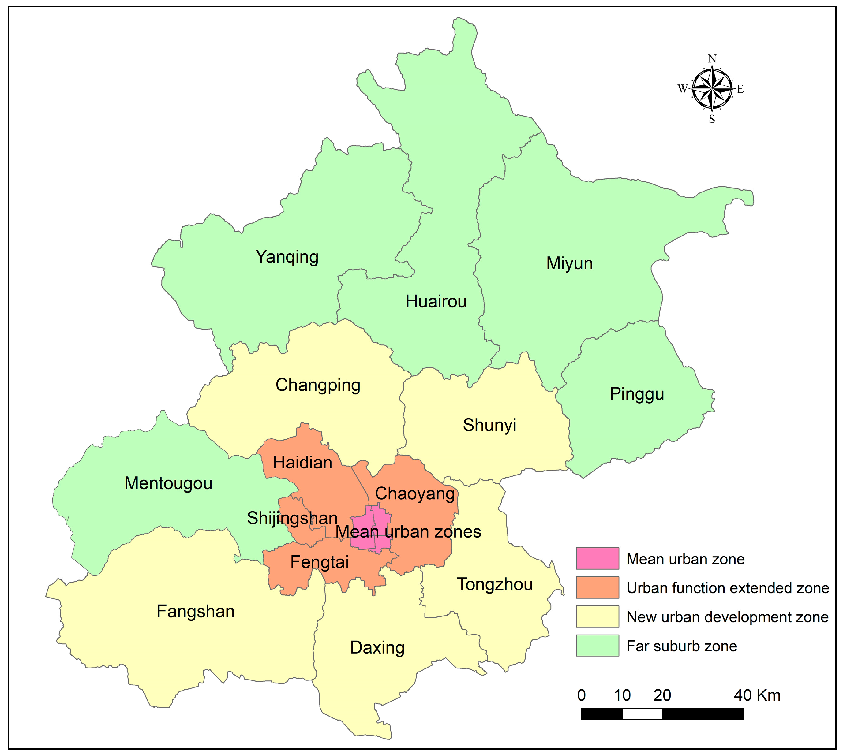
2.1. Study Area

Beijing is situated at 115.7°–117.4° E and 39.4°–41.6° N, with an area of 16,410.54 km². It includes 16 administrative areas, the northern and western regions are mainly mountainous areas, and the urban area is distributed in the southern plain area [38,39,40]. According to Beijing’s urban master plan (2004–2020), Beijing can be divided into four functional zones (Figure 1): the main urban zone (MUZ), urban function extended zone (UFEZ), new urban development zone (NUDZ), and far suburb zone (FSZ). The main urban zone includes Dongcheng, Xicheng, Xuanwu, and Chongwen (after 2010, Xuanwu District was merged into Xicheng District and Chongwen District was merged into Dongcheng District); the urban function extended zone includes Haidian, Chaoyang, Shijingshan, and Fengtai; the new urban development zone includes Fangshan, Daxing, Tongzhou, Shunyi, and Changping; the far suburb zone includes Yanqing, Huairou, Miyun, Pinggu, and Mentougou.

2.2. Data and Preprocessing

Two remote sensing images obtained in late summer (September) with highly clear atmospheric conditions (cloud amount less than 5%) were used in this study (

Table 1. The experimental data collected in this study.

Sensor	Scene ID	Acquisition Data	Season
Landsat-5 TM	LT51230322004252BJC00	8 September 2004	Summer
Landste-8 OLI/TIRS	LC81230322017255LGN00	12 September 2017	Summer

), and both the two remote sensing images were downloaded from the official website of USGS (https://earthexplorer.usgs.gov/). The two Landsat data sets in 2004 and 2017 are basically in accordance with the start year of Beijing Master Plan (2004–2020) and the start year of Beijing Master Plan (2016–2035) released by the government with detailed land-use types, which are very helpful for the validation of the land use classification from the two Landsat data sets. The climate of Beijing has the characteristics of the semi-humid continental monsoon climate in the north temperature zone. The weather is cold and dry in winter, with short duration in spring and autumn. Peng et al. studied the spatial pattern of Beijing’s urban thermal environment, and testified that urban heat island effects of summertime are more significant than that of other seasons, which can be considered as the reasonable season to study the urban thermal environment [9].

The land surface temperature was retrieved based on the single window algorithm after preprocessing including geometric correction, radiation correction, and atmospheric correction. Land cover maps were obtained by supervised classification and visual interpretation with a resolution of 30 m (Figure 2), which were classified into six classed including impervious surface (built-up land, roads, parking lots and other artificial impervious areas), urban green space (urban grass and park), water (rivers, lakes, and reservoirs), forest land (forest and shrubs), cultivated land and bare land (cradled and sand land). In order to improve the classification quality and solve misclassification error or salt-and-pepper noises generated by spectral confusion, Sieve Classes of ENVI was applied to remove the isolated points (the parameters were set as minimum threshold 2 pixels, window size 8 pixels), and visual interpretation of the classified maps and manual correction was conducted according to the existing two periods land use data (2004 and 2017) of Beijing Master Plan (2004–2020). To verify the classification accuracy, 34,596 points was randomly selected based on the proportion of each land, and the existing two periods land use data (2004 and 2017) of Beijing Master Plan (2004–2020) and historical images of Google Earth were referenced to make judgments and statistics on the classification accuracy of the sample points. The classification confusion matrix calculated from the samples and the classification accuracy of each land cover type are shown in

Table 2. The classification confusion matrix and accuracy.

Types	Bare Land	Water	Urban Green Space	Cultivated Land	Forest Land	Impervious Surface	User’s Accuracy
2004
Bare land	285	0	0	7	47	8	82.13%
Water	0	719	7	16	117	23	81.53%
Urban green space	0	8	563	23	86	17	80.77%
Cultivated land	19	9	13	7513	1836	49	79.60%
Forest land	30	76	43	1525	16,077	580	87.70%
Impervious surface	9	15	6	76	947	3847	78.51%
Producer’s accuracy	83.09%	86.94%	89.08%	82.02%	84.13%	85.04%
OA: 83.84% Kappa coefficient: 0.737
2017
Bare land	535	0	5	6	83	16	82.95%
Water	0	590	9	10	96	24	80.93%
Urban green space	0	3	747	37	117	13	81.46%
Cultivated land	56	55	15	5193	963	69	81.77%
Forest land	34	31	43	668	14,452	1144	88.27%
Impervious surface	23	24	17	192	1483	7843	81.85%
Producer’s accuracy	82.56%	83.93%	89.35%	85.05%	84.05%	86.10%
OA: 84.87% Kappa coefficient: 0.770

, where the overall accuracy (OA) of the land cover maps were 83.84% (2004) and 84.87% (2017), and the kappa coefficients were 0.737 (2004) and 0.770 (2017), respectively.

2.3. Land Surface Temperature Retrieval

The LST was retrieved from thermal infrared band of remote sensing images based on the single window algorithm [9,35]. The steps are as follows: (1) converting the digital number values of the thermal infrared band to surface-leaving radiance; (2) converting the surface-leaving radiance to at-sensor brightness temperature; (3) converting the at-sensor brightness temperature to LST [41,42].

First, the digital number (DN) of the thermal infrared band was converted to sensor radiance values (L_λ) using Equation (1) [43].

$$L_{\lambda }=\frac{LMA{X}_{\lambda }-LMI{N}_{\mu }}{Q_{calmax}-Q_{calmin}}\times \left(Q_{cal}-Q_{calmin}\right),$$

(1)

where $Q_{calmin}$ is the minimum quantized calibration digital number, $Q_{calmax}$ is the maximum quantized calibration digital number, $LMI{N}_{\mu }$ and $LMA{X}_{\lambda }$ are the ratios of spectral irradiance to $Q_{calmin}$ and $Q_{calmax}$, respectively.

Then the sensor radiance values can be converted to surface-leaving radiance through an atmospheric correction process using Equation (2).

$$L_T=\frac{L_{\lambda }-L_{\mu }-\tau \left(1-\epsilon \right)L_d}{\tau \epsilon },$$

(2)

where $L_T$ is the surface leaving radiance, $L_{\mu }$ and $L_{\lambda }$ are the upwelling radiance and downwelling radiance, respectively. $\tau$ and $\epsilon$ are the atmospheric transmission and emissivity of the surface, respectively. $L_{\mu }$,$L_d,$ and $\tau$ were calculated using the web-based atmospheric correction tool [42]. $\epsilon$ can be obtained by Equation (3):

$$\epsilon ={\epsilon }_v{P}_v+{\epsilon }_u\left(1-P_v\right)+d_{\epsilon },$$

(3)

where ${\epsilon }_v$ and ${\epsilon }_u$ are the emissivity of vegetation and urban surface, respectively. According to previous studies, the ${\epsilon }_v$ and ${\epsilon }_u$ are typically 0.99 and 0.92 [9,42]. $d_{\epsilon }$ includes the geographical distribution of the natural surface and internal reflection, and $P_v$ is the vegetation fraction. $P_v$ and $d_{\epsilon }$ can be obtained by the following Equations:

$$P_V={\left(\frac{NDVI-NDV{I}_{min}}{NDV{I}_{max}-NDV{I}_{min}}\right)}^2,$$

(4)

$$NDIV=\frac{R_{NIV}-R_{RED}}{R_{NIV}+R_{RED}},$$

(5)

$$d_{\epsilon }=\left(1-{\epsilon }_u\right)\left(1-F_v\right)F{\epsilon }_v,$$

(6)

where $NDV{I}_{min}$ and $NDV{I}_{max}$ are the minimum and maximum values of the normalized difference vegetation index, respectively. $R_{NIR}$ and $R_{RED}$ are the near-infrared and infrared bands of remote sensing images, respectively. F is the shape factor (usually the mean value is 0.55).

Second, assuming that the Earth’s surface is a black body, and converting the surface-leaving radiance to at-sensor brightness temperature ($T_B$) using Equation (7) [44].

$$T_B=\frac{K_2}{\ln \left(\frac{K_1}{L_T}+1\right)},$$

(7)

where $K_1$ and $K_2$ are pre-launch calibration constants. For Landsat 5 TM, $K_1=607.76{\mathrm{W}\mathrm{m}}^2{\mathrm{sr}}^{-1}{\mathsf{\mu }\mathrm{m}}^{-1}$ and $K_2=1260.56\mathrm{K}$; and for Landsat 8 OLI, $K_1=774.8853{\mathrm{W}\mathrm{m}}^2{\mathrm{sr}}^{-1}{\mathsf{\mu }\mathrm{m}}^{-1}$ and K₂ = 1321.0789 K [21].

Finally, the at-sensor brightness temperature was converted to LST using Equation (8) [45].

$$LST=\frac{T_B}{1+\left(\lambda \frac{T_B}{\rho }\right)\ln \epsilon }-273,$$

(8)

where $\lambda$ is wavelength of the emitted radiation (11.457 $\mathsf{\mu }\mathrm{m}$ for Landsat 5 TM band 6; 10.8 $\mathsf{\mu }\mathrm{m}$, for Landsat-8 band 10). The coefficient $\rho =hc/b=0.01438\mathrm{mK}$, $h=6.626\times {10}^{-34}\mathrm{Js}$ is the Planck constant, $c=2.998\times {10}^8\mathrm{m}/\mathrm{s}$ is the speed of light, $b=1.38\times {10}^{-23}\mathrm{J}/\mathrm{K}$ is the Boltzmann constant. Then, the calculated LST value was converted (Kelvin) to degrees Celsius (°C) by subtracting the constant 273.

2.4. High Temperature Center and Landscape Metrics

The meteorological conditions and acquisition time were not exactly the same for the two images with different temperature ranges of LST. The Jenks natural breaks classification method was applied to perform the cluster analysis on the data to minimize the intra-class differences and maximize the inter-class differences [9]. The LST was divided into four categories: low temperature (<23 °C), sub-low temperature (23–28 °C), sub-high temperature (28–32 °C), high-temperature (>32 °C), according to the natural discontinuity points obtained by the natural fracture method of ArcGIS. The high-temperature level was defined as the high-temperature center (HTC). The spatial pattern of LST was studied by calculating the proportion of HTC and distribution index (DI) of different administrative regions and land cover types [9,46]. The equation for calculating the distribution index is as follows:

$$DI=\frac{S_{hi}/S_h}{S_i/S},$$

(9)

where $S_h$ and $S_i$ were the total area of the HTC and space unit, respectively. $S$ is the total area, and $S_{hi}$ is the area of the HTC in this spatial unit. $DI=1$ indicates the distribution of the HTC in the entire research area. If $DI<1$, it means that the HTC distribution in the space unit is lower than the entire research area, has a negative contribution to the LST, which contributes to cooling. If $DI>1$, the HTC distribution in the space unit is higher than the entire research area, has a positive contribution to the LST, which contributes to warming.

To study the multi-scale relationship between urban landscape metrics and LST, the following landscape composition and configuration metrics were selected (Table 2): Normalized Difference Built-up Index (NDBI) and Normalized Difference Vegetation Index (NDVI) were selected to describe the spatial distribution of urban impervious surface and vegetation, respectively; Shannon’s diversity index (SHDI) was selected to describe landscape Diversity; Contagion Index (CONTAG) was selected to describe the degree of agglomeration or extension of the landscape; Landscape Division Index (DIVISION) was selected to describe the dispersion of the landscape; Landscape Shape Index (LSI) was selected to describe the spatial form of the landscape [26,47,48]. These landscape metrics are calculated at the landscape level of 1 km window size.

Table 3. The formulas and interpretation of selected landscape metrics in this study.

Type	Metrics	Formula	Instructions
Landscape Composition	Normalized Difference Built-up Index (NDBI)	$\frac{R_{MIR}-R_{NIR}}{R_{MIR}+R_{NIR}}$	A measure of the abundance of built-up area in the landscape. Band 4 and 5 of Landsat TM sensor, Band 5 and 6 of Landsat OIL sensor.
	Normalized Difference Vegetation Index (NDVI)	$\frac{R_{NIR}-R_{RED}}{R_{NIR}+R_{RED}}$	A measure of the abundance of vegetation in the landscape. Band 3 and 4 of Landsat TM sensor, Band 4 and 5 of Landsat OIL sensor.
	Shannon Diversity Index (SHDI)	$-{\displaystyle {\displaystyle \sum }_{i=1}^m}\left(P_i\times \ln P_i\right)$	$\mathrm{A}\mathrm{measure}\mathrm{of}\mathrm{the}\mathrm{diversity}\mathrm{of}\mathrm{land}\mathrm{covers}.P_i$ equals the plane area of class i, divided by the landscape area.
Landscape Spatial Configuration	Contagion Index (CONTAG)	$\left[1+\frac{{{\displaystyle \sum }}_{i=1}^m{{\displaystyle \sum }}_{k=1}^m\left[P_i\left(\frac{g_{ik}}{{{\displaystyle \sum }}_{k=1}^m{g}_{ik}}\right)\right]\times \left[\ln P_i\left(\frac{g_{ik}}{{{\displaystyle \sum }}_{k=1}^m{g}_{ik}}\right)\right]}{2\ln m}\right]\times 100$	The contagion index refers to the non-random or aggregation degree of patch types in the landscape. Additionally, a larger metric value means larger aggregation degree, conversely lower.
	Landscape Division Index (DIVISION)	$1-{\displaystyle {\displaystyle \sum }_{j=1}^m}{\left(\frac{a_{ij}}{A_i}\right)}^2$	A measure of the fragmentation of land covers. DIVISION deals with the degree to which the landscape is broken up into separate patches.
	Landscape Shape Index (LSI)	$\frac{0.25{{\displaystyle \sum }}_{j=1}^n{e}_{ij}}{\sqrt{A}}$	Landscape shape index refers to the deviation degree between the real shape of patch and the circle or square with the same area, indicating the complexity of landscape.

$R_{MIR}$, Short Wave Infrared; $R_{NIR}$, Near Infrared; $R_{RED}$, Red Infrared; $P_i$, proportion of the district i occupied by land cover i;$g_{ik}$, is the number of adjacencies between pixels of patch types i and k based on the double-count method; m is the number of patch types present in the landscape; $A_i$, area of district i; $e_{ij}$, is the total length of edge for class i and patch j.

lists the calculation equations and descriptions of the selected landscape metrics.

2.5. Wavelet Transform and Coherency Analysis

2.5.1. Continuous Wavelet Transform

Wavelet transform is derived from Fourier transform and is an improvement of the Windowed Fourier transform. It has good localization properties in the time and frequency domain [49]. The multi-scale characteristics of a signal can be obtained by stretching and shifting the mother wavelet, where Haar wavelet, Mexican Hat wavelet, Meyer wavelet, Daubechies wavelet, and Morlet wavelet are commonly used [37]. This paper used the Morlet wavelet, which is defined as follows:

$${\phi }_0\left(\eta \right)={\pi }^{-1/4}{e}^{i{\omega }_0\eta }{e}^{-{\eta }^2/2},$$

(10)

where ${\omega }_0$ and $\eta$ are dimensionless spatial parameters and frequency, respectively. To follow the convergence condition ${\omega }_0=6$ [50]. Continuous wavelet transform is defined as the convolution between the original function and the mother wavelet function, as follows:

$$W_n(s)={\displaystyle \sum }_{n^{\prime }}^{N-1}{X}_{n^{\prime }}\psi *\left[\frac{(n^{\prime }-n){\delta }_t}{s}\right],$$

(11)

where $s$ and $n$ denote the scale parameter and translation parameter, respectively. The amplitude characteristics of the original data at different scales and locations can be obtained by changing $s$ and $n$. Calculating the wavelet transform in the Fourier frequency domain can improve the calculation speed. The Fourier transform of the discrete data sequence $X_n$ is defined as:

$${\widehat{x}}_k=\frac{1}{N}{\displaystyle \sum }_{n=0}^{N-1}{X}_n{e}^{-2\pi ikn/N} , k=0,\dots ,N-1.$$

(12)

Equation (11) can be expressed as:

$$W_n(s)={\displaystyle \sum }_{k=0}^{N-1}{\hat{x}}_k\hat{\psi }*(s{\omega }_k)e^{i{\omega }_{k}n{\delta }_t}.$$

(13)

The wavelet power spectrum is defined as ${\left|W_n\left(s\right)\right|}^2$. Since the data length of the original transect is limited, it is necessary to consider the error caused by the edge effect. This can be solved by introducing the influence of the cone, padding the edges of data with zeros before the wavelet transform, and then eliminating them afterwards [33,51].

2.5.2. Wavelet Coherency Analysis

Similar to the traditional Pearson correlation method, wavelet coherence is used to analyze the correlation between two spatial series X and Y at a given spatial scale and location. Multi-scale wavelet coherence analysis can more reliably reveal the correlation between the two factors than the single-scale Pearson correlation coefficient [33,35]. Wavelet coherent analysis is defined as follows [33]:

$$R_n^2\left(s\right)=\frac{{\left|S\left(s^{-1}{W}_n^{XY}\left(s\right)\right)\right|}^2}{S\left(s^{-1}{\left|W_n^X\left(s\right)\right|}^2\right)·\left(s^{-1}{\left|W_n^Y\left(s\right)\right|}^2\right)},$$

(14)

where $W_n^{XY}\left(s\right)=W_n^X\left(s\right)W_n^Y\left(s\right)$ represents the cross wavelet transform. S is a smoothing operator and defined as:

$$S\left(W\right)=S_{scale}\left(S_{space}\left(W_n\left(s\right)\right)\right),$$

(15)

where $S_{scale}$ indicates smoothing along the scale and $S_{space}$ indicates smoothing along the spatial location. The formula is defined as follows:

$$S_{space}\left(W\left(s,\tau \right)\right)={\displaystyle \sum }_{k=0}^{N-1}{\left(W\left(s,\tau \right)\frac{1}{s\sqrt{2\pi }}exp\left(-\frac{{\left(\tau -x_k\right)}^2}{2s^2}\right)\right)|}_s,$$

(16)

$$S_{scale}\left(W\left(s,\chi \right)\right)=\frac{1}{2m+1}{\displaystyle \sum }_{k=0}^{N-1}\left(S_{space}\right(W(s_j,\chi ))·\prod (0.6s_j\left)\right){|}_{\chi },$$

(17)

where ${\displaystyle \prod }$ denotes rectangular function and 0.6 is the empirical value of the scale decorrelation length based on the Morlet wavelet [52].

In this paper, the Monte Carlo method was used to test the significance level of coherencies, and the wavelet coherence image showed the correlation and intensity between landscape metrics and LST at different scales and locations. Wavelet transform, coherence analysis, and Monte Carlo significance test were performed using MATLAB code [33].

2.6. Pearson Correlation Coefficient

The traditional Pearson correlation coefficient can be used to evaluate the linear relationship of the entire transect [28]:

$$r=\frac{N{\displaystyle \sum }{x}_i{y}_i-{\displaystyle \sum }{x}_i{\displaystyle \sum }{y}_i}{\sqrt{N{\displaystyle \sum }{x}_i^2-{\left({\displaystyle \sum }{x}_i\right)}^2}\sqrt{N{\displaystyle \sum }{y}_i^2-{\left({\displaystyle \sum }{y}_i\right)}^2}},$$

(18)

where x and y are represented LST and landscape metrics. r indicates the degree of correlation, the value is between −1 and 1, a higher value of r indicates a greater correlation.

In order to make the Pearson correlation coefficient represent the correlation at different scales and positions, the spatial rectangle sampling method was used to calculate the correlation coefficient, and the rectangle size was the scale obtained by the wavelet transform. The correlation of the center position of the rectangle was represented by the Pearson coefficient calculated over the entire rectangle range, and then moved the rectangle along the cell size to calculate the correlation of the next location, finally, the correlation coefficient of the whole transect at different scales and locations was obtained. It was compared with wavelet coherence and the advantages and disadvantages of two multi-scale analysis methods was analyzed.

3. Results

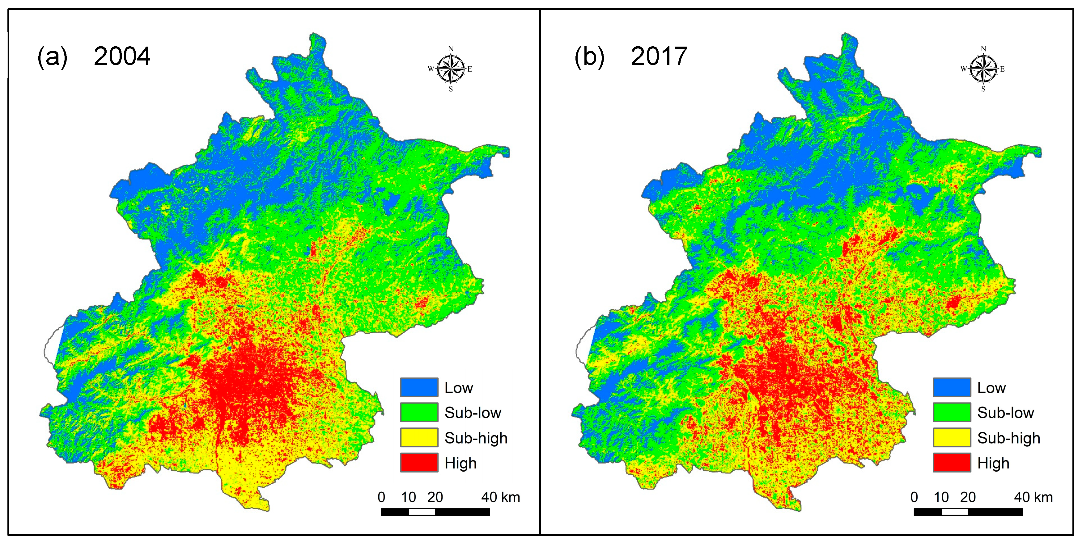
3.1. Urban Land Surface Temperature Dynamics

In 2004, the temperature range of Beijing LST was 19.41–40.98 °C, with an average temperature of 26.12 °C. In 2017 the temperature range of Beijing LST was 13.62–49.65 °C, with an average temperature of 27.88 °C (Figure 3). Figure 4 illustrates the spatial pattern of Beijing’s surface temperature in 2004 and 2017, an obvious high-temperature area appeared in the main urban zone and urban function extended zone, which showed a monocentric spatial pattern. By 2017, there was still an obvious high-temperature area in the main urban zone and urban functional extended zone, and the HTCs had spread to the far suburb zone and new urban development zone, which was related to the process of urban expansion, and showed a significant polycentric spatial pattern.

3.1.1. High Temperature Center Variation of Different Administrative Zones

Table 4. Mean land surface temperature, percentage of high-temperature center, and distribution index in four functional zones between 2004 and 2017.

Zone 1	Year	Mean LST (°C)	Percentage of HTC	DI
MUZ	2004	34.92	85.91%	6.96
	2017	34.13	84.70%	6.17
UFEZ	2004	31.61	58.12%	4.71
	2017	32.01	49.94%	3.64
NUDZ	2004	28.23	17.49%	1.42
	2017	29.86	20.03%	1.46
FSZ	2004	24.35	1.96%	0.16
	2017	26.32	3.07%	0.22
Beijing	2004	26.21	12.34%	-
	2017	27.88	13.72%	-

¹ MUZ, UFEZ, NUDZ, and FSZ represent the main urban zone, urban function extended zone, new urban development zone, and far suburb zone, respectively.

lists the results of distribution index (DI) and proportion of high-temperature centers (HTC) in different administrative zones in 2004 and 2017. The proportion of HTCs in Beijing was 12.34% (2004) and 13.72% (2017), and the average temperature was 26.12 °C (2004) and 27.88 °C (2017). In 2004, Beijing’s HTCs were mainly concentrated in the main urban zone (85.19%) and urban functional extended zone (58.12%). Spatially, the distribution of HTCs tended to decrease from the main urban zone to the suburbs. In 2017, the proportion of HTCs the main urban zone (84.7%) and urban function extended zone (49.94%) were relatively reduced, while the new urban development zone and far suburb zone increased to 20.03% and 3.07%, respectively. The variations of HTC indicated a significant outward spread tendency, which was consistent with the direction of urban (impervious surface) expansion (Figure 2), and the DI value gradually decreased from the main urban zone to the far suburb zone. In 2017, the DI value of the new urban development zone and the far suburb zone increased, while the main urban zone and the urban functional extended zone relatively reduced, which revealed the trend of the HTC gradually expanding to the surrounding zone of urban. Among the four functional zones, only the far suburbs have a DI value of less than 1, indicating that the HTC distribution is lower than the mean level of Beijing and has a cooling effect on urban LST.

3.1.2. High Temperature Center Variation of Different Land Cover Types

Table 5. Mean land surface temperature, percentage of high-temperature center, and distribution index for each landscape type between 2004 and 2017.

Landscape Type	Year	Mean LST (°C)	Percentage of HTC	DI
Impervious surface	2004	31.08	53.74%	4.35
	2017	31.84	47.39%	3.45
Bare land	2004	28.36	12.30%	1.92
	2017	27.74	9.71%	1.26
Cultivated land	2004	27.66	12.67%	1.03
	2017	29.21	11.96%	0.87
Urban green space	2004	28.74	24.04%	1.95
	2017	28.19	7.79%	1.17
Water	2004	26.64	12.34%	0.86
	2017	27.09	5.22%	0.38
Forest	2004	24.29	23.08%	0.19
	2017	25.68	1.01%	0.07

lists the results of distribution index (DI) and proportion of HTCs in different land cover types. The mean LST of impervious surface was the highest (31.08 °C in 2004 and 31.84 °C in 2017), while the lowest in forest land (24.29 °C in 2004 and 25.68 °C in 2017). The DI values of impervious surface and bare land were higher than 1 (4.35, 1.92 in 2004 and 3.45, 1.26 in 2017, respectively), which have a positive contribution to urban LST. The DI values of forest land, water, and cultivated land were less than or close to 1 (0.19, 0.86, 1.03 in 2004 and 0.07, 0.38, 0.87 in 2017, respectively), which have a cooling effect on urban LST. The DI values of water and cultivated land were higher than that of forest land, mainly because water has a higher specific heat capacity and radiation relative to forest land, and is easily affected by the surrounding impervious surface; soil was exposed to the air after crop harvested, which increased the LST of cultivated land. Generally, an obvious cooling effect should exist in the urban green space, and a DI value less than 1, however, the actual value was 1.95 in 2004 and 1.17 in 2017, mainly because Beijing’s green space patches are relatively small and scattered, when the high-temperature air of the impervious surface flows to the green space, after the green space absorbed the surrounding heat, the temperature gradually rises, and the DI value was higher than 1.

3.2. Wavelet Coherency Analysis of Landscape Metrics and Land Surface Temperature

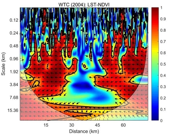
3.2.1. The Wavelet Coherencies between Landscape Composition and Land Surface Temperature

The correlations between NDBI and LST exhibited significant multi-scale characteristics (Figure 5). In 2004, there was no significant correlation between NDBI and LST at smaller scales (less than 0.24 km). With the increase of scales, several regions with a strong correlation began to appear at the scale of 0.24–4.82 km (mainly concentrated in areas with large NDBI values) and varied with spatial location. The correlation was relatively low around 30 and 45 km of the transect, mainly due to the existence of large area urban green space and water in this zone. When the scale exceeds 4.82 km, NDBI was positively correlated with LST on the whole transect, which has a warming effect on LST. In 2017, at smaller scales, the correlation of NDBI and LST tended to increase compared with that in 2004. The correlation mainly distributed at 0–30 km and 45–75 km as the scale increased to 0.48–7.68 km. At the scales over 10.86 km, the whole transects showed a strong positive correlation between NDBI and LST. The scale of low correlation near urban areas increased in 2017, mainly because the increase of impervious surface makes the distribution of urban green space and water more fragmented, which increased the scale where NDBI and LST showed a significant positive correlation in the whole transect.

There showed a strong multi-scale correlation between NDVI and LST (Figure 5). In 2004, NDVI and LST showed a weak correlation at small scales (less than 0.24 km). At the scale of 0.24–0.96 km, a strong correlation begins to appear at several locations. At the scale of 0.96–7.68 km, there was a strong negative correlation in the range of 0–30 km and 50–75 km of the transect, while there was no significant correlation between 30 and 50 km (urban area), probably because the area of vegetation patches in the urban area was small and scattered, which made the NDVI value relatively low and the impact on LST was not obvious. When the scale exceeds 10.68 km, NDVI was negatively related to LST significantly on the whole transect, and has a cooling effect on LST. In 2017, the correlation between NDVI and LST on the scale of 0.96–10.68 km showed the same distribution characteristics as that in 2004. The difference is that when the scale is less than 0.96 km, the whole transects showed a strong negative correlation except several locations. It shows that at larger scales, the vegetation in the two-stage transect data has similar spatial distribution characteristics. The large difference below 0.96 km was probably because the government has built some recreational facilities, green belts, and parks to reduce the impact of urban heat islands on the living environment (for example, in order to host the 2008 Beijing Olympics, the government built the Olympic Park and some green belts to increase urban green space). These urban green space patches are small and scattered in the city, and have a large impact on the land surface temperature at small scales.

The multi-scale correlation between SHDI and LST was weaker than the other two landscape composition indices (Figure 5). At scales less than 3.84 km, wavelet coherent diagrams in 2004 and 2017 have significant correlations only at several locations. At scales of 3.84–15.36 km, there was a significant negative correlation in the urban area. In 2017, the correlation between SHDI and LST showed similar distribution characteristics to that of 2004, although the correlation area and location have expanded. Affected by the patch size of land cover types, the diversity increases first and then decreases with the change of scales. At the scale of 3.84–15.36 km, land cover types in urban areas presented higher diversity, and different land surface radiation within different land use types caused the various temperature distributions in these lands. The unbalanced distribution of LST in space accelerated the flow of land surface air and reduced the LST, which caused a significant negative correlation between SHDI and LST.

3.2.2. The Wavelet Coherencies between Landscape Configuration and Land Surface Temperature

There was no significant correlation between landscape configuration indexes and LST at smaller scales, while at larger scales there was a strong correlation in the urban area (Figure 6). In 2004, the wavelet coherent diagram between CONTAG index and LST showed a strong positive correlation in the urban area at scales of 3.84–15.36 km, mainly because the impervious surfaces were the dominant patches, with high density and connectivity, the CONTAG index was larger in the urban area, and the large area of the impervious surface reduced the diffusion speed of LST. In 2017, the regions with strong positive correlations at these scales expand to both sides, which was the same trend as urban impervious surface expansion. For the DIVISION index, in 2004, there was a strong negative correlation in the urban area at the scales of 7.68–15.36 km. In 2017, the region with strong negative correlation expanded and the scale range increased to 3.84–15.36 km, probably because the urban land cover can be divided into several patches, which increased the diversity, and contributes to the diffusion of LST. For the LSI index, in 2004, a strong negative correlation was identified in the urban area at scales of 3.84–15.36 km. In 2017, the region with strong positive correlation expanded, mainly due to the expansion of the impervious surface, and the degree of fragmentation of the landscape and the complexity of the land type increased, conducive to spreading LST. In general, the influence of landscape configuration metrics on LST at small and medium scales were more complicated, and the opposite correlation characteristics may occur due to location. With the increase of scales, the correlation was more stable and significant.

3.3. Pearson Correlation Coefficient on Different Analysis Scales

Figure 7 and Figure 8 show the Pearson correlation coefficient and wavelet coherence coefficient between landscape metrics and LST at multi-scales. The Pearson coefficient was calculated by the spatial rectangle sampling method, the rectangle size was set to the scale of the Y-axis of the wavelet coherence diagram (eight main scales were selected as an example), and the correlation coefficients at different scales was obtained by spatial the rectangle on the whole transect. At small scales, the rectangle used in calculating the Pearson coefficient was smaller, so that the correlation coefficient at different positions had large fluctuations, but the wavelet coherence coefficient was relatively smooth due to the smoothing operator of scale and position. With the increase of the scale, the Pearson correlation coefficient and the wavelet coherence coefficient have the same trend, although they had some fluctuations in several locations. The Pearson correlation coefficient still has jagged fluctuations at larger scales, while the wavelet coherence coefficient was smoother and closer to a straight line, which better reflected the true correlation between landscape metrics and LST. In general, at large scales, the correlation trends obtained by the two methods were similar, but the Pearson correlation coefficient calculated by the spatial rectangle sampling method was easily affected by the rectangle size and position, while the wavelet coherence was less affected by these factors. Wavelet coherence can better reveal the correlation between LST and landscape metrics at different scales and locations.

4. Discussion

In the past few decades, the accelerated urbanization of Beijing has rapidly increased the impervious surfaces such as roads, squares, and built-up land, which has dramatically changed the urban thermal environment [53]. To mitigate these problems, the satellite city development plans were proposed by government and urban planners to form a polycentric spatial pattern [9], as reflected in the land cover and LST maps of 2004–2017. In 2004, the high-temperature center of Beijing was concentrated in the main urban zone and urban function extended zone. In 2017, the high-temperature center was gradually spread to the peripheral urban zone, which made the thermal environment of the main urban zone improve apparently. In addition, according to the Beijing Urban Master Plan 2004–2020, the government has built some parks and green belts around the urban area to increase the urban green space and ameliorate the LST in the urban area [39]. NDVI and LSI showed a strong negative correlation at small scales in 2017, which also revealed the phenomenon of increased urban green space. However, with the in-filling development pattern between urban polycentric, most lands between the satellite city and the main urban zone were used for commercial finance and residential, and only smaller and scattered land were used for urban green space. The impervious surface was gradually connected, which may have an adverse effect on the urban thermal environment.

The significant impact of urban local thermal environment on urban ecology made it an obligation to understand the changes in land cover and spatial pattern of LST [54]. Previous studies have shown that LST were affected by a variety of factors, such as urban structure, land cover types, geographic location, and population [13,55,56]. Land cover type is one of the main factors affecting LST, compared to areas with abundant land cover types (especially the land types which could adjust the LST, such as water and vegetation), the single and continuous impervious surface contributes more to the urban LST. The water and vegetation in the Beijing urban zone are smaller and fragmented, showed a negative correlation with LST at small and medium scales, and have a cooling effect. While at large scales, the impermeable surface is the dominant patch with a significant positive correlation with LST, which reduced the cooling effect of water and vegetation. The spatial configuration indexes of the main urban area have a strong correlation with LST at large scales. Urbanization has increased the fragmentation of the Beijing landscape, and the urban land cover types have become more diverse and complex, which may be helpful to mitigate the LST in urban areas [29,38]. In addition, LST images obtained at different times are also affected by atmospheric radiation, solar radiation, wind speed, humidity, etc. The LST data obtained in 2004 and 2017 may not have been stable, which will have a certain effect on the analysis of the spatial pattern distribution characteristics of LST [57]. In this paper, the two LST data were selected at the beginning and end of Beijing’s urban master plan (2004–2020), which represented the process of urban development of Beijing cities during a completed master plan period. The two periods of data sets provide the vision to investigate the process of land use change and the correlation of the corresponding temperature gradient during the pursuit of the 2004–2017 master plan. In addition, this paper focuses on the multi-scale correlation between landscape index (landscape composition and spatial configuration) and the land surface temperature, and the two periods of data for subsequent wavelet coherent analysis are also helpful for the scale variation between the two periods.

The Pearson correlation diagram obtained by the spatial rectangle sampling at different locations and scales showed a similar trend to wavelet coherence, and the undulated tendency was mainly caused by the calculation of rectangle size and pixel size. In contrast, the wavelet coherent diagram was relatively smooth and less affected by the above factors, which was consistent with the real situation of the impact of landscape metrics on LST, and proved the effectiveness and adaptability of wavelet coherence in the multi-scale analysis. Although wavelet coherence provides a new perspective for multi-scale identification of the correlation between LST and landscape pattern, several deficiencies still existed. For example, the window size selected when calculating various types of landscape indices at the landscape level, and the transect selected when analyzing the correlation between the landscape index and the LST, these factors will inevitably affect the analysis results. Moreover, the ecological interpretation of wavelet coherent diagram is complex, and the scale needs to be more accurately and finely divided. Considering the diurnal and seasonal variation of temperature, the sensitivity of different indexes to the LST, as well as the impact of more time-series of LST images on the analysis results, more LST images, more effective landscape indexes, and precise scales may be applied in the future to study the LST dynamic and the correlation between urban landscape pattern and LST.

5. Conclusions

This study applied wavelet coherence and Pearson correlation coefficient to analyze the multi-scale correlations between landscape pattern and LST, and analyzed the spatial pattern of the urban thermal environment during the urbanization of the Beijing from 2004 to 2017 using the distribution index of high-temperature centers. According to the experimental results, we drew the following conclusions:

• The HTC of Beijing has a tendency to spread outwards from 2004 to 2017. In 2004, it mainly concentrated in the main urban zone and urban function extended zone, forming a spatial pattern of monocenter distribution. In 2017, the HTC gradually expanded to the new urban development zone and far suburb zone, with a spatial pattern of polycentric distribution, and gradually connected to the main urban zone and urban function extended zone, which has an adverse effect on urban LST.
• Land cover types have a significant impact on the spatial pattern of LST. The mean LST and HTC distribution of the impervious surface were the highest, while the forest land and water body were lower. Urban green space has a cooling effect on the LST, but due to its small area and scattered distribution, easily affected by the large-area impervious surface, causing the mean temperature and HTC distribution to be higher than forest land and water body.
• Wavelet coherent analysis showed that the correlation between landscape pattern metrics (landscape composition and configuration) and LST has significant multi-scale effects. The landscape composition indices NDBI and NDVI showed a correlation with LST at all scales, especially at large scales, which showed a strong positive correlation and negative correlation, respectively. The space configuration indices CONTAG, DIVISION, and LSI have no significant correlation with LST at smaller scales. With the increase of scale, it showed a strong correlation around the urban area.
• The wavelet coherence and Pearson correlation coefficients showed that the landscape composition and spatial configuration have significant effects on the LST, but the landscape composition has a greater impact on the LST in the Beijing metropolitan area.
• Totally, compared with Pearson correlation coefficient calculated by spatial rectangle sampling, the wavelet coherence diagram is smoother and less affected by the location and rectangle size, which is more conducive to describing the correlation between landscape pattern index and LST at different scales and locations.

References

1. Foster, S.S.D. The interdependence of groundwater and urbanisation in rapidly developing cities. Urban Water 2001, 3, 185–192. [Google Scholar] [CrossRef]
2. Seto, K.C.; Sánchez-Rodríguez, R.; Fragkias, M. The New Geography of Contemporary Urbanization and the Environment. Annu. Rev. Environ. Resour. 2010, 35, 167–194. [Google Scholar] [CrossRef] [Green Version]
3. Siswanto, S.; van Oldenborgh, G.J.; van der Schrier, G.; Jilderda, R.; van den Hurk, B. Temperature, extreme precipitation, and diurnal rainfall changes in the urbanized Jakarta city during the past 130 years. Int. J. Climatol. 2016, 36, 3207–3225. [Google Scholar] [CrossRef]
4. Mander, Ü.; Kull, A.; Tamm, V.; Kuusemets, V.; Karjus, R. Impact of climatic fluctuations and land use change on runoff and nutrient losses in rural landscapes. Landsc. Urban Plan. 1998, 41, 229–238. [Google Scholar] [CrossRef]
5. Luck, M.; Wu, J. A gradient analysis of urban landscape pattern: a case study from the Phoenix metropolitan region, Arizona, USA. Landsc. Ecol. 2002, 17, 327–339. [Google Scholar] [CrossRef]
6. Peng, J.; Liu, Z.; Liu, Y.; Wu, J.; Han, Y. Trend analysis of vegetation dynamics in Qinghai–Tibet Plateau using Hurst Exponent. Ecol. Indic. 2012, 14, 28–39. [Google Scholar] [CrossRef]
7. Li, J.; Li, C.; Zhu, F.; Song, C.; Wu, J. Spatiotemporal pattern of urbanization in Shanghai, China between 1989 and 2005. Landsc. Ecol. 2013, 28, 1545–1565. [Google Scholar] [CrossRef]
8. Arnfield, A.J. Two decades of urban climate research: a review of turbulence, exchanges of energy and water, and the urban heat island. Int. J. Climatol. 2003, 23, 1–26. [Google Scholar] [CrossRef]
9. Peng, J.; Xie, P.; Liu, Y.; Ma, J. Urban thermal environment dynamics and associated landscape pattern factors: A case study in the Beijing metropolitan region. Remote Sens. Environ. 2016, 173, 145–155. [Google Scholar] [CrossRef]
10. Song, J.; Du, S.; Feng, X.; Guo, L. The relationships between landscape compositions and land surface temperature: Quantifying their resolution sensitivity with spatial regression models. Landsc. Urban Plan. 2014, 123, 145–157. [Google Scholar] [CrossRef]
11. Ma, Q.; Wu, J.; He, C. A hierarchical analysis of the relationship between urban impervious surfaces and land surface temperatures: Spatial scale dependence, temporal variations, and bioclimatic modulation. Landsc. Ecol. 2016, 31, 1139–1153. [Google Scholar] [CrossRef]
12. Berger, C.; Rosentreter, J.; Voltersen, M.; Baumgart, C.; Schmullius, C.; Hese, S. Spatio-temporal analysis of the relationship between 2D/3D urban site characteristics and land surface temperature. Remote Sens. Environ. 2017, 193, 225–243. [Google Scholar] [CrossRef]
13. Zhou, W.; Huang, G.; Cadenasso, M.L. Does spatial configuration matter? Understanding the effects of land cover pattern on land surface temperature in urban landscapes. Landsc. Urban Plan. 2011, 102, 54–63. [Google Scholar] [CrossRef]
14. Li, X.; Zhou, W.; Ouyang, Z.; Xu, W.; Zheng, H. Spatial pattern of greenspace affects land surface temperature: evidence from the heavily urbanized Beijing metropolitan area, China. Landsc. Ecol. 2012, 27, 887–898. [Google Scholar] [CrossRef]
15. Gustafson, E.J. Quantifying Landscape Spatial Pattern: What Is the State of the Art? Ecosystems 1998, 1, 143–156. [Google Scholar] [CrossRef]
16. Du, S.; Xiong, Z.; Wang, Y.-C.; Guo, L. Quantifying the multilevel effects of landscape composition and configuration on land surface temperature. Remote Sens. Environ. 2016, 178, 84–92. [Google Scholar] [CrossRef]
17. Owen, T.W.; Carlson, T.N.; Gillies, R.R. An assessment of satellite remotely-sensed land cover parameters in quantitatively describing the climatic effect of urbanization. Int. J. Remote Sens. 1998, 19, 1663–1681. [Google Scholar] [CrossRef]
18. Streutker, D.R. Satellite-measured growth of the urban heat island of Houston, Texas. Remote Sens. Environ. 2003, 85, 282–289. [Google Scholar] [CrossRef]
19. Frey, C.M.; Rigo, G.; Parlow, E. Urban radiation balance of two coastal cities in a hot and dry environment. Int. J. Remote Sens. 2007, 28, 2695–2712. [Google Scholar] [CrossRef]
20. Xie, M.; Wang, Y.; Chang, Q.; Fu, M.; Ye, M. Assessment of landscape patterns affecting land surface temperature in different biophysical gradients in Shenzhen, China. Urban Ecosyst. 2013, 16, 871–886. [Google Scholar] [CrossRef]
21. Yuan, F.; Bauer, M.E. Comparison of impervious surface area and normalized difference vegetation index as indicators of surface urban heat island effects in Landsat imagery. Remote Sens. Environ. 2007, 106, 375–386. [Google Scholar] [CrossRef]
22. Sun, R.; Chen, A.; Chen, L.; Lü, Y. Cooling effects of wetlands in an urban region: The case of Beijing. Ecol. Indic. 2012, 20, 57–64. [Google Scholar] [CrossRef]
23. Connors, J.P.; Galletti, C.S.; Chow, W.T.L. Landscape configuration and urban heat island effects: assessing the relationship between landscape characteristics and land surface temperature in Phoenix, Arizona. Landsc. Ecol. 2013, 28, 271–283. [Google Scholar] [CrossRef]
24. Xiao, R.B.; Weng, Q.H.; Ouyang, Z.Y.; Li, W.F.; Schienke, E.W.; Zhang, Z.M. Land surface temperature variation and major factors in Beijing, China. Photogramm. Eng. Remote Sens 2008, 74, 451–461. [Google Scholar]
25. Zhang, X.; Zhong, T.; Feng, X.; Wang, K. Estimation of the relationship between vegetation patches and urban land surface temperature with remote sensing. Int. J. Remote Sens. 2009, 30, 2105–2118. [Google Scholar] [CrossRef]
26. Wu, J. Effects of changing scale on landscape pattern analysis: scaling relations. Landsc. Ecol. 2004, 19, 125–138. [Google Scholar] [CrossRef]
27. Xu, C.; Liu, M.; Hong, C.; Chi, T.; An, S.; Yang, X. Temporal variation of characteristic scales in urban landscapes: an insight into the evolving internal structures of China’s two largest cities. Landsc. Ecol. 2012, 27, 1063–1074. [Google Scholar] [CrossRef]
28. Biswas, A.; Si, B.C. Scales and locations of time stability of soil water storage in a hummocky landscape. J. Hydrol. 2011, 408, 100–112. [Google Scholar] [CrossRef]
29. Guo, L.; Liu, R.; Men, C.; Wang, Q.; Miao, Y.; Zhang, Y. Quantifying and simulating landscape composition and pattern impacts on land surface temperature: A decadal study of the rapidly urbanizing city of Beijing, China. Sci. Total Environ. 2019, 654, 430–440. [Google Scholar] [CrossRef]
30. Dale, M.R.T.; Mah, M. The Use of Wavelets for Spatial Pattern Analysis in Ecology. J. Veg. Sci. 1998, 9, 805–814. [Google Scholar] [CrossRef]
31. Lark, R.M.; Webster, R. Analysis and elucidation of soil variation using wavelets. Eur. J. Soil Sci. 1999, 50, 185–206. [Google Scholar] [CrossRef]
32. Dong, X.; Nyren, P.; Patton, B.; Nyren, A.; Richardson, J.; Maresca, T. Wavelets for Agriculture and Biology: A Tutorial with Applications and Outlook. BioScience 2008, 58, 445–453. [Google Scholar] [CrossRef] [Green Version]
33. Grinsted, A.; Moore, J.C.; Jevrejeva, S. Application of the cross wavelet transform and wavelet coherence to geophysical time series. Nonlin Process. Geophys 2004, 11, 561–566. [Google Scholar] [CrossRef]
34. Vadrevu, K.P.; Choi, Y. Wavelet analysis of airborne CO2 measurements and related meteorological parameters over heterogeneous landscapes. Atmos. Res. 2011, 102, 77–90. [Google Scholar] [CrossRef]
35. Wu, Q.; Guo, F.; Li, H. Wavelet-Based Correlation Identification of Scales and Locations between Landscape Patterns and Topography in Urban-Rural Profiles: Case of the Jilin City, China. Remote Sens. 2018, 10, 1653. [Google Scholar] [CrossRef] [Green Version]
36. Biswas, A. Landscape characteristics influence the spatial pattern of soil water storage: Similarity over times and at depths. CATENA 2014, 116, 68–77. [Google Scholar] [CrossRef]
37. Saunders, S.C.; Chen, J.; Drummer, T.D.; Gustafson, E.J.; Brosofske, K.D. Identifying scales of pattern in ecological data: a comparison of lacunarity, spectral and wavelet analyses. Ecol. Complex. 2005, 2, 87–105. [Google Scholar] [CrossRef]
38. Qiao, Z.; Tian, G.; Xiao, L. Diurnal and seasonal impacts of urbanization on the urban thermal environment: A case study of Beijing using MODIS data. Isprs J. Photogramm. Remote Sens. 2013, 85, 93–101. [Google Scholar] [CrossRef]
39. Jiang, G.; Ma, W.; Qu, Y.; Zhang, R.; Zhou, D. How does sprawl differ across urban built-up land types in China? A spatial-temporal analysis of the Beijing metropolitan area using granted land parcel data. Cities 2016, 58, 1–9. [Google Scholar] [CrossRef]
40. Meng, Q.; Zhang, L.; Sun, Z.; Meng, F.; Wang, L.; Sun, Y. Characterizing spatial and temporal trends of surface urban heat island effect in an urban main built-up area: A 12-year case study in Beijing, China. Remote Sens. Environ. 2018, 204, 826–837. [Google Scholar] [CrossRef]
41. Barsi, J.A.; Schott, J.R.; Palluconi, F.D.; Heider, D.L.; Hook, S.J.; Markham, B.L.; Chander, G.; O'Donnell, E.M. Landsat TM and ETM+ thermal band calibration. Can. J. Remote Sens 2003, 29, 141–153. [Google Scholar]
42. Liu, L.; Zhang, Y. Urban Heat Island Analysis Using the Landsat TM Data and ASTER Data: A Case Study in Hong Kong. Remote Sens. 2011, 3, 1535–1552. [Google Scholar] [CrossRef] [Green Version]
43. Chander, G.; Groeneveld, D.P. Intra-annual NDVI validation of the Landsat 5 TM radiometric calibration. Int. J. Remote Sens. 2009, 30, 1621–1628. [Google Scholar] [CrossRef]
44. Chander, G.; Markham, B.L.; Helder, D.L. Summary of current radiometric calibration coefficients for Landsat MSS, TM, ETM+, and EO-1 ALI sensors. Remote Sens. Environ. 2009, 113, 893–903. [Google Scholar] [CrossRef]
45. Artis, D.A.; Carnahan, W.H. Survey of emissivity variability in thermography of urban areas. Remote Sens. Environ. 1982, 12, 313–329. [Google Scholar] [CrossRef]
46. Weng, Q.; Liu, H.; Liang, B.; Lu, D. The Spatial Variations of Urban Land Surface Temperatures: Pertinent Factors, Zoning Effect, and Seasonal Variability. Ieee J. Sel. Top. Appl. Earth Obs. Remote Sens. 2008, 1, 154–166. [Google Scholar] [CrossRef]
47. Li, J.; Song, C.; Cao, L.; Zhu, F.; Meng, X.; Wu, J. Impacts of landscape structure on surface urban heat islands: A case study of Shanghai, China. Remote Sens. Environ. 2011, 115, 3249–3263. [Google Scholar] [CrossRef]
48. Azhdari, A.; Soltani, A.; Alidadi, M. Urban morphology and landscape structure effect on land surface temperature: Evidence from Shiraz, a semi-arid city. Sustain. Cities Soc. 2018, 41, 853–864. [Google Scholar] [CrossRef]
49. Kumar, P.; Foufoula-Georgiou, E. Wavelet analysis for geophysical applications. Rev. Geophys. 1997, 35, 385–412. [Google Scholar] [CrossRef] [Green Version]
50. Farge, M. WAVELET TRANSFORMS AND THEIR APPLICATIONS TO TURBULENCE. Annu. Rev. Fluid Mech. 1992, 24, 395–458. [Google Scholar] [CrossRef]
51. Torrence, C.; Compo, G.P. A Practical Guide to Wavelet Analysis. Bull. Am. Meteorol. Soc. 1998, 79, 61–78. [Google Scholar] [CrossRef] [Green Version]
52. Si, B.C.; Zeleke, T.B. Wavelet coherency analysis to relate saturated hydraulic properties to soil physical properties. Water Resour. Res. 2005, 41. [Google Scholar] [CrossRef]
53. Wang, J.; Zhou, W.; Pickett, S.T.A.; Yu, W.; Li, W. A multiscale analysis of urbanization effects on ecosystem services supply in an urban megaregion. Sci. Total Environ. 2019, 662, 824–833. [Google Scholar] [CrossRef] [PubMed]
54. Turner, B.L.; Lambin, E.F.; Reenberg, A. The emergence of land change science for global environmental change and sustainability. Proc. Natl. Acad. Sci. 2007, 104, 20666. [Google Scholar] [CrossRef] [PubMed] [Green Version]
55. Taha, H. Urban climates and heat islands: albedo, evapotranspiration, and anthropogenic heat. Energy Build. 1997, 25, 99–103. [Google Scholar] [CrossRef] [Green Version]
56. Zhang, H.; Qi, Z.-F.; Ye, X.-Y.; Cai, Y.-B.; Ma, W.-C.; Chen, M.-N. Analysis of land use/land cover change, population shift, and their effects on spatiotemporal patterns of urban heat islands in metropolitan Shanghai, China. Appl. Geogr. 2013, 44, 121–133. [Google Scholar] [CrossRef]
57. Dissanayake, D.; Morimoto, T.; Ranagalage, M.; Murayama, Y. Land-Use/Land-Cover Changes and Their Impact on Surface Urban Heat Islands: Case Study of Kandy City, Sri Lanka. Climate 2019, 7, 99. [Google Scholar] [CrossRef] [Green Version]
Figure 1. Study area. Four functional zones of Beijing, including the main urban area (MUZ), urban function extended zone (UFEZ), new urban development zone (NUDZ), and far suburb zone (FSZ).
Remotesensing 11 03021 g001
Figure 2. Land cover maps with a spatial resolution of 30 m. (a) Land cover map for 2004; (b) land cover map for 2017; (c) selected transect (black rectangular zone) for wavelet coherence analysis. The transect spanned the central axis of Beijing from north to south with all land cover types and complex landscape patterns to scrutinize the fine correlation between landscape index and land surface temperature (LST).
Remotesensing 11 03021 g002
Figure 3. The land surface temperature maps of 2004 and 2017.
Remotesensing 11 03021 g003
Figure 4. The land surface temperature classification maps of 2004 and 2017.
Remotesensing 11 03021 g004
Figure 5. The wavelet coherency diagram of landscape composition indexes and land surface temperatures for 2004 and 2017. In the wavelet coherence diagram, the X-axis represents the spatial position; the Y-axis represents the scale obtained from the correlation period; the solid black line represents the influence cone (COI); the thick black line represents the 95% confidence level; the arrow direction indicates the type of correlation, the arrow to the left indicates a negative correlation, while the arrow to the right indicates a positive correlation.
Remotesensing 11 03021 g005
Figure 6. The wavelet coherency diagram of landscape configuration indexes and land surface temperatures for 2004 and 2017.
Remotesensing 11 03021 g006
Figure 7. (a) The Pearson correlation coefficient and wavelet coherence coefficient between NDBI and LST. (b) The Pearson correlation coefficient and wavelet coherence coefficient between NDVI and LST.
Remotesensing 11 03021 g007
Figure 8. (a) The Pearson correlation coefficient and wavelet coherence coefficient between DIVISION and LST. (b) The Pearson correlation coefficient and wavelet coherence coefficient between LSI and LST.
Remotesensing 11 03021 g008