In this Section, the statistical description of the enhanced noise-filtered phase estimator shown in Equation (4) is first inferred. Subsequently, some insights on the calculation of the matrix covariance of the reconstructed interferograms are theoretically derived, thus emphasizing the role of the exploited time-redundant network of InSAR interferograms and the benefit of pre-selecting only small baseline (SB) interferograms during the optimization procedure.
3.1. Directional Statistics
As earlier anticipated in
Section 2, the E-MTInSAR noise-filtering technique is based on the solution of a non-linear optimization problem, which is independently computed for every radar pixel of the imaged scene and consists of searching for the phase vector of wrapped phases
that minimize the (weighted) circular variance of the random (wrapped) phase vector
. The vector of weights
in (4) represents our confidence in the quality of the exploited, original
M (small baseline) multi-looked interferograms. To this aim, the spatial coherence factor of each relevant interferograms is used. In particular, the latter is computed directly from the phase of the original multi-looked interferograms, see [
26], as follows:
where 2
NA+1 and 2
NR+1 represent the number of azimuth and range pixels within the used boxcar averaging window, which is centered around the generic pixel of radar coordinates (
x,
r). Because the amplitude and phase of SAR images can be assumed as independent random signals, it can be proven [
13] that the coherence estimated via Equation (6) is an unbiased estimator of the actual spatial coherence, which is defined as follows [
13]:
where
IIMk and
IISk are the complex-valued master and slave images involved in the generation of the
k-th InSAR differential interferogram, respectively, and the symbol
E[·] represents the statistical expectation operator.
The basic principle of the proposed noise-filtering technique consists in the minimization of the (weighted) circular variance [
26,
29], namely
ν, of the random circular data
. The circular variance is calculated as follows [
29]:
with
ρ being the sampled (measured) weighted mean resultant length
of the circular data
, which represents the amplitude of the following complex term:
where:
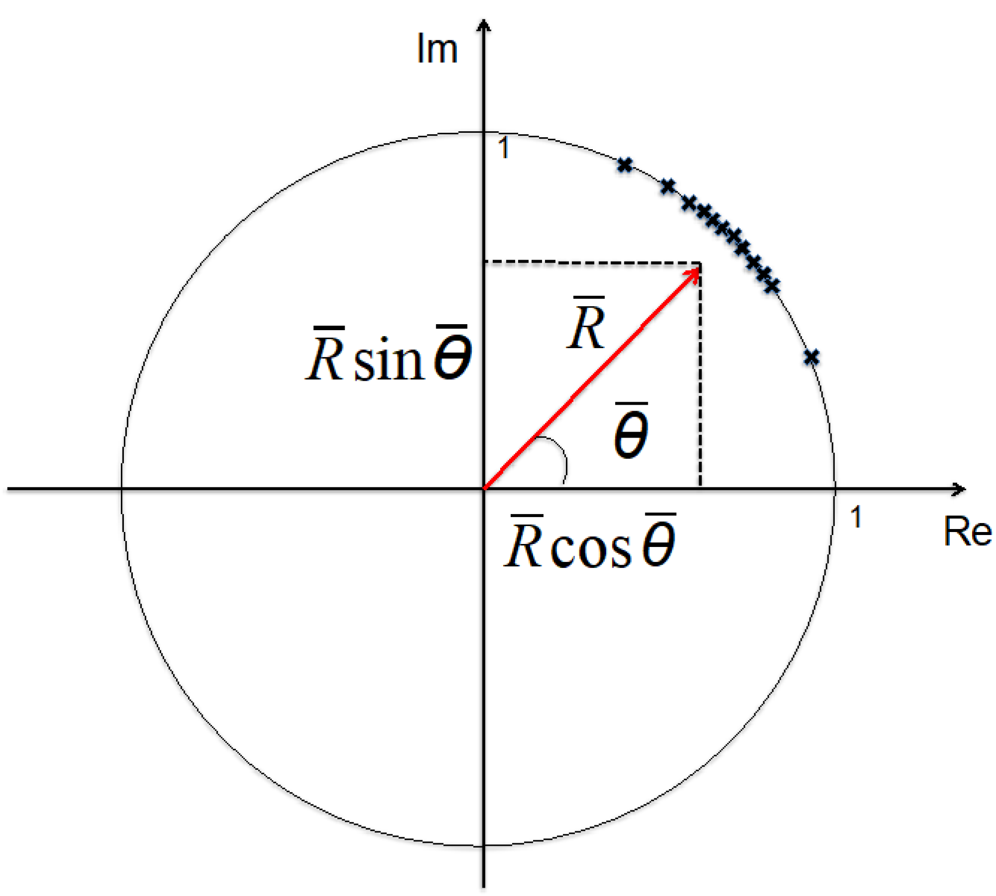
Taking into account Equation (10), see also
Figure 1, it is straightforward to prove (see Mardia’s book [
29] for additional details) that:
Accordingly, Equation (8) can be conveniently re-written as follows:
It is worthwhile to note that the minimization of the circular variance of the random vector Θ leads to the minimal dispersion of the directional data Θ with respect to the (weighted) mean direction has also been proven.
In this research, one of the main goals is to evaluate the statistical characteristics of the directional phase residuals after the non-linear optimization in Equations (4) and (12).
The first issue is the statistical description of the (weighted) resultant length
and the (weighted) mean direction
. For the sake of simplicity, let us initially assume that the used weights
are non-random terms (even though a generalization to the case of random independent variables leads to the same global results), and calculate the statistical average and the standard deviation of
and
. Let us start by considering the first statistical moments of
[
29]:
It is realistic to assume that, after the application of the non-linear optimization procedure in (12), the random residual phase terms
can be seen as independent and identically distributed (i.i.d) random variables. In the literature, the more important families of distribution for data on a circle (i.e., directional data) are the uniform, cardiod, wrapped normal, wrapped Cauchy and von Mises distributions [
29,
36,
37]. From statistical inference, perhaps the most useful distributions on the circle are the von Mises distributions [
38]. Accordingly, in this research paper, I assume the directional data
have a von Mises distribution. This assumption might be tested by considering the statistical tests provided in Reference [
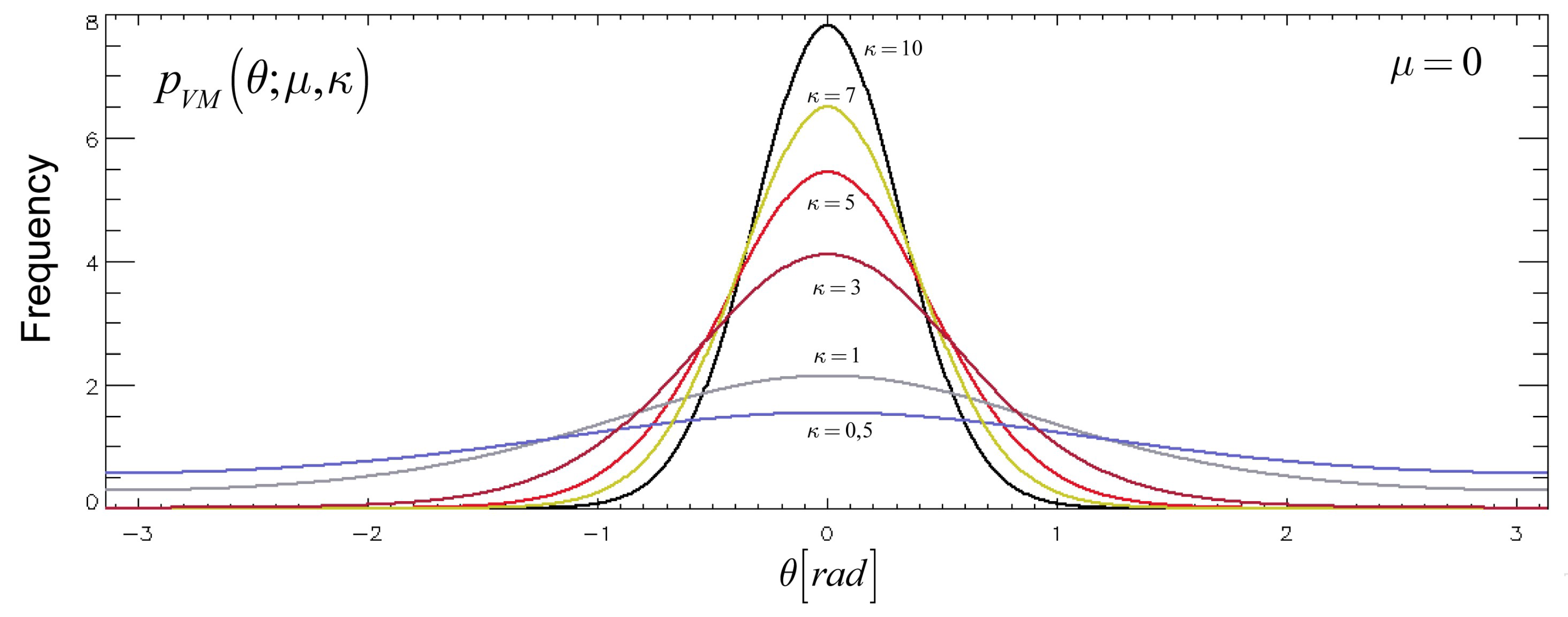
29]. The von Mises distribution has the following probability density function (pdf) [
38]:
where
is the modified Bessel function of the first kind and order zero, see [
39]. The parameter
is the mean direction and
is the concentration parameter. The distribution is unimodal and symmetrical about the direction
. For very small values of the concentration parameter
, the von Mises distribution approximates a uniform distribution whereas, for larger values of the concentration parameter, it tends to become more concentrated at the point
, as shown in
Figure 2.
By assuming that
is a vector of i.i.d random variables with a von Mises distribution with concentration parameter
, the average expectation of the resultant weighted length is as follows:
Noteworthy, the expected (weighted) mean resultant length does not depend on the used weights. This result could seem quite counter-intuitive; however, it proves that, as long as the population is large enough (i.e., in this case, the number of interferograms
), the expected (weighted) circular variance, see also [
26], is the same as the conventional circular variance (with no weights). Conversely, as clarified in the following, the statistics of the reconstructed phase components strictly depend on the used weights.
A suitable expansion of the function
in (15) is as follows [
29]:
As evident, depending on the (measured) value of the resultant mean length , the distribution of the phase is more or less concentrated about its mean direction . In particular, large values of correspond to more concentrated distributions of the phase residuals about their mean (weighted) direction.
Note also that as
, a Von Mises distribution approximates a wrapped normal (WN) distribution. More precisely:
Specifically, the wrapped normal distribution
is obtained by wrapping the normal distribution
, of given mean and standard deviation values
and
, respectively, onto the circle, where
. WN distribution has the following pdf [
29]:
The calculation of the standard deviation of the (weighted) resultant length
is now in order. It is straightforward to demonstrate that, at variance with the expected value, it rigorously depends on the used weights. In fact:
where
and
represent the mean and root mean square (RMS) values of the used weights. For von Mises distributions that are symmetrical about zero, namely
, which is a reasonable assumption in our specific case, it can also be shown that:
The weights significantly modify the standard deviation of the (weighted) mean resultant length. More importantly, it is worth remarking that the standard deviation of the circular variance, see Equation (8), is the same as the standard deviation of the (weighted) resultant length. Accordingly, Equation (20) shows that the adopted estimator in (4) and (12) is an unbiased and consistent estimator of the resultant mean length of the phase population, e.g., its standard deviation tends to zero as the number of samples
. Additionally, by extending the analyses provided in Reference [
29] to the (weighted) circular variance estimator in Equation (4) and (12), it can also be proven that the estimator of the (weighted) mean resultant length is also an efficient estimator. Moreover, for a von Mises distribution, the maximum likelihood estimate (MLE) of the concentration parameter
κ is also carried out as the solution of the following equation:
Solutions of Equation (21) are listed for different ranges of values of the (measured) mean resultant length
ρ of the population. In particular, for
ρ ≥ 0.85, the following relation holds:
Thus, leading one to the possibility of having an MLE estimate of the concentration parameter of the distribution from the measured (optimal) value of the circular variance (see Equations (9) and (12) again).
3.2. Statistical Characterization of the E-MTInSAR Phase Estimator
At this stage, the statistical characterization of the (weighted) mean direction estimator is in order. By the central limit theorem [
40], it can be shown that the joint distribution of
and
is asymptotically normal, and the joint distribution of
and
is asymptotically bivariate.
By extending the work of Reference [
29] (and references therein), the following relations are valid for von Mises distributions that are symmetrical about zero (e.g.,
, as it is expected in our case):
Therefore, the (weighted) mean resultant length and mean direction are asymptotically uncorrelated. By using the MLE value of the concentration parameter
, see Reference (22), and after simple mathematical manipulations, it can be demonstrated that the variances of
and
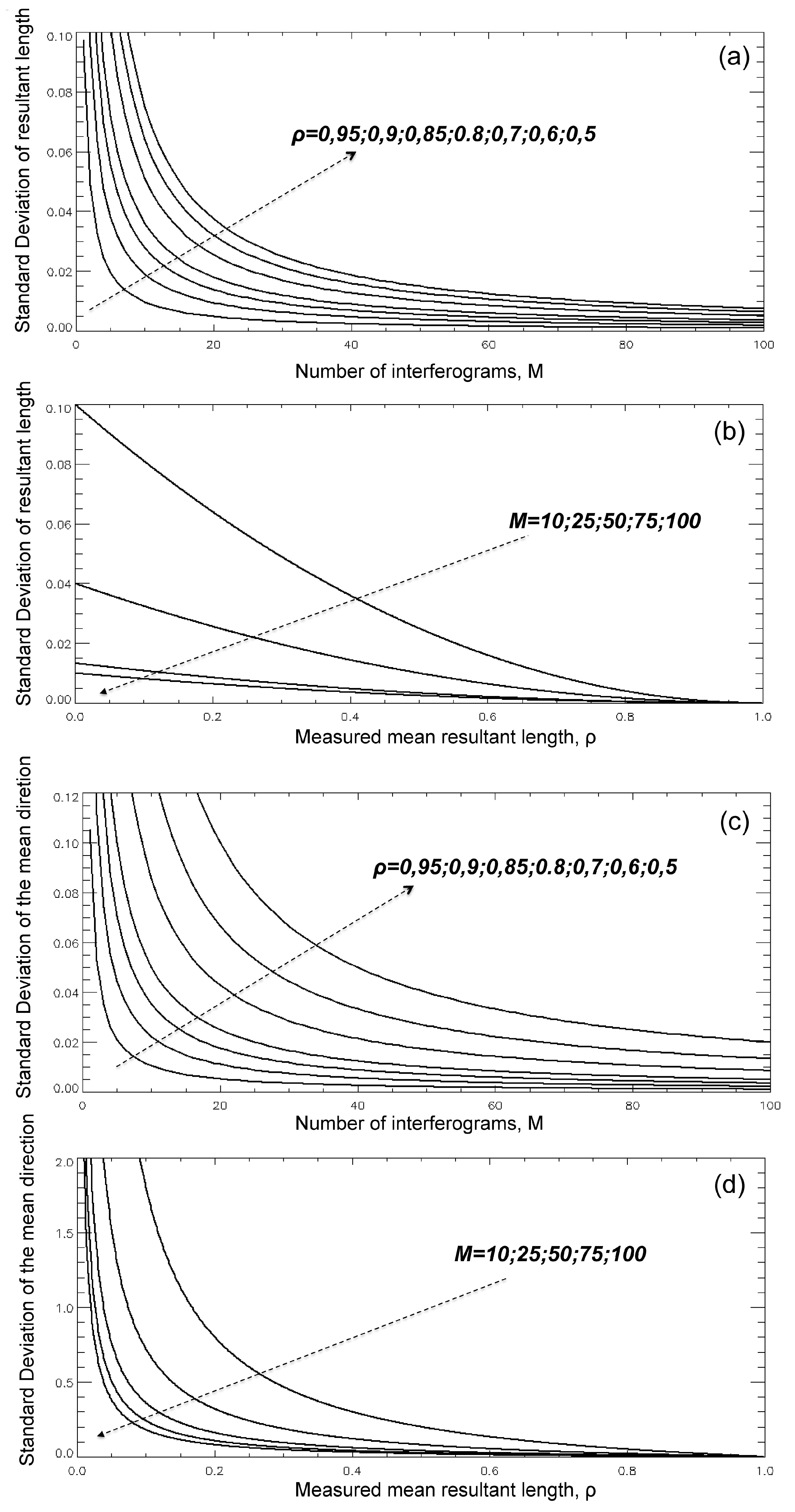
are expressed as follows:
The derivation of Equation (24) is based on the general assumption that the phase is distributed with a von Mises pdf and using Equations (16) and (23) approximated to the first order.
Figure 3 plots the variance of the (weighted) mean resultant length and mean direction of the random phase signal
for different values of the number of interferograms
and the measured value of
. Equation (24) shows that the variance of the (weighted) mean resultant length and (weighted) mean direction can be calculated by the knowledge of the measured (weighted) circular variance value
. An alternative derivation, which takes into account the actual characteristic of the random vector
, representing the phase residuals between the original (unfiltered)
and the reconstructed (filtered)
interferograms, is also provided.
Starting from Equation (12), and using error source propagation rules [
41], the standard deviation of the circular variance estimator of Equation (12) can be calculated as follows:
where
and
are the standard deviation values of the original interferograms and the optimal acquisition phases, respectively, as well as
and
are the corresponding phase co-variance terms. The (weighted) circular variance
depends on the phases of the original interferograms as well as on the reconstructed (unknown) phases of the acquisition dates. It is worth remarking that the non-linear optimization problem in Equation (12) searches for the minimal value of the circular variance; accordingly, the estimated phase values related to every SAR acquisition correspond to a stationary point onto the N-dimensional space of every possible solution, and, as a consequence,
.
Accordingly, Equation (25) simplifies as:
As said, the interferograms are computed after the application of two independent steps: the spatial multi-looking and a (potential) preliminary (single-channel) noise filtering step, performed on every single interferogram (for instance the procedure presented in References [
14,
19]). Although the originally computed interferograms have a given grade of dependence, since they are obtained by the same sequence of SAR data, here I can assume, for the sake of simplicity, that the interferometric phases are uncorrelated. This simplified assumption is widely adopted in the literature, even though very few InSAR studies have addressed the problem of the correlation among a group of InSAR interferograms that are computed from the same set of SAR data [
42]. Accordingly, for statistical inference, I assume that the original interferograms are independent, uncorrelated and with proper standard deviation values. From the literature, it is known that if
is the number of independent looks used during the spatial multi-look operation, and under proper hypotheses on the phase distribution, the standard deviation of the original multi-look interferograms is expressed as follows [
12,
13]:
where the terms
synthetically account for the effects of the potentially used, pre-processing spatial noise-filtered approach, and
are the spatial coherence values of the original interferograms, calculated in correspondence to the radar pixel under investigation. Besides,
represents the number of equivalent looks employed during the multi-looking operation. Moreover, spatial coherence values can be approximated with the estimates provided by Equation (6), used as weights of the solved non-linear optimization problem. Hence, by assuming, in the first instance, that phases are uncorrelated and independent, the co-variance phase terms in Equation (26) vanish, and the following simplified relation holds:
The calculation of the term
is now in order. Starting from Equation 12, after little mathematical manipulations, it is straightforward to demonstrate that:
In the stationary phase condition, i.e., by referring to the optimal circular data retrieved after the solution of the non-linear optimization problem in Equation (4), it is reasonable to approximate the sin functions in Equation (29) with their argument; thus, the following relation is obtained:
and by substitution of Equation (30) into Equation (28), the standard deviation of the phase estimator used within the E-MTInSAR algorithm is finally derived:
where
is the average value of
and
is the root mean square value of the (estimated) coherence. If the resultant mean length
calculated over the optimal phase estimates (i.e., on the circular data
resulting from the optimization procedure) is high, we can assume the phase
is distributed as a wrapped normal (WN), and we can calculate the standard deviation of the residual phase as, see Equation (18),
. However, if we take into account, for the sake of simplicity, only the noise decorrelation artifacts due to the perpendicular baseline of the considered interferograms (i.e., the so-called spatial decorrelation), we also know that spatial coherence
decreases as the perpendicular baseline of the interferograms, namely
, increases [
13]:
where
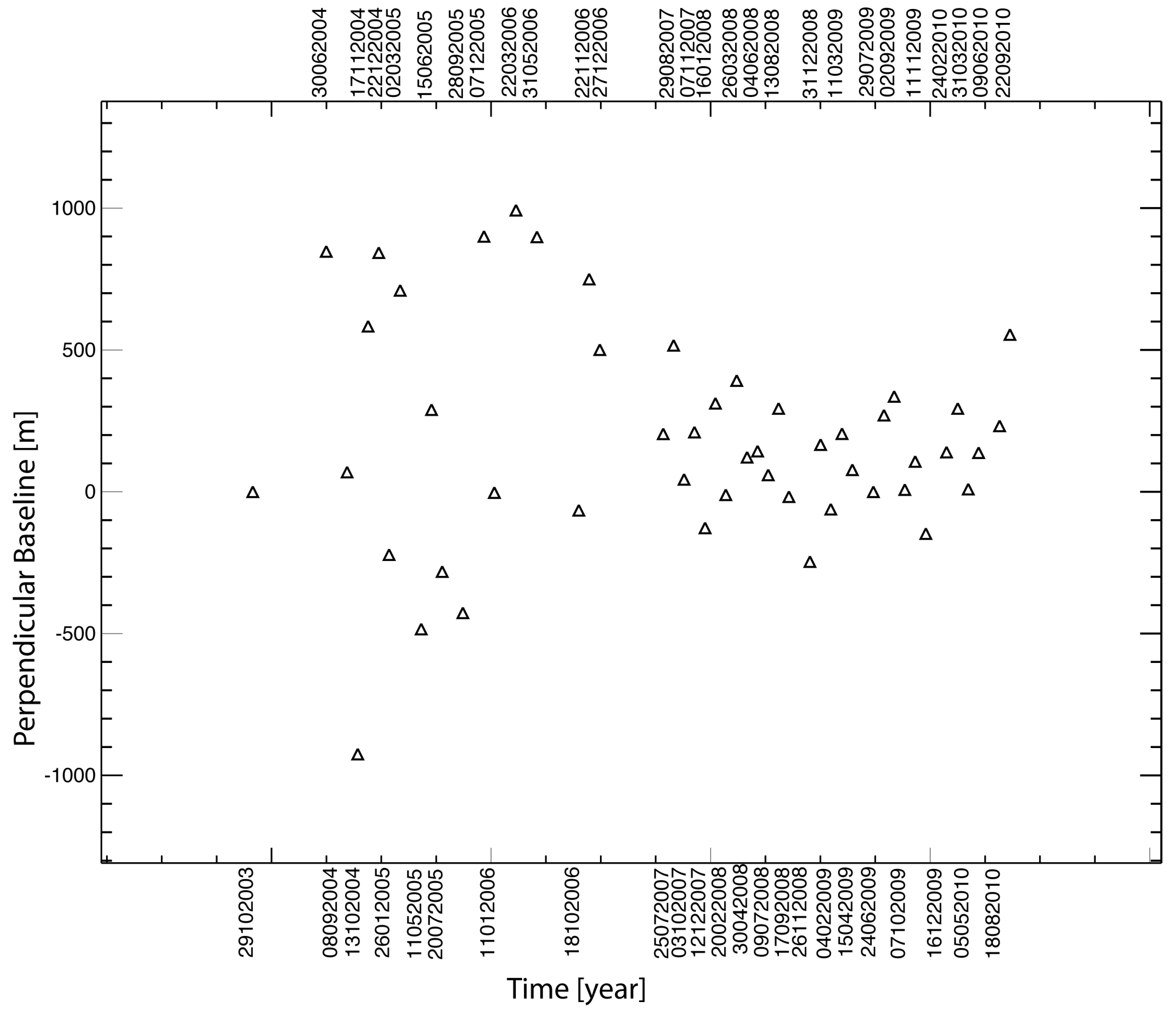
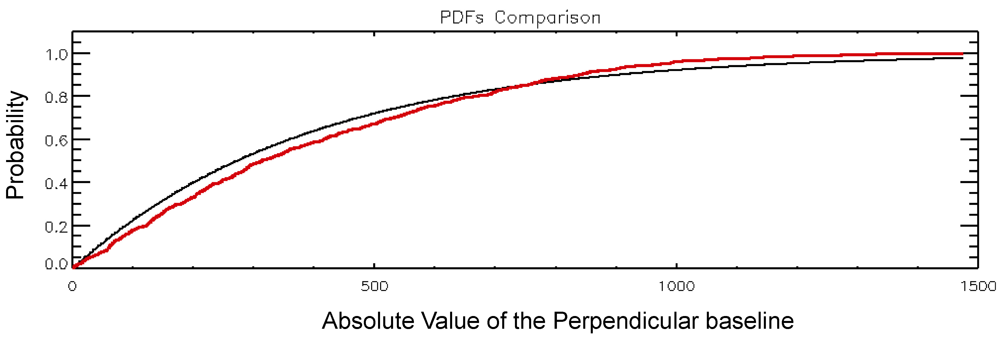
is the critical baseline. Therefore, the standard deviation of the circular variation strictly depends on the perpendicular baseline values of the InSAR interferograms used within the entire non-linear optimization procedure. This result is one of the main outcomes of this research paper. The selection of more coherent interferograms has a role in the robustness of the used phase estimator. To infer the role of the perpendicular baselines, in this research, I have assumed that the perpendicular baselines of the interferograms are distributed with an exponential pdf. The experimental results carried out on real SAR data set (see
Section 4) has demonstrated the suitability of this assumption. Under this hypothesis, the InSAR perpendicular baselines have the following pdf [
42]:
where
is the parameter of the exponential distribution [
40]. The average and the root mean square values of the absolute perpendicular baseline of the interferograms are
and
, respectively. By considering Equation (32), then, it is easy to calculate:
and
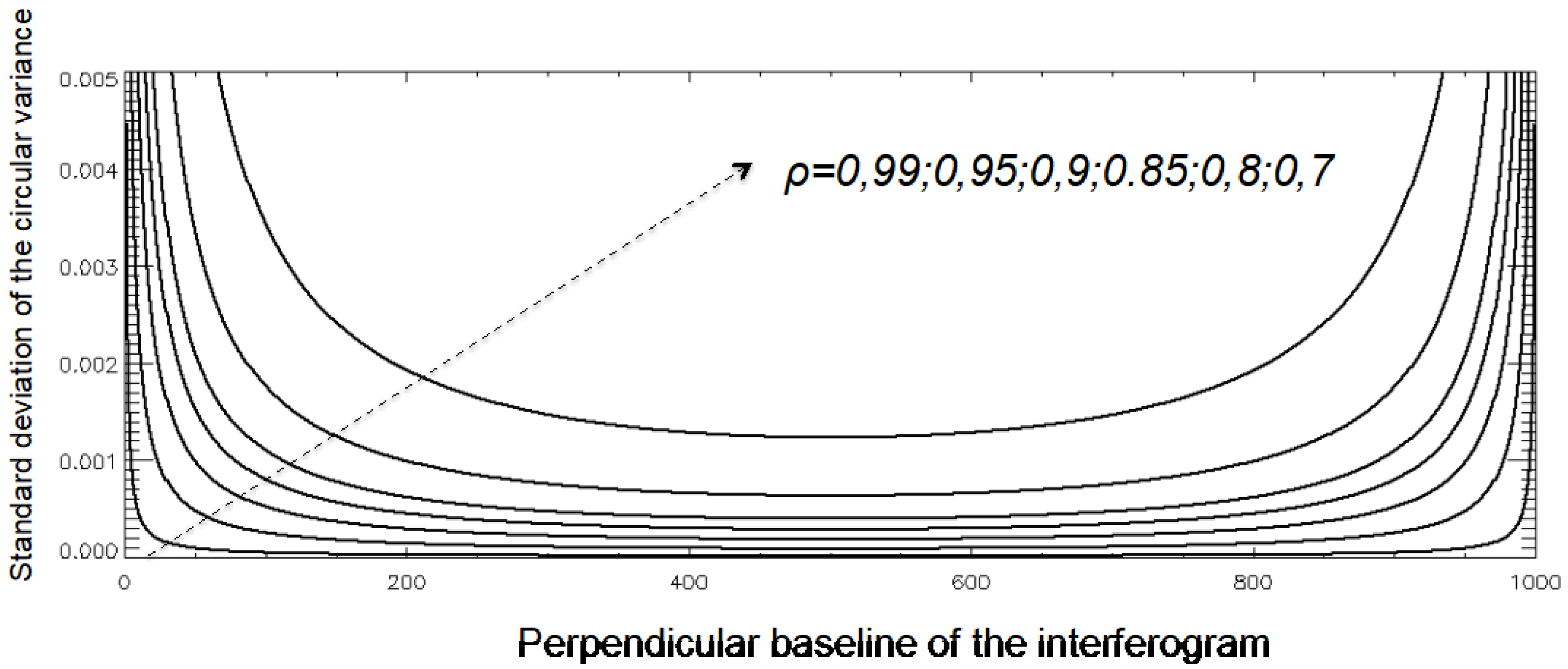
. By substitution in Equation (31):
Figure 4 plots the standard deviation of
versus the values of the average perpendicular baseline
for different values of
. In particular, I have assumed a critical baseline of 1000 m, a number of independent looks equal to L=30 and I considered M=1128 (see
Section 4) and
.
As evident, as the average perpendicular baseline λ approaches the critical baseline δb⊥c the standard deviation of the used estimator tends to diverge, as expected.
3.3. Theoretic Performance of the E-MTInSAR Noise Filtering Procedure
In this Subsection, I would like to give some introductory insights into the quality of the reconstructed interferograms. The obtained outcomes can be generally extended in other research fields, even very far from the one that is the subject of this research, where circular data (e.g., see [
43,
44,
45]) are used and the estimator of Equation (4) is employed. Of course, additional experiments and further studies are needed to have a closed-form solution for the problem of the statistical characterization of the retrievable noise-filtered interferograms and the relevant DInSAR deformation products: This is a matter for future investigations.
First of all, I would like to remark that the measured optimal mean resultant length, namely
, also gives an indirect estimate of the standard deviation of the residual phase, which was suitably assumed as independent and identically distributed. In particular, as earlier demonstrated: var[Θ] ≅ −2ln
ρ. However, the residual phases
take into account both the original
and the reconstructed interferograms. Accordingly, as a first approximation, if we initially assume that original
and reconstructed
interferograms are mutually independent, it can be argued that [
42]:
However, the original interferograms are not identically distributed and, as a consequence, the same happens for the reconstructed interferograms. In particular:
Under the hypothesis of independence, it is clear that the interferograms that were formerly with low spatial coherence and large standard deviations correspond to reconstructed interferograms with small standard deviations and higher coherence values, as also experimentally demonstrated in Reference [
26], and further corroborated by the experimental results shown in
Section 4. Of course, the hypothesis on the independence between the original and the reconstructed interferograms should be relaxed assuming there is a specific correlation between them (see the theory on InSAR noise models addressed in Reference [
42], for instance). More precisely, if we assume, for the sake of simplicity, that the original and reconstructed interferograms are jointly Gaussian with the correlation coefficient
η, we can then state that:
and the following relation holds:
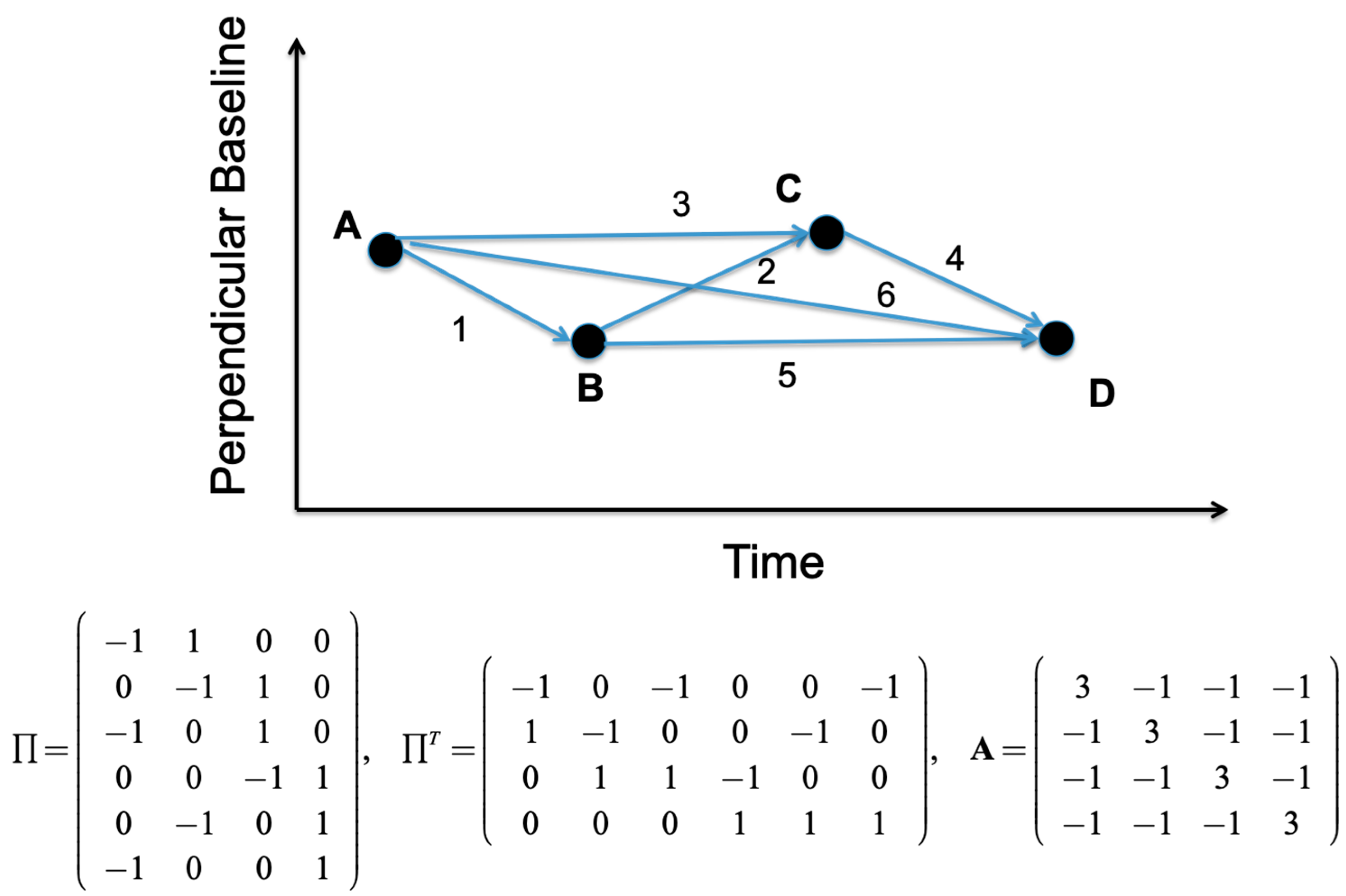
A more reliable estimate of the statistics of the reconstructed interferograms would require the knowledge of the incidence matrix ∏ of the oriented graph
G representing the InSAR data distribution, which specifies the edge-node connectivity relations among the network of interferograms into the temporal/perpendicular baseline plane. Therein, the nodes of the graph identify the used SAR data and the edges the selected interferometric SAR data pairs. As an example, see the picture depicted in
Figure 5, where a possible distribution of four nodes and six edges is simulated.
To infer the standard deviation of the reconstructed interferograms, the minimization of the circular variance in Equation (12) represents, again, the starting point.
As said, the optimal phase estimates related to the available SAR acquisitions are those that minimize the following mathematical operator:
In correspondence to the stationary phase point, the following relations hold:
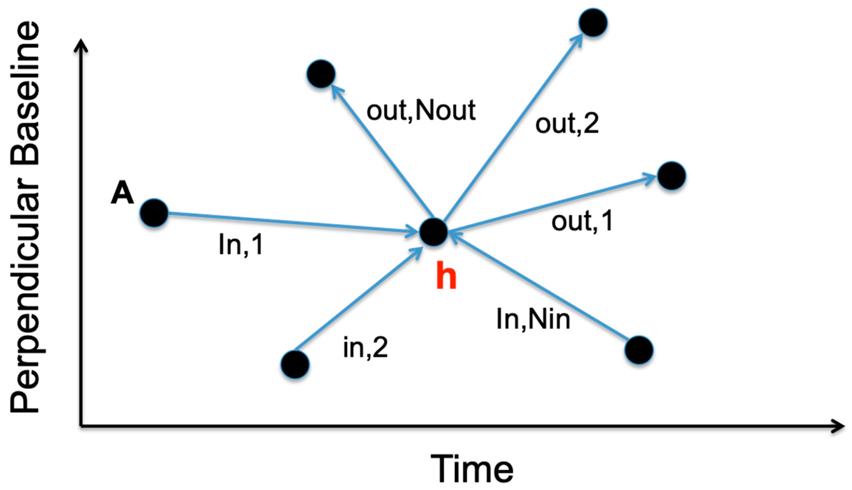
The derivative terms that are present in Equation (40) can assume values –1,0,1 depending on the fact that the
h-node of the oriented graph
G, see for instance the example shown in
Figure 6, is involved in the
i-th InSAR data pair (an edge of the graph G). In particular:
If we indicate with the number of edges that exit from the node h and with the number of edges that enter the node h, it is pretty easy to demonstrate that condition (40) is equivalent to:
Equation (42) can also be re-organized as follows:
Using matrix formalism, Equation (43) can simply be written as:
By inspecting Equation (43) and using discrete calculus principles and graph theory [
46], it can be easily shown that the matrixes
and
can be expressed as follows:
where
is the vector (Mx1) of the weights used during the optimization procedure, and the symbol∘ stands for the Hadamard product.
Figure 6 shows the expression of
A and
B matrices for the simplified graph depicted in
Figure 6. It is worth noting that if the weights are all unitary, the matrix
represents the discrete Laplacian matrix [
46] of the graph G; thus
. The matrix
has several interesting properties and is mostly used in the research field of spectral clustering [
46,
47]. Here, I will only mention the properties that are significant for the present research work.
The graph Laplacian matrix of a graph is defined as:
where
and
are the degree matrix and the adjacency matrix of the network, respectively, see [
46] for details. More importantly, the matrix
is: (i) Symmetric and positive semi-definite, (ii) its smallest eigenvalues is zero, and the corresponding eigenvector is the constant one vector; (iii) it has all real-valued eigenvalues. Because at least one of the eigenvalues is equal to zero, the Laplacian matrix is not invertible. However, a generalized inverse is defined using the following matrix decomposition:
where
is the matrix containing all eigenvectors as columns and Λ
+ is the diagonal matrix with the eigenvalues on its diagonal. Interested readers can find further details on the inverse of the Laplacian graph matrix in [
47]. Another example, for a simple triangular oriented grid, is shown in
Figure 7. I would also like to point out that, in the simplified case that all the weights are unitary, the following relation holds:
where the properties of the wrapping operator have been used. Indeed, the relation in Equation (44) involves (wrapped) phase terms but matrix multiplication can be only performed on absolute (unwrapped) phase quantities. However, this does not represent a severe drawback, at least when the weights are unitary, because wrapped and unwrapped phases differ by multiple-integer matrixes of
. Accordingly, by using Equation (44), the expression (48) is valid.
Analysis of Equation (48) evidences another essential result of this research paper: When the phase noise vector term is not present, i.e., when the original interferograms are fully time-consistent, the reconstructed and the original interferograms are necessarily the same. This outcome is not surprising, and it demonstrates that the condition expressed by Equation (3) is required for the application of the developed noise-filtering method.
Generally speaking, the condition (see Equation (48)):
means that, under the hypothesis that original interferograms are uncorrelated, the (wrapped) discrete divergence of the reconstructed interferograms, namely
, equals the (wrapped) divergence of the original interferograms, namely
.
Equation (45) and the property (49) of the reconstructed interferograms may be exploited to calculate the covariance matrix of the reconstructed interferograms. In particular, for the sake of simplicity, let us refer to the (unwrapped) quantities. In this case, assuming that all weights are unitary, the covariance matrix of the optimal phase vector related to the SAR acquisition is related to the covariance matrix of the original interferograms as expressed below:
Finally, if we assume that original interferograms were all uncorrelated, independent and identically distributed with standard deviation
, the co-variance matrix of the reconstructed phases related to each SAR acquisition, see Equation (50), is as follows:
The outcome expressed by Equations (50) and (51) is significant, even it is not definitive. This research paper represents a step forward to Reference [
26]. Additional efforts are required to extend the result of Equation (51) in a broader context, with the aim to identify how to select and use the original interferograms to maximize the performance of the E-MTInSAR noise-filtering technique. In this framework, the role of the weights in Equation (45) has to be taken into account for future analyses.


