Application of a Small Baseline Subset Time Series Method with Atmospheric Correction in Monitoring Results of Mining Activity on Ground Surface and in Detecting Induced Seismic Events


Abstract
:
1. Introduction
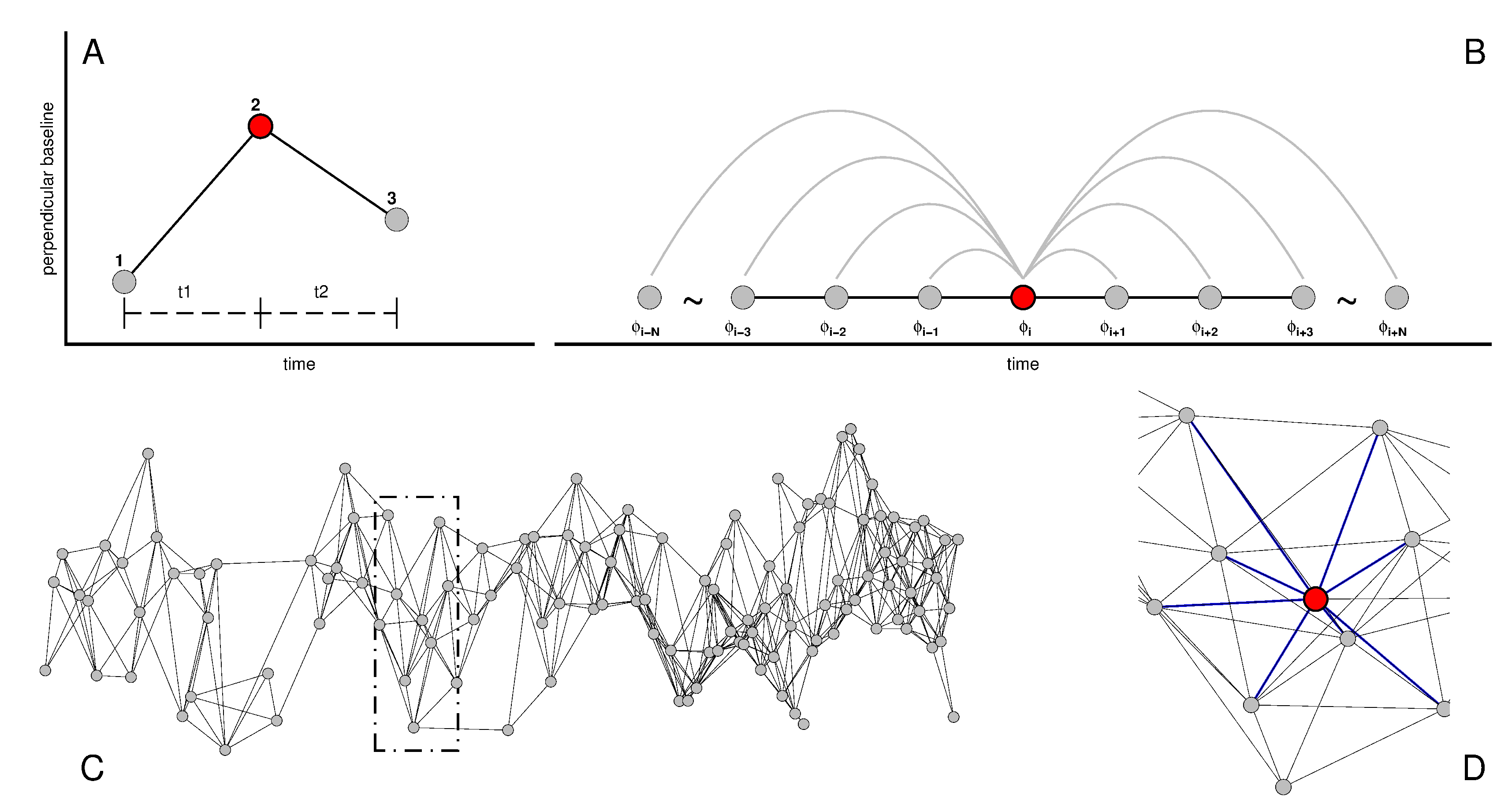
2. Methods
3. Area of Study
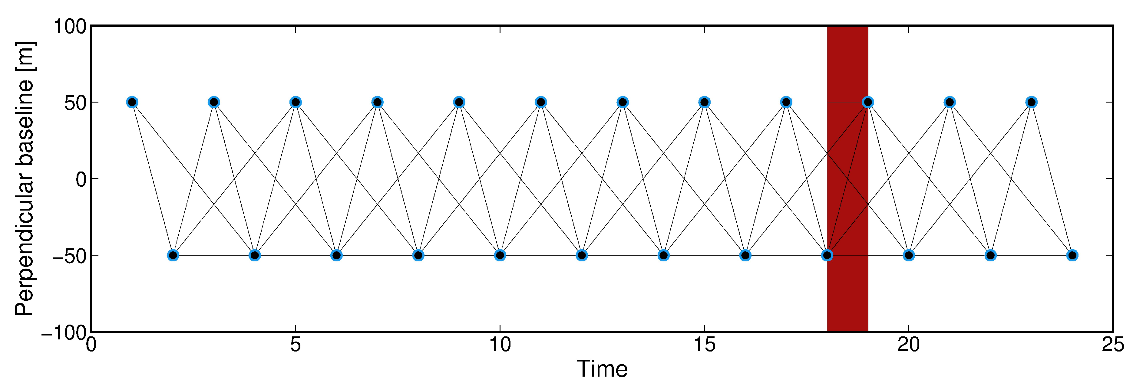
4. Data Time Series Processing
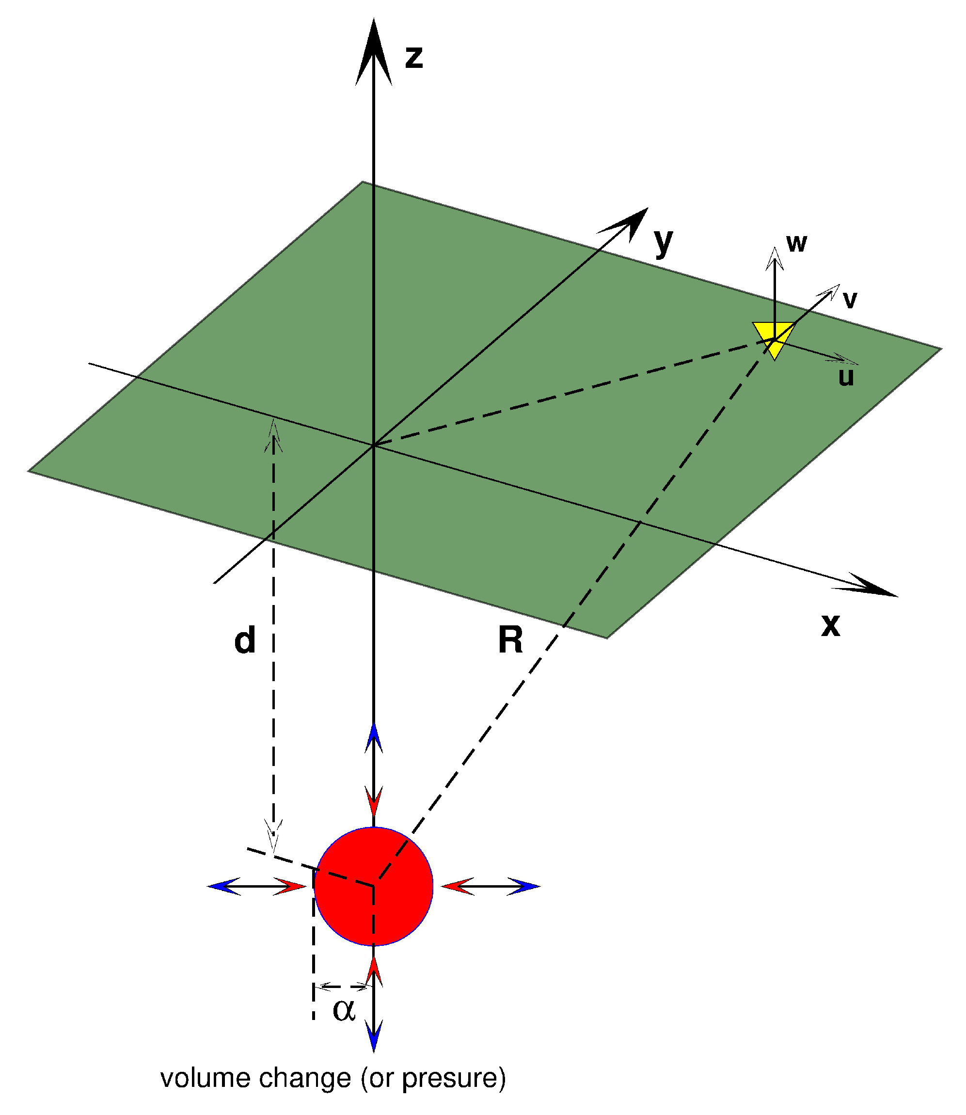
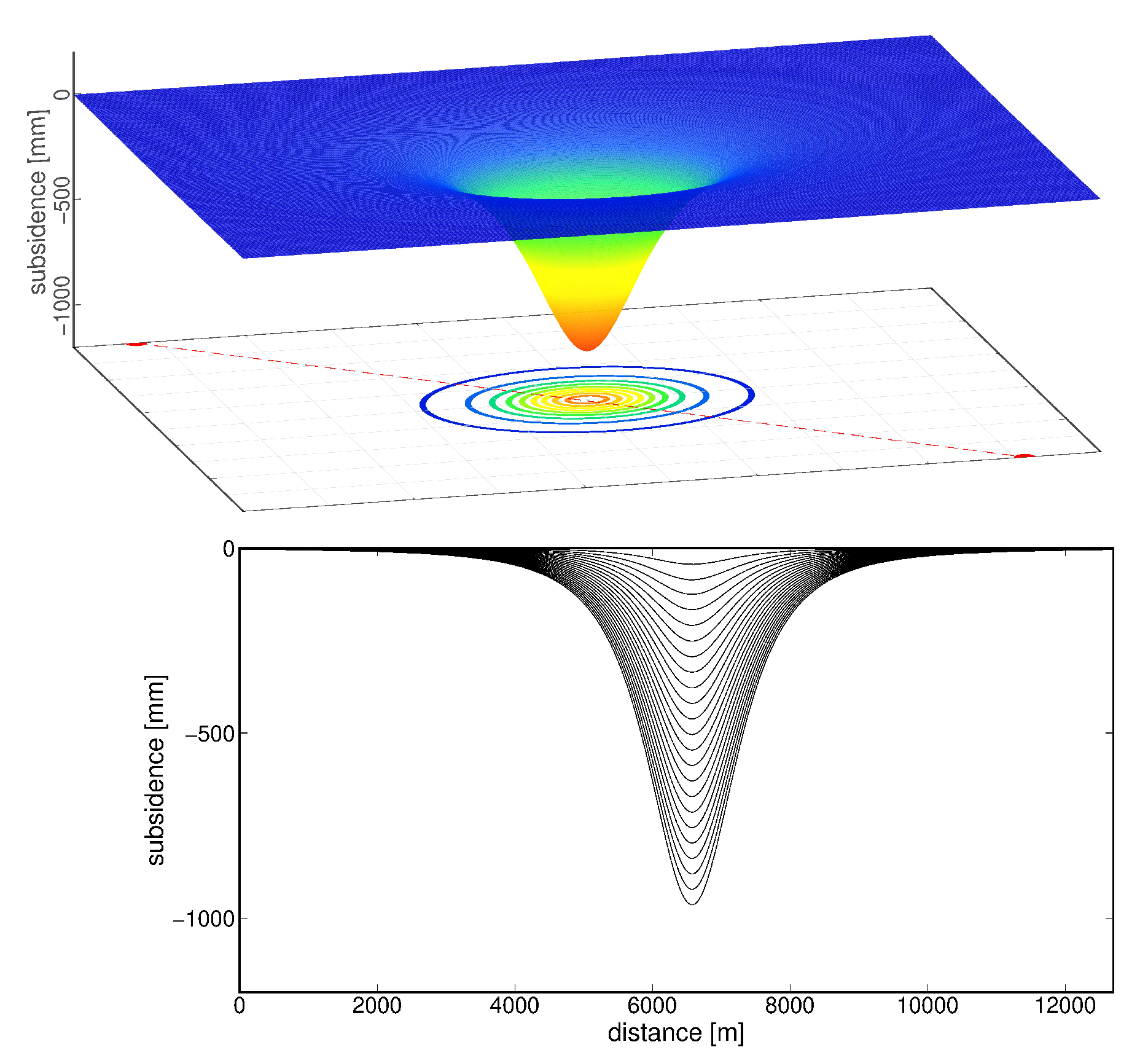
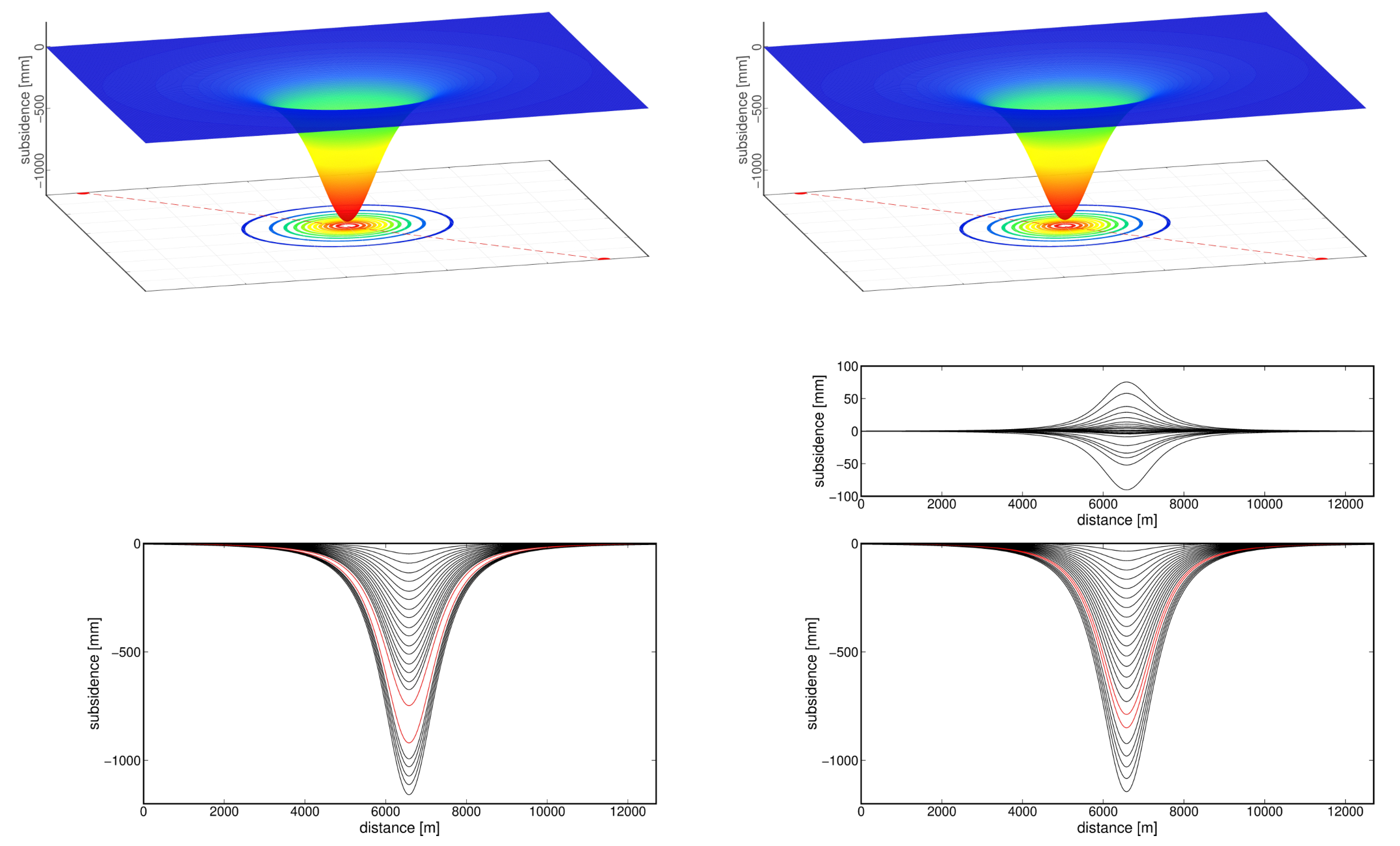
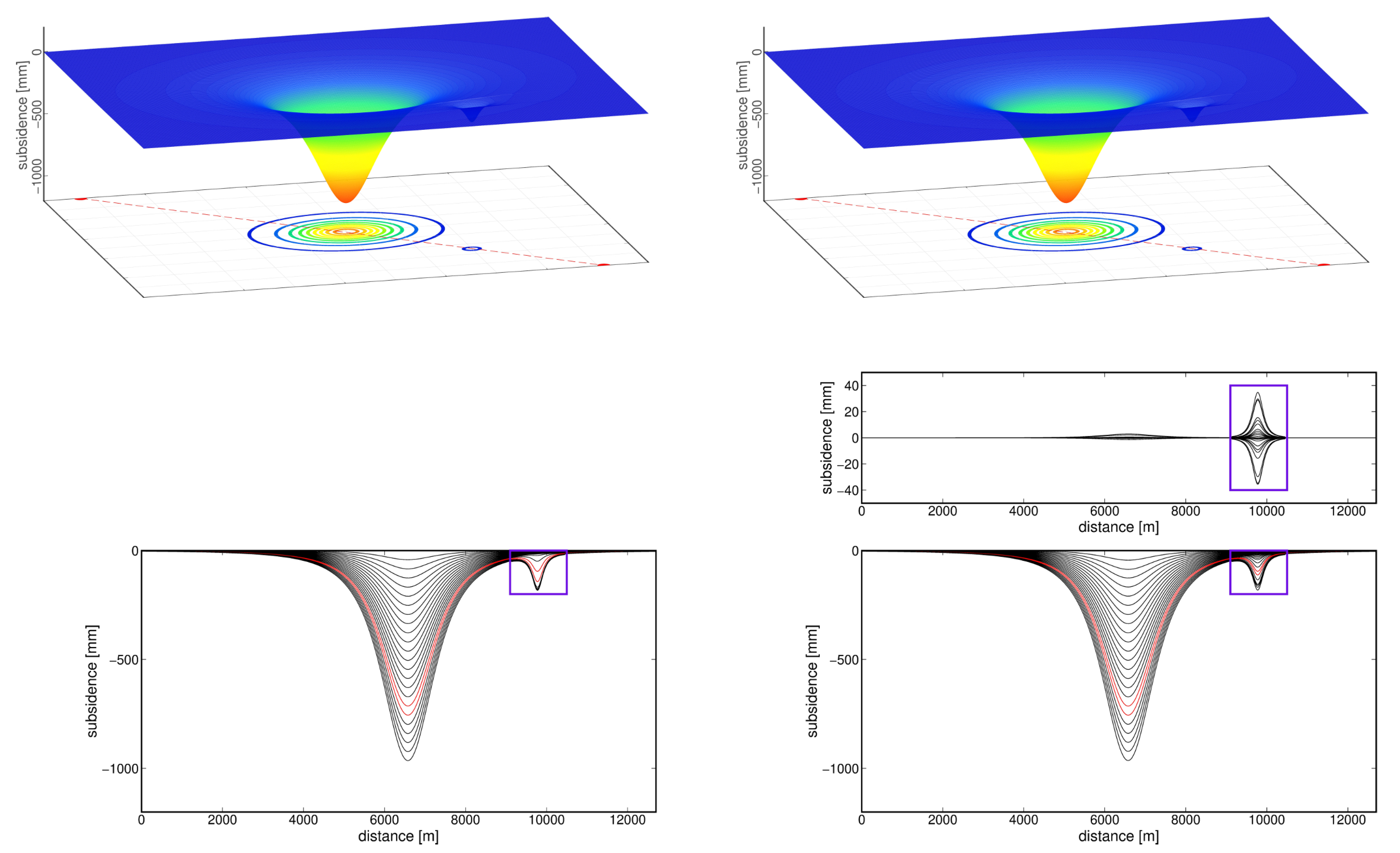
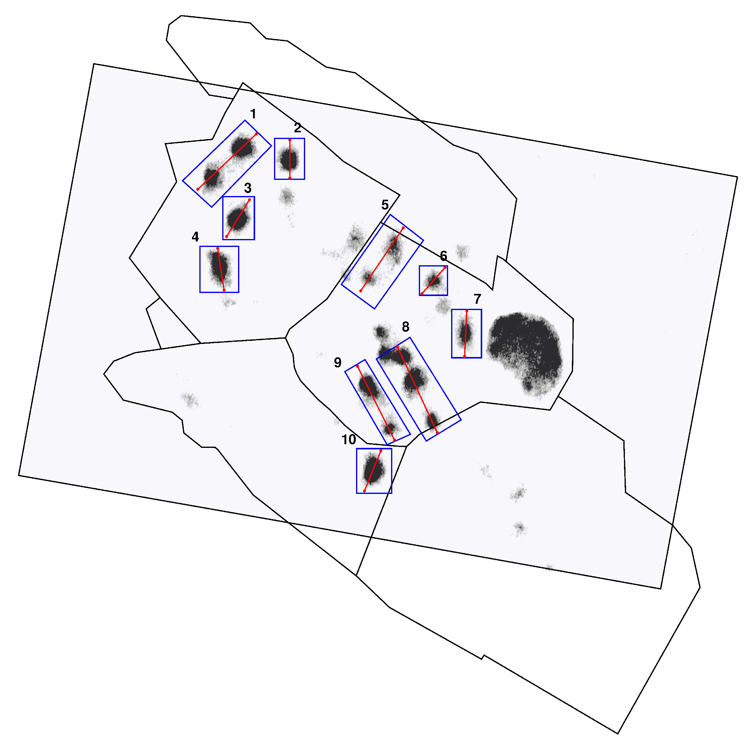
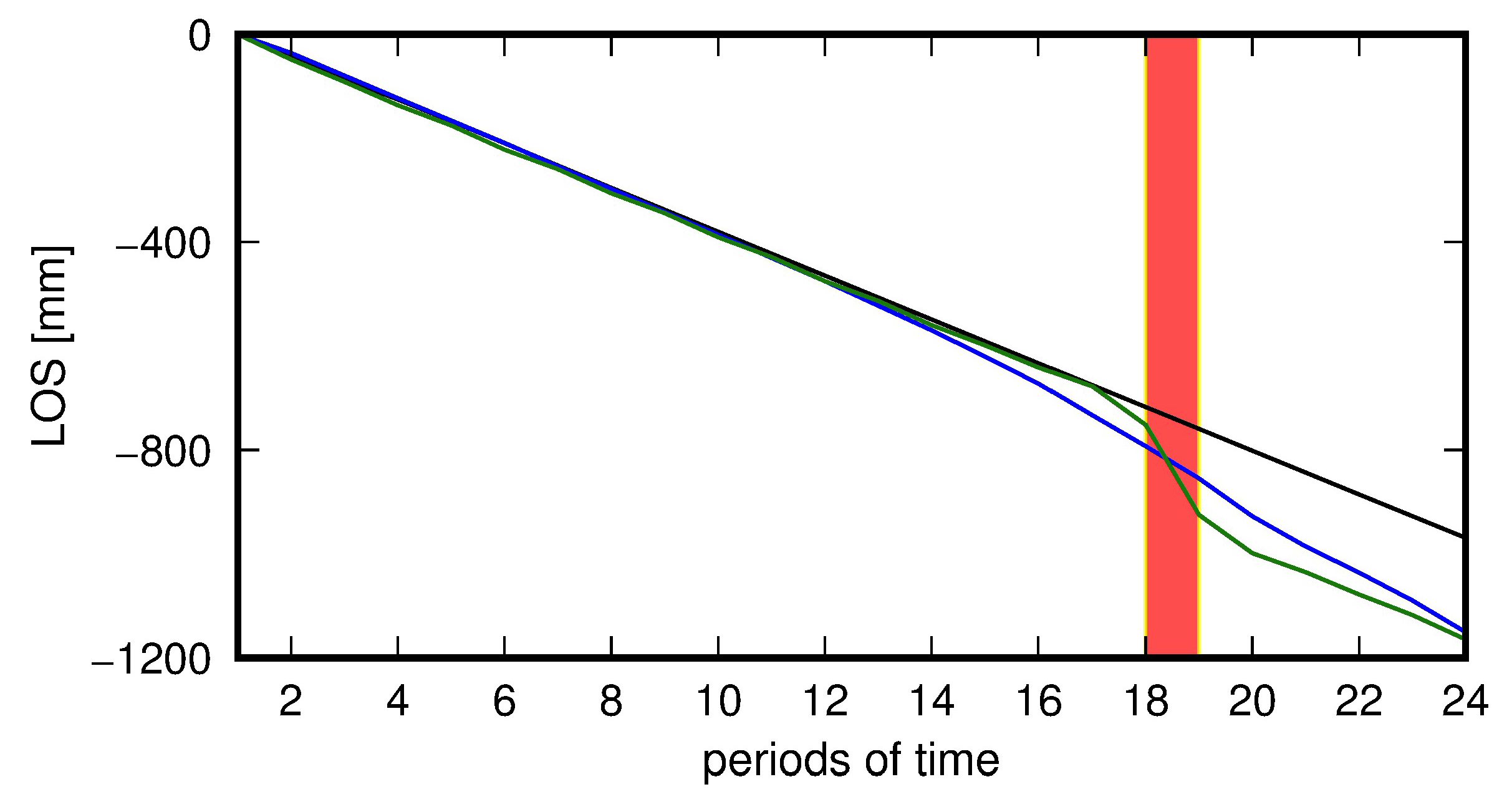
4.1. Test Calculations: Application of the Mogi Model
- (I)
- mining activity without a mining tremor,
- (II)
- mining activity with a mining tremor recorded between and , the tremor having occurred exactly in the center of the already existing subsidence trough,
- (III)
- mining activity with a mining tremor recorded between and , but unlike in case (II) the tremor occurred outside the mining area influenced by mining operations and was located at a distance of approximately 3 km from the center of the already existing subsidence trough.
4.2. Calculations for the Lgcb Region
5. Results
5.1. Test Calculations—Application of the Mogi Model
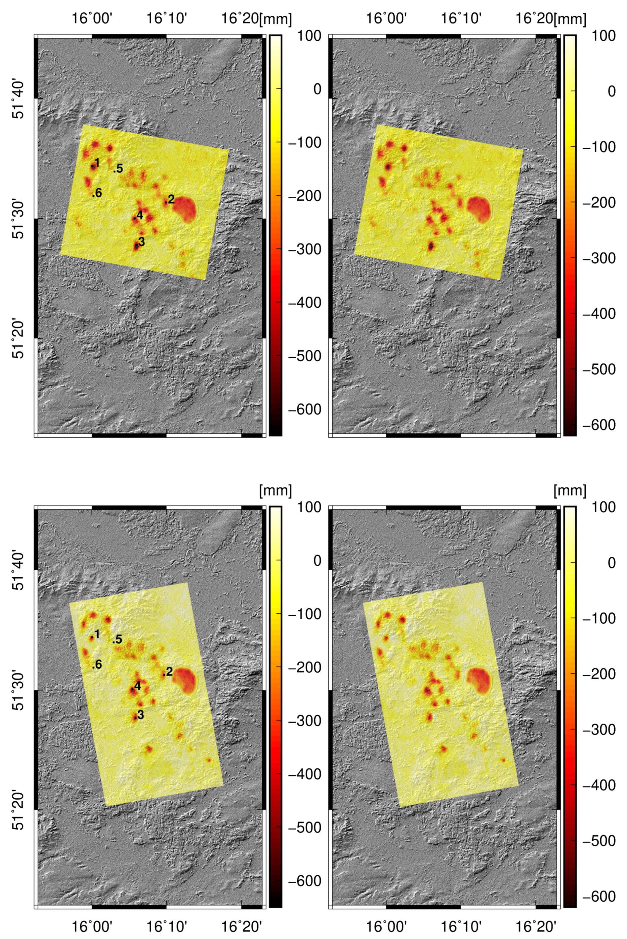
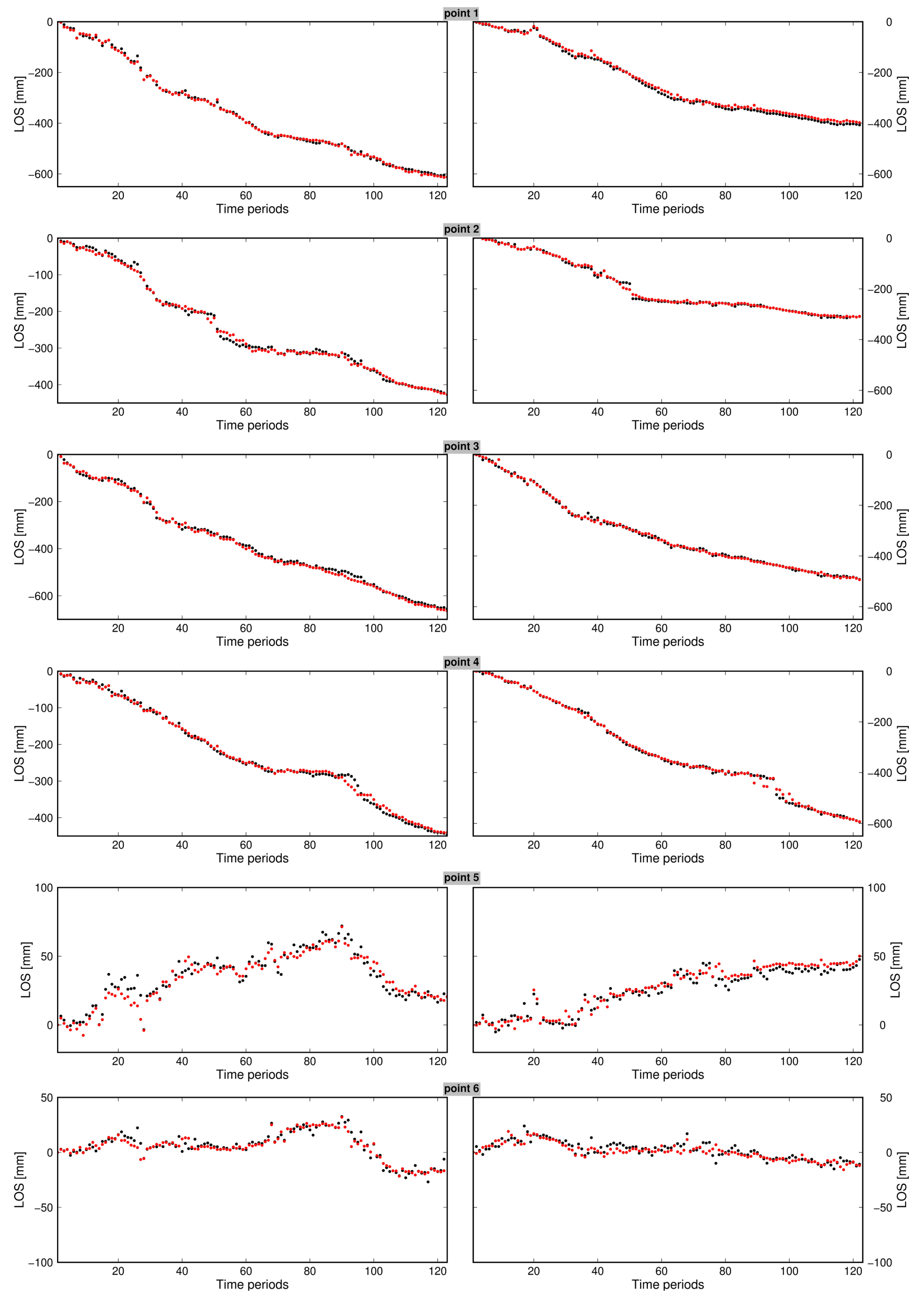
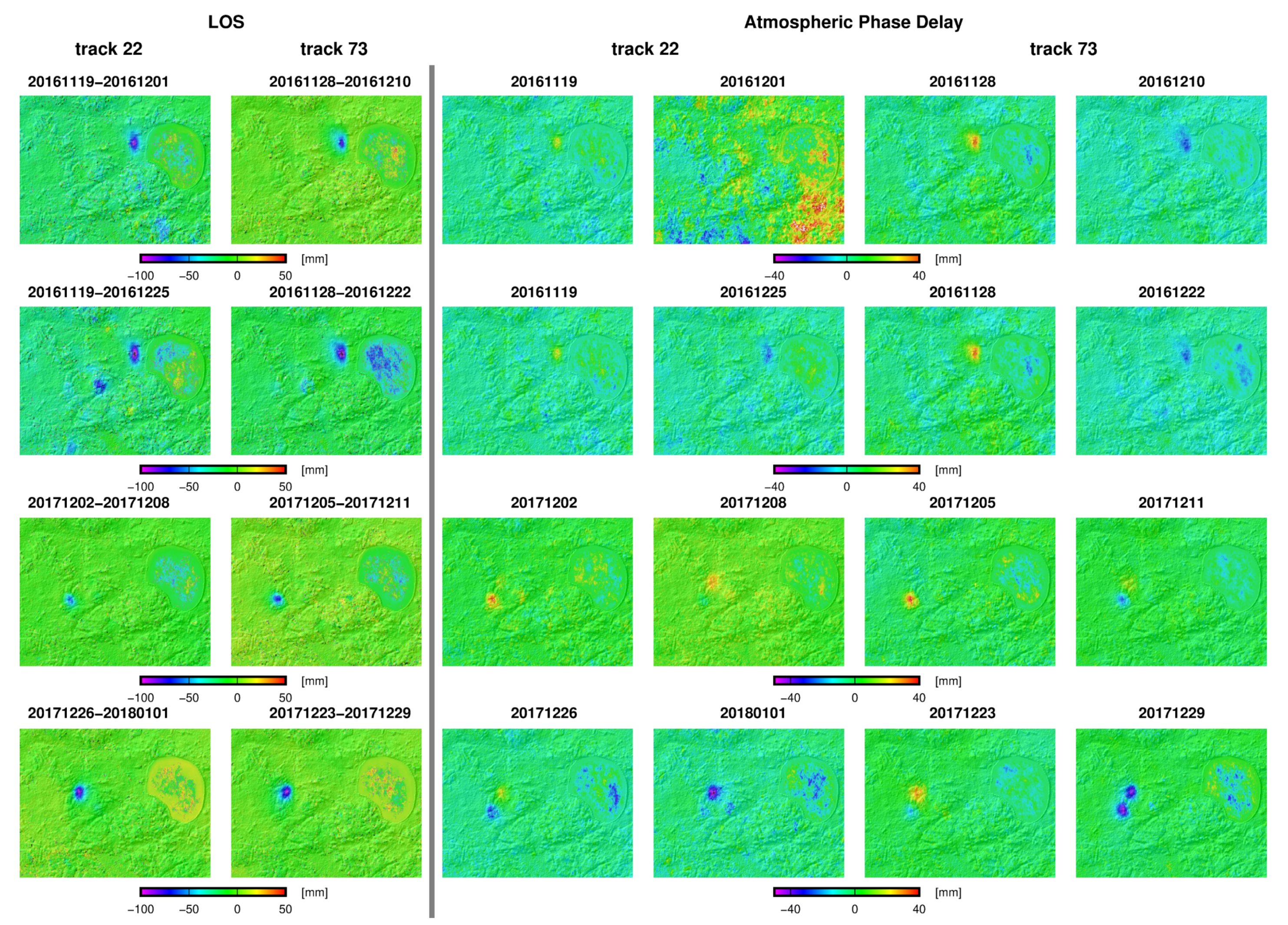
5.2. Calculations for the Lgcb Region
6. Discussion
7. Conclusions
Funding
Conflicts of Interest
References
- Brady, B.H.G.; Brown, E.T. Rock Mechanics, 3rd ed.; Chapter 16; Springer: Dordrecht, The Netherlands, 2006; p. 628. [Google Scholar]
- Samsonov, S.; Smets, B.; D’Oreye, N.; Smets, B. Ground deformation associated with post-mining activity at the French—German border revealed by novel InSAR time series method. Int. J. Appl. Earth Obs. Geoinf. 2013, 23, 142–154. [Google Scholar] [CrossRef]
- Szczerbowski, Z.; Jura, J. Mining induced seismic events and surface deformations monitored by GPS permanent stations. Acta Geodyn. Et Geomater. 2015, 12, 237–248. [Google Scholar] [CrossRef]
- Doležalová, H.; Kajzar, V.; Souček, K.; Staš, L. Evaluation of mining subsidence using GPS data. Acta Geodyn. Et Geomater. 2009, 6, 359–367. [Google Scholar]
- Yue, D.; Wang, J.; Zhou, J.; Chen, X.; Ren, H. Monitoring slope deformation using a 3-D laser image scanning system: A case study. Min. Sci. Technol. 2010, 20, 898–903. [Google Scholar] [CrossRef]
- Xu, Z.; Xu, E.; Wu, L.; Liu, S.; Mao, Y. Registration of Terrestrial Laser Scanning Surveys Using Terrain-Invariant Regions for Measuring Exploitative Volumes over Open-Pit Mines. Remote Sens. 2019, 11, 606. [Google Scholar] [CrossRef]
- Antonello, G.; Casagli, N.; Farina, P.; Leva, D.; Nico, G.; Sieber, A.J.; Tarchi, D. Ground-based SAR interferometry for monitoring mass movements. Landslides 2004, 1, 21–28. [Google Scholar] [CrossRef]
- Carlà, T.; Farina, P.; Intrieri, E.; Ketizmen, H.; Casagli, N. Integration of ground-based radar and satellite InSAR data for the analysis of an unexpected slope failure in an open-pit mine. Eng. Geol. 2018, 235, 39–52. [Google Scholar] [CrossRef]
- Duque, S.; Lopez-Sanchez, J.; Mallorqui, J.; Herrera, G.; Tomás, R.; Mulas, J.; Delgado, J. Advanced DInSAR analysis on mining areas: La Union case study (Murcia, SE Spain). Eng. Geol. 2007, 90, 148–159. [Google Scholar] [Green Version]
- Paradella, W.R.; Ferretti, A.; Mura, J.C.; Colombo, D.; Gama, F.F.; Tamburini, A.; Santos, A.R.; Novali, F.; Galo, M.; Camargo, P.O.; et al. Mapping surface deformation in open pit iron mines of Carajás Province (Amazon Region) using an integrated SAR analysis. Eng. Geol. 2015, 193, 61–78. [Google Scholar] [CrossRef] [Green Version]
- Peduto, D.; Nicodemo, G.; Maccabiani, J.; Ferlisi, S. Multi-scale analysis of settlement-induced building damage using damage surveys and DInSAR data: A case study in The Netherlands. Eng. Geol. 2017, 218, 117–133. [Google Scholar] [CrossRef]
- Jung, H.C.; Kim, S.W.; Jung, H.S.; Min, K.D.; Won, J.S. Satellite observation of coal mining subsidence by persistent scatterer analysis. Eng. Geol. 2007, 92, 1–13. [Google Scholar] [CrossRef]
- Liu, D.; Shao, Y.; Liu, Z.; Riedel, B.; Sowter, A.; Niemeier, W.; Bian, Z. Evaluation of InSAR and TomoSAR for Monitoring Deformations Caused by Mining in a Mountainous Area with High Resolution Satellite-Based SAR. Remote Sens. 2014, 6, 1476–1495. [Google Scholar] [CrossRef] [Green Version]
- Ma, C.; Cheng, X.; Yang, Y.; Zhang, X.; Guo, Z.; Zou, Y. Investigation on Mining Subsidence Based on Multi-Temporal InSAR and Time-Series Analysis of the Small Baseline Subset—Case Study of Working Faces 22201-1/2 in Bu’ertai Mine, Shendong Coalfield, China. Remote Sens. 2016, 8. [Google Scholar] [CrossRef]
- Zhao, C.; Lu, Z.; Zhang, Q. Time-series deformation monitoring over mining regions with SAR intensity-based offset measurements. Remote Sens. Lett. 2013, 4, 436–445. [Google Scholar] [CrossRef]
- Cuenca, C.M.; Hooper, A.J.; Hanssen, R.F. Surface deformation induced by water influx in the abandoned coal mines in Limburg, The Netherlands observed by satellite radar interferometry. J. Appl. Geophys. 2013, 88, 1–11. [Google Scholar] [CrossRef]
- Milczarek, W.; Blachowski, J.; Grzempowski, P. Application of PSInSAR for assessment of surface deformations in post-mining area—Case study of the former Walbrzych hard coal basin (SW Poland). Acta Geodyn. Et Geomater. 2017, 14, 41–52. [Google Scholar]
- Popiolek, E.; Ostrowski, J.; Czaja, J.; Mazur, J. Poster_Paper 9.pdf. In Proceedings of the 10th FIG International Symposium on Deformation Measurements, International Federation of Surveyors, Orange, CA, USA, 19–21 March 2001; pp. 77–80. [Google Scholar]
- Tymofyeyeva, E.; Fialko, Y. Mitigation of atmospheric phase delays in InSAR data, with application to the eastern California shear zone. J. Geophys. Res. Solid Earth 2015, 120, 5952–5963. [Google Scholar] [CrossRef] [Green Version]
- Bürgmann, R.; Rosen, P.A.; Fielding, E.J. Synthetic Aperture Radar Interferometry to Measure Earth’s Surface Topography and Its Deformation. Annu. Rev. Earth Planet. Sci. 2000, 28, 169–209. [Google Scholar] [CrossRef]
- Brcic, R.; Parizzi, A.; Eineder, M.; Bamler, R.; Meyer, F. Estimation and compensation of ionospheric delay for SAR interferometry. Int. Geosci. Remote Sens. Symp. 2010, 2908–2911. [Google Scholar] [CrossRef]
- Yu, C.; Li, Z.; Penna, N.T.; Crippa, P. Generic Atmospheric Correction Model for Interferometric Synthetic Aperture Radar Observations. J. Geophys. Res. Solid Earth 2018, 9202–9222. [Google Scholar] [CrossRef]
- Bekaert, D.P.S.; Walters, R.J.; Wright, T.J.; Hooper, A.J.; Parker, D.J. Statistical comparison of {InSAR} tropospheric correction techniques. Remote Sens. Environ. 2015, 170, 40–47. [Google Scholar] [CrossRef]
- Xu, X.; Sandwell, D.T.; Tymofyeyeva, E.; González-Ortega, A.; Tong, X. Tectonic and {Anthropogenic} {Deformation} at the {Cerro} {Prieto} {Geothermal} {Step}-{Over} {Revealed} by {Sentinel}-1A {InSAR}. IEEE Trans. Geosci. Remote Sens. 2017, 55, 5284–5292. [Google Scholar] [CrossRef]
- Mogi, K. Relations between the eruptions of various volcanoes and the deformations of the ground surfaces around them. Bull. Earthq. Res. Inst 1958, 36, 99–134. [Google Scholar]
- Meo, M.; Tammaro, U.; Capuano, P. Influence of topography on ground deformation at Mt. Vesuvius (Italy) by finite element modelling. Int. J. Non-Linear Mech. 2008, 43, 178–186. [Google Scholar] [CrossRef] [Green Version]
- Masterlark, T. Magma intrusion and deformation predictions: Sensitivities to the Mogi assumptions. J. Geophys. Res. Solid Earth 2007, 112, 1–17. [Google Scholar] [CrossRef]
- Freymueller, J.T.; Kaufman, A.M. Changes in the magma system during the 2008 eruption of Okmok volcano, Alaska, based on GPS measurements. J. Geophys. Res. Solid Earth 2010, 115, 1–14. [Google Scholar] [CrossRef]
- Fuhrmann, T.; Garthwaite, M.C. Resolving Three-Dimensional Surface Motion with InSAR: Constraints from Multi-Geometry Data Fusion. Remote Sens. 2019, 11, 241. [Google Scholar] [CrossRef]
- Berardino, P.; Fornaro, G.; Lanari, R.; Sansosti, E. A new algorithm for surface deformation monitoring based on small baseline differential {SAR} interferograms. IEEE Trans. Geosci. Remote Sens. 2002, 40, 2375–2383. [Google Scholar] [CrossRef]
- Lanari, R.; Mora, O.; Manunta, M.; Mallorqui, J.J.; Berardino, P.; Sansosti, E. A small-baseline approach for investigating deformations on full-resolution differential SAR interferograms. IEEE Trans. Geosci. Remote Sens. 2004, 42, 1377–1386. [Google Scholar] [CrossRef]
- Lanari, R.; Casu, F.; Manzo, M.; Zeni, G.; Berardino, P.; Manunta, M.; Pepe, A. An Overview of the Small BAseline Subset Algorithm: A DInSAR Technique for Surface Deformation Analysis. In Deformation and Gravity Change: Indicators of Isostasy, Tectonics, Volcanism, and Climate Change; Wolf, D., Fernández, J., Eds.; Birkhäuser Basel: Basel, Switzerland, 2007; pp. 637–661. [Google Scholar]
- Orlecka-Sikora, B.; Papadimitriou, E.E.; Kwiatek, G. A study of the interaction among mining-induced seismic events in the Legnica-Głogów Copper District, Poland. Acta Geophys. 2009, 57, 413–434. [Google Scholar] [CrossRef] [Green Version]
- Gibowicz, S.J. Seismic doublets and multiplets at Polish coal and copper mines. Acta Geophys. 2006, 54, 142–157. [Google Scholar] [CrossRef]
- Trenczek, S. Study of influence of tremors on combined hazards. Longwall mining operations in co-occurrence of natural hazards. A case study. J. Sustain. Min. 2016, 15, 36–47. [Google Scholar] [CrossRef] [Green Version]
- Gibowicz, S.; Kijko, A. An Introduction to Mining Seismology; Academic Press: New York, NY, USA, 1994; chapter 2; pp. 15–23. [Google Scholar]
- Drzewiecki, J.; Piernikarczyk, A. The forecast of mining-induced seismicity and the consequent risk of damage to the excavation in the area of seismic event. J. Sustain. Min. 2017, 16, 1–7. [Google Scholar] [CrossRef]
- Kubacki, T.; Koper, K.D.; Pankow, K.L.; McCarter, M.K. Changes in mining-induced seismicity before and after the 2007 Crandall Canyon Mine collapse. J. Geophys. Res. Solid Earth 2014, 119, 4876–4889. [Google Scholar] [CrossRef] [Green Version]
- Krawczyk, A.; Grzybek, R. An evaluation of processing InSAR Sentinel-1A/B data for correlation of mining subsidence with mining induced tremors in the Upper Silesian Coal Basin (Poland). E3S Web Conf. 2018, 26, 1–5. [Google Scholar] [CrossRef]
- Bommer, J.J.; Crowley, H.; Pinho, R. A risk-mitigation approach to the management of induced seismicity. J. Seismol. 2015, 19, 623–646. [Google Scholar] [CrossRef] [Green Version]
- Lei, X.; Huang, D.; Su, J.; Jiang, G.; Wang, X.; Wang, H.; Guo, X.; Fu, H. Fault reactivation and earthquakes with magnitudes of up to Mw4.7 induced by shale-gas hydraulic fracturing in Sichuan Basin, China. Sci. Rep. 2017, 7, 1–12. [Google Scholar] [CrossRef]
- Corlett, H.; Schultz, R.; Branscombe, P.; Hauck, T.; Haug, K.; MacCormack, K.; Shipman, T. Subsurface faults inferred from reflection seismic, earthquakes, and sedimentological relationships: Implications for induced seismicity in Alberta, Canada. Mar. Pet. Geol. 2018, 93, 135–144. [Google Scholar] [CrossRef]
- Barnhart, W.D.; Benz, H.M.; Hayes, G.P.; Rubinstein, J.L.; Bergman, E.; Benz, H.M.; Hayes, G.P.; Rubinstein, J.L.; Bergman, E. Seismological and geodetic constraints on the 2011 Mw5. 3 Trinidad, Colorado earthquake and induced deformation in the Raton Basin. J. Geophys. Res. Solid Earth 2014, 119, 7923–7933. [Google Scholar] [CrossRef]
- Vlek, C. Induced Earthquakes from Long-Term Gas Extraction in Groningen, the Netherlands: Statistical Analysis and Prognosis for Acceptable-Risk Regulation. Risk Anal. 2018, 38, 1455–1473. [Google Scholar] [CrossRef] [PubMed] [Green Version]
- Diehl, T.; Kraft, T.; Kissling, E.; Wiemer, S. The induced earthquake sequence related to the St. Gallen deep geothermal project (Switzerland): Fault reactivation and fluid interactions imaged by microseismicity. J. Geophys. Res. Solid Earth 2017, 122, 7272–7290. [Google Scholar] [CrossRef]
- van der Baan, M.; Calixto, F.J. Human-induced seismicity and large-scale hydrocarbon production in the USA and Canada. Geochem. Geophys. Geosyst. 2017, 116, 1–12. [Google Scholar] [CrossRef]
- Did anthropogenic activities trigger the 3 April 2017 Mw 6.5 Botswana earthquake? Remote Sens. 2017, 9, 1–12.
- White, J.A.; Foxall, W. Assessing induced seismicity risk at CO2 storage projects: Recent progress and remaining challenges. Int. J. Greenh. Gas Control 2016, 49, 413–424. [Google Scholar] [CrossRef]
- Verdon, J.P.; Stork, A.L. Carbon capture and storage, geomechanics and induced seismic activity. J. Rock Mech. Geotech. Eng. 2016, 8, 928–935. [Google Scholar] [CrossRef] [Green Version]
- Brodsky, E.E.; Lajoie, L.J. at the Salton Sea Geothermal Field. Science 2013, 543, 543–546. [Google Scholar] [CrossRef]
- Lin, G.; Wu, B. Seismic velocity structure and characteristics of induced seismicity at the Geysers Geothermal Field, eastern California. Geothermics 2018, 71, 225–233. [Google Scholar] [CrossRef]
- Fialko, Y.; Simons, M. Deformation and seismicity in the Coso geothermal area, Inyo County, California: Observations and modeling using satellite radar interferometry. J. Geophys. Res. Solid Earth 2000, 105, 21781–21793. [Google Scholar] [CrossRef] [Green Version]
- Vasco, D.W.; Rutqvist, J.; Ferretti, A.; Rucci, A.; Bellotti, F.; Dobson, P.; Oldenburg, C.; Garcia, J.; Walters, M.; Hartline, C. Monitoring deformation at the Geysers geothermal field, California using C-band and X-band interferometric synthetic aperture radar. Geophys. Res. Lett. 2013, 40, 2567–2572. [Google Scholar] [CrossRef]
- Weingarten, M.; Ge, S.; Godt, J.W.; Bekins, B.A.; Rubinstein, J.L. High-rate injection is associated with the increase in U.S. mid-continent seismicity. Science 2015, 348, 1336–1340. [Google Scholar] [CrossRef]
- Fan, Z.; Eichhubl, P.; Gale, J.F.W. Geomechanical analysis of fluid injection and seismic fault slip for the M w 4.8 Timpson, Texas, earthquake sequence. J. Geophys. Res. Solid Earth 2016, 2798–2812. [Google Scholar] [CrossRef]
- Ellsworth, W.L. Injection-Induced Earthquakes. Science 2013, 341, 1–8. [Google Scholar] [CrossRef] [PubMed]
- Ellsworth, W.L.; Llenos, A.L.; McGarr, A.F.; Michael, A.J.; Rubinstein, J.L.; Mueller, C.S.; Petersen, M.D.; Calais, E. Increasing seismicity in the U. S. Midcontinent: Implications for earthquake hazard. Lead. Edge 2015, 34, 618–626. [Google Scholar] [CrossRef]
- McNamara, D.E.; Benz, H.M.; Herrmann, R.B.; Bergman, E.A.; Earle, P.; Holland, A.; Baldwin, R.; Gassner, A. Earthquake hypocenters and focal mechanisms in central Oklahoma reveal a complex system of reactivated subsurface strike-slip faulting. Geophys. Res. Lett. 2015, 42, 2742–2749. [Google Scholar] [CrossRef] [Green Version]
- Lei, X.; Ma, S.; Chen, W.; Pang, C.; Zeng, J.; Jiang, B. A detailed view of the injection-induced seismicity in a natural gas reservoir in Zigong, southwestern Sichuan Basin, China. J. Geophys. Res. Solid Earth 2013, 118, 4296–4311. [Google Scholar] [CrossRef] [Green Version]
- McGarr, A.; Bekins, B.; Burkhardt, N.; Dewey, J.; Earle, P.; Ellsworth, W.; Ge, S.; Hickman, S.; Holland, A.; Majer, E.; et al. Coping with earthquakes induced by fluid injection: Hazard may be reduced by managing injection activities. Science 2015, 347, 830–831. [Google Scholar] [CrossRef] [PubMed]
- Foxall, W.; Sweeney, J.J.; Walter, W.R.; Fe, S. Identification of Mine Collapses, Explosions and Earthquakes Using INSAR: A Preliminary Investigation; Lawrence Livermore National Laboratory: Livermore, CA, USA, 1998.
- Malinowska, A.A.; Witkowski, W.T.; Guzy, A.; Hejmanowski, R. Mapping ground movements caused by mining-induced earthquakes applying satellite radar interferometry. Eng. Geol. 2018, 246, 402–411. [Google Scholar] [CrossRef]
- Yamada, T.; Mori, J.J.; Ide, S.; Kawakata, H.; Iio, Y.; Ogasawara, H. Radiation efficiency and apparent stress of small earthquakes in a South African gold mine. J. Geophys. Res. Solid Earth 2005, 110, 1–18. [Google Scholar] [CrossRef]
- McClure, M.; Gibson, R.; Chiu, K.K.; Ranganath, R. Identifying potentially induced seismicity and assessing statistical significance in Oklahoma and California. J. Geophys. Res. Solid Earth 2017, 122, 2153–2172. [Google Scholar] [CrossRef]
- Riemer, K.; Durrheim, R. Mining seismicity in the Witwatersrand Basin: Monitoring, mechanisms and mitigation strategies in perspective. J. Rock Mech. Geotech. Eng. 2012, 4, 228–249. [Google Scholar] [CrossRef]
- Yeck, W.L.; Hayes, G.P.; McNamara, D.E.; Rubinstein, J.L.; Barnhart, W.D.; Earle, P.S.; Benz, H.M. Oklahoma experiences largest earthquake during ongoing regional wastewater injection hazard mitigation efforts. Geophys. Res. Lett. 2017, 44, 711–717. [Google Scholar] [CrossRef]
- King, V.M.; Block, L.V.; Yeck, W.L.; Wood, C.K.; Derouin, S.A. Geological structure of the Paradox Valley Region, Colorado, and relationship to seismicity induced by deep well injection. J. Geophys. Res. 2014, 4955–4978. [Google Scholar] [CrossRef]
- Society, S.; Fielding, E.J.; Sangha, S.S.; Bekaert, D.P.S.; Sergey, V.; Chang, J.C. Surface Deformation of North-Central Oklahoma Related to the 2016 Mw 5.8 Pawnee Earthquake from SAR Interferometry Time Series. Seismol. Res. Lett. 2017, 1375. [Google Scholar] [CrossRef]
- Loesch, E.; Sagan, V. SBAS analysis of induced ground surface deformation from wastewater injection in east central Oklahoma, USA. Remote Sens. 2018, 10. [Google Scholar] [CrossRef]
- Wessel, P.; Smith, W.H.; Scharroo, R.; Luis, J.; Wobbe, F. Generic mapping tools: Improved version released. Eos 2013, 94, 409–410. [Google Scholar] [CrossRef]
- Chen, C.W.; Zebker, H.A. Phase unwrapping for large SAR interferograms: Statistical segmentation and generalized network models. IEEE Trans. Geosci. Remote Sens. 2002, 40, 1709–1719. [Google Scholar] [CrossRef]
- Farr, T.; Rosen, P.A.; Caro, E.; Crippen, R.; Duren, R.; Hensley, S.; Kobrick, M.; Paller, M.; Rodriguez, E.; Roth, L.; et al. The shuttle radar topography mission. Rev. Geophys. 2007, 45, 1–33. [Google Scholar] [CrossRef]


| Type of Mined Material | Examples in Literature | Examples of SAR Data Usage, Parentheses Contain the Name of the Satellite Which Provided the Data |
|---|---|---|
| hard coal | [33,34,35,36,37] | [38,39] |
| lignite | [40] | - |
| natural gas and oil extracted | ||
| with the use of hydraulic | ||
| fracturing and traditional methods ⇒ | [41,42,43,44,45,46] | [43,47] |
| Carbon Capture and Storage (CCS) | [45,48,49] | - |
| geothermal field | [50,51] | [24,52,53] |
| injection (saline water) | [54,55,56,57,58,59,60] | [61,62] |
| other mined materials | [36,63,64,65,66,67] | [68,69] |
| Path | 22 | 73 |
|---|---|---|
| satellites | Sentinel 1A/1B | Sentinel 1A/1B |
| number of SAR data acquired | 123 | 122 |
| time range | 06/12/2014 ÷ 19/05/2018 | 15/11/2014 ÷ 15/05/2018 |
| number of interferograms | 420 | 436 |
| Date and Time of Event (UTC) (Day/Month/Year) | Tremor | 22 | 73 | Observed Event | |||
|---|---|---|---|---|---|---|---|
| [] | before ÷ after | before ÷ after | LOS | APS | |||
| (Day/Month/Year) | (Day/Month/Year) | 22 | 73 | 22 | 73 | ||
| 05/05/2018-03:40:56 PM | 4.0 | 01/05/2018 ÷ 07/05/2018 | 04/05/2018 ÷ 10/05/2018 | − | − | − | − |
| 14/04/2018-03:58:52 PM | 4.1 | 13/04/2018 ÷ 19/04/2018 | 10/04/2018 ÷ 16/04/2018 | − | − | − | − |
| 26/12/2017-11:15:31 AM | 4.5 | 26/12/2017 ÷ 01/01/2018 | 23/12/2017 ÷ 29/12/2017 | + | + | + | + |
| 07/12/2017-05:42:50 PM | 4.1 | 02/12/2017 ÷ 08/12/2017 | 05/12/2017 ÷ 11/12/2017 | + | + | + | + |
| 10/11/2017-11:19:07 AM | 4.3 | 08/11/2017 ÷ 14/11/2017 | 05/11/2017 ÷ 11/11/2017 | + | +/− | + | + |
| 27/10/2017-05:12:14 AM | 4.0 | 27/10/2017 ÷ 02/11/2017 | 24/10/2017 ÷ 30/10/2017 | + | + | +/− | + |
| 31/05/2017-08:25:26 PM | 4.5 | 30/05/2017 ÷ 11/06/2017 | 27/05/2017 ÷ 02/06/2017 | − | − | − | − |
| 08/04/2017-10:23:13 PM | 4.3 | 31/03/2017 ÷ 12/04/2017 | 28/03/2017 ÷ 09/04/2017 | +/− | + | + | + |
| 17/03/2017-08:50:19 AM | 4.2 | 07/03/2017 ÷ 19/03/2017 | 16/03/2017 ÷ 28/03/2017 | +/− | + | + | + |
| 04/03/2017-04:46:10 PM | 4.1 | 23/02/2017 ÷ 07/03/2017 | 04/03/2017 ÷ 16/03/2017 | − | − | − | − |
| 16/12/2016-06:46:51 AM | 4.6 | 13/12/2016 ÷ 25/12/2016 | 10/12/2016 ÷ 22/12/2016 | + | + | + | + |
| 29/11/2016-08:09:42 PM | 4.5 | 19/11/2016 ÷ 01/12/2016 | 28/11/2016 ÷ 10/12/2016 | + | + | + | + |
| 17/10/2016-11:50:33 PM | 4.3 | 14/10/2016 ÷ 26/10/2016 | 11/10/2016 ÷ 23/10/2016 | + | +/− | + | + |
| 14/09/2016-07:59:09 AM | 4.1 | 14/19/2016 ÷ 26/09/2016 | 05/09/2016 ÷ 17/09/2016 | − | − | − | − |
| 13/08/2016-12:00:58 PM | 4.3 | 09/08/2016 ÷ 21/08/2016 | 31/07/2016 ÷ 24/08/2016 | − | − | − | − |
| 02/06/2016-04:08:57 AM | 4.0 | 29/05/2016 ÷ 10/06/2016 | 01/06/2016 ÷ 13/06/2016 | − | − | − | − |
| 11/05/2016-04:01:36 AM | 4.0 | 23/04/2016 ÷ 17/05/2016 | 08/05/2016 ÷ 20/05/2016 | − | − | − | − |
| 09/09/2015-07:30:16 PM | 4.0 | 08/09/2015 ÷ 20/09/2015 | 25/07/2015 ÷ 23/09/2015 | − | − | − | − |
| 19/07/2015-07:18:06 PM | 4.2 | 10/07/2015 ÷ 22/07/2015 | 13/07/2015 ÷ 25/07/2015 | − | − | − | − |
| 08/07/2015-06:53:20 AM | 4.4 | 28/06/2015 ÷ 10/07/2015 | 01/07/2015 ÷ 13/07/2015 | − | − | − | − |
| 05/02/2015-04:43:59 AM | 4.0 | 04/02/2015 ÷ 16/02/2015 | 26/01/2015 ÷ 07/03/2015 | +/− | +/− | + | + |
| 28/01/2015-01:10:45 AM | 4.3 | 23/01/2015 ÷ 04/02/2015 | 26/01/2015 ÷ 07/02/2015 | − | − | − | − |
| 12/12/2014-02:50:00 AM | 4.1 | 06/12/2014 ÷ 18/12/2014 | 09/12/2014 ÷ 02/01/2015 | +/− | +/− | + | + |
© 2019 by the author. Licensee MDPI, Basel, Switzerland. This article is an open access article distributed under the terms and conditions of the Creative Commons Attribution (CC BY) license (http://creativecommons.org/licenses/by/4.0/).
Share and Cite
Milczarek, W. Application of a Small Baseline Subset Time Series Method with Atmospheric Correction in Monitoring Results of Mining Activity on Ground Surface and in Detecting Induced Seismic Events. Remote Sens. 2019, 11, 1008. https://doi.org/10.3390/rs11091008
Milczarek W. Application of a Small Baseline Subset Time Series Method with Atmospheric Correction in Monitoring Results of Mining Activity on Ground Surface and in Detecting Induced Seismic Events. Remote Sensing. 2019; 11(9):1008. https://doi.org/10.3390/rs11091008
Chicago/Turabian StyleMilczarek, Wojciech. 2019. "Application of a Small Baseline Subset Time Series Method with Atmospheric Correction in Monitoring Results of Mining Activity on Ground Surface and in Detecting Induced Seismic Events" Remote Sensing 11, no. 9: 1008. https://doi.org/10.3390/rs11091008