Clustering Tools for Integration of Satellite Remote Sensing Imagery and Proximal Soil Sensing Data

Abstract

Remote sensing (RS) and proximal soil sensing (PSS) technologies offer an advanced array of methods for obtaining soil property information and determining soil variability for precision agriculture. A large amount of data collected by these sensors may provide essential information for precision or site-specific management in a production field. Data clustering techniques are crucial for data mining, and high-density data analysis is important for field management. A new clustering technique was introduced and compared with existing clustering tools to determine the relatively homogeneous parts of agricultural fields. A DUALEM-21S sensor, along with high-accuracy topography data, was used to characterize soil variability in three agricultural fields situated in Ontario, Canada. Sentinel-2 data assisted in quantifying bare soil and vegetation indices (VIs). The custom Neighborhood Search Analyst (NSA) data clustering tool was implemented using Python scripts. In this algorithm, part of the variance of each data layer is accounted for by subdividing the field into smaller, relatively homogeneous, areas. The algorithm’s attributes were illustrated using field elevation, shallow and deep apparent electrical conductivity (EC_a), and several VIs. The unique feature of this proposed protocol was the successful development of user-friendly and open source options for defining the spatial continuity of each group and for use in the zone delineation process.

1. Introduction

A delineated areal extent (DAE) is a finite part of a field representing a unique and homogeneous portion of data [1,2]. The determination of DAEs, or zones, using remote sensing (RS) and proximal soil sensing (PSS) data is becoming critical in the assessment of soil properties and the characterization of variability in precision agriculture [1,2,3,4,5,6,7,8]. In the delineation process, high-resolution data from these sensing technologies, together with quantitative methods, are used to infer the spatial pattern of soil heterogeneity [9,10,11,12,13]. To obtain information on the spatial pattern of soil parameters and produce thematic soil maps to understand a field’s agronomic and yield-limiting factors, high-density and multivariate data analyses were drawn upon to isolate homogeneous field areas and identify potential management zones [14,15,16,17,18,19,20].

Multivariate data and hierarchical clustering techniques are crucial for identifying and understanding soil variability within a production field [13,21,22,23,24,25]. Among the multivariate data analysis techniques, the unsupervised clustering techniques of fuzzy c-means and k-means are most commonly used for data mining [26,27,28,29,30,31,32]. Because of the fuzziness of c-means and k-means and other limitations—each cluster object can belong in more than one group and boundary pixels are created—in the isolation process [8,33,34], this study attempted to provide a multivariate and hierarchical clustering tool to represent unique thematic maps and zonal boundaries based on the homogeneity of the agricultural field.

Most clustering algorithms applied in zone delineation do not handle high-density data files with multiple variables [35,36,37,38,39] or produce an optimal number of zones. As clustering techniques commonly generate fragmented management zones, agricultural scientists and farmers face challenges when implementing variable-rate operations [8,16,40,41,42,43,44]. In practice, for field operations, the optimal number of zones should be such that the capacity of GPS-guided field equipment is neither overtaxed (too many isolated zones) nor underexploited (too few isolated zones). A survey conducted using a Real-Time Kinematic (RTK), DUALEM proximal soil sensor, and a remote sensing satellite sensor yielded high-density elevation, apparent electrical conductivity (EC_a), and surface vegetation reflectance data, respectively. In this research, the proposed data clustering algorithm was optimized to generate spatially contiguous zones to aid in the achievement of best management practice goals. This study presents the process used to develop a new and enhanced clustering technique to better understand soil variability (e.g., topography, crop performance, and high-density soil data, such as EC_a) in an agricultural field. The performance of this technique was then compared to that of other commonly used techniques.

2. Materials and Methods

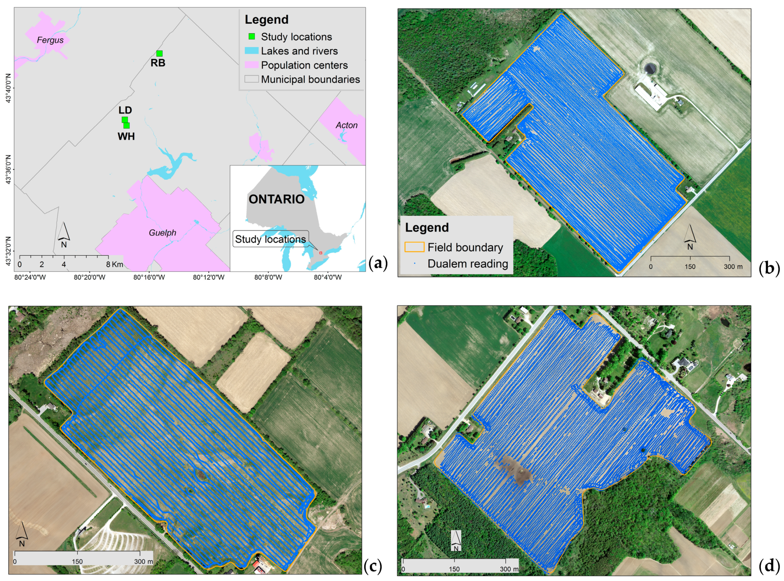
2.1. Experimental Sites and Data Description

Situated at the Woodrill Farms near Guelph, Ontario, Canada, three agricultural fields (namely, WH, LD, and RB), differing in acreage and soil class, were surveyed using both RS and PSS sensors (

Table 1. Characteristics of three agricultural fields in Guelph, Ontario, Canada.

Field ID	Area (ha)	Soil Classes	Target Crops
WH	39.60	Loam	Soybean/Wheat
LD	21.00	Sandy Loam	Soybean
RB	75.00	Fine Sandy Loam	Soybean/Wheat

and Figure 1). The PSS equipment was pulled behind an all-terrain vehicle and measured elevation and EC_a data points for the experimental sites at intra- and inter-row spacings of 5 m and 10 m, respectively. Elevation data points were collected by an RTK Global Navigation Satellite Systems (GNSS) receiver (Trimble Inc., California, USA) (

Table 2. Summary statistics of elevation data from the Real-Time Kinematic (RTK) sensor for three agricultural fields in Guelph, Ontario, Canada.

Field ID	# of Measurements		Elevation (m)
		Min	Median	Max	Range	STD	Mean
WH	28493	372.06	378.07	384.54	12.48	2.33	378.21
LD	7110	332.70	344.86	354.17	21.47	5.76	343.95
RB	20813	358.41	367.67	372.16	13.75	3.63	366.64

). On the basis of the high-density elevation points, a digital elevation model (DEM) was created with a spatial precision of about 2 cm horizontally and 3 cm vertically. Slope, aspect ratio [sin(aspect/2)], and a topographic wetness index (TWI) were derived from a DEM of the study sites. Developed by Beven and Kirkby [45] and serving to investigate hydrological processes controlled by topography, the TWI was determined using the SAGA GIS v.2.4 (University of Hamburg, Germany). The DUALEM-21S system (DUALEM Inc, Milton, ON, Canada) had one transmitter coil and four receivers—two of horizontal coplanar (HCP) geometry and two of perpendicular coplanar (PRP) geometry—at a separation distance of 1 to 2 m. It was used to collect EC_a at four different depths: PRP1 at 0–0.5 m, PRP2 at 0–1.0 m, HCP1 at 0–1.6 m, and HCP2 at 0–3.0 m (

Table 3. Summary of statistics from DUALEM-21S sensor readings from the three agricultural fields. HCP: horizontal coplanar, PRP: perpendicular coplanar.

Field ID	# of Measurements	Sensor Configuration	Apparent Soil Electrical Conductivity (ECa), mS m−1
			Min	Median	Max	Range	STD	Mean
WH	20129	HCP1	4.00	12.28	25.28	21.28	1.69	12.51
LD	6931		2.58	6.90	16.08	13.50	1.55	6.96
RB	18524		1.70	9.00	17.98	16.28	2.81	9.13
WH	20129	PRP1	4.68	7.92	22.24	17.56	1.60	8.15
LD	6931		0.72	4.44	14.12	13.40	1.38	4.55
RB	18524		0.00	3.53	16.80	16.80	2.86	4.40
WH	20129	HCP2	7.42	10.46	24.42	17.00	1.79	10.83
LD	6931		0.50	4.44	14.44	13.94	1.85	4.61
RB	18524		2.50	8.45	14.99	12.49	2.65	8.22
WH	20129	PRP2	5.42	9.10	23.92	18.50	1.75	9.37
LD	6931		1.08	4.68	14.60	13.52	1.50	4.75
RB	18524		0.14	5.10	15.00	14.86	2.96	5.64

). The pre-processing procedures for the collection of RTK elevations and EC_a values were similar and included a raw data display, the identification of missing values, median filtering, and the removal of outliers. Culled data included: (i) start pass and end pass delays, (ii) points with overspeed limits, (iii) values outside the user-defined minimum and maximum values, and (iv) pitch or roll changes outside the acceptable limit. Data outliers were removed on the basis of the criteria above, such that about 15% of data points were removed. Various methods of geospatial data processing were undertaken on multiple data layers, including rectification, interpolation, and point data extraction. These methods enhanced the data quality for further analysis.

A Sentinel-2 image was used to analyze bare soil and vegetation characteristics (

Table 4. Remote sensing data characteristics and their sources.

Satellite Sensor	Spectral Bands	Pixel (m)	Central Wavelength(nm)	Imaging Date	Source
OrthoPhoto	B, G, R, NIR	0.2	-	23 May 2015	OMAFRA/OMNRF 1
Sentinel-2	2(B), 3(G), 4(R), 8(NIR)	10.0	494, 560, 665, 834	21 July 2017	Planet Labs
Sentinel-2	5,6,7 (red edge 1,2 &3)	20.0	704, 740, 781	21 July 2017	Planet Labs

¹ Ontario Ministry of Agriculture, Food and Rural Affairs (OMAFRA) and Ontario Ministry of Natural Resources and Forestry (OMNRF).

). Remote sensing image processing steps were followed, including radiometric correction, stitching, co-registration, and stack bands. One OrthoPhoto and two Sentinel-2 images were used for co-registration and visual interpretation with zonal thematic maps. In addition to the traditional visible (RGB) and near-infrared (NIR) spectral bands, Sentinel-2 imagery presented red edge part of the spectrum as well. Spectral indices were produced from Sentinel-2 data to identify the strong absorption spectrum of chlorophyll. These included the Difference Vegetation Index (DVI), the Normalized Difference Red Edge Index (NDRE), the Normalized Difference Vegetation Index (NDVI), and the Modified Soil Adjusted Vegetation Index (MSAVI2). Among the vegetation indices (VIs), NDVI maps were found to be more suitable and were used for the clustering process [46,47].

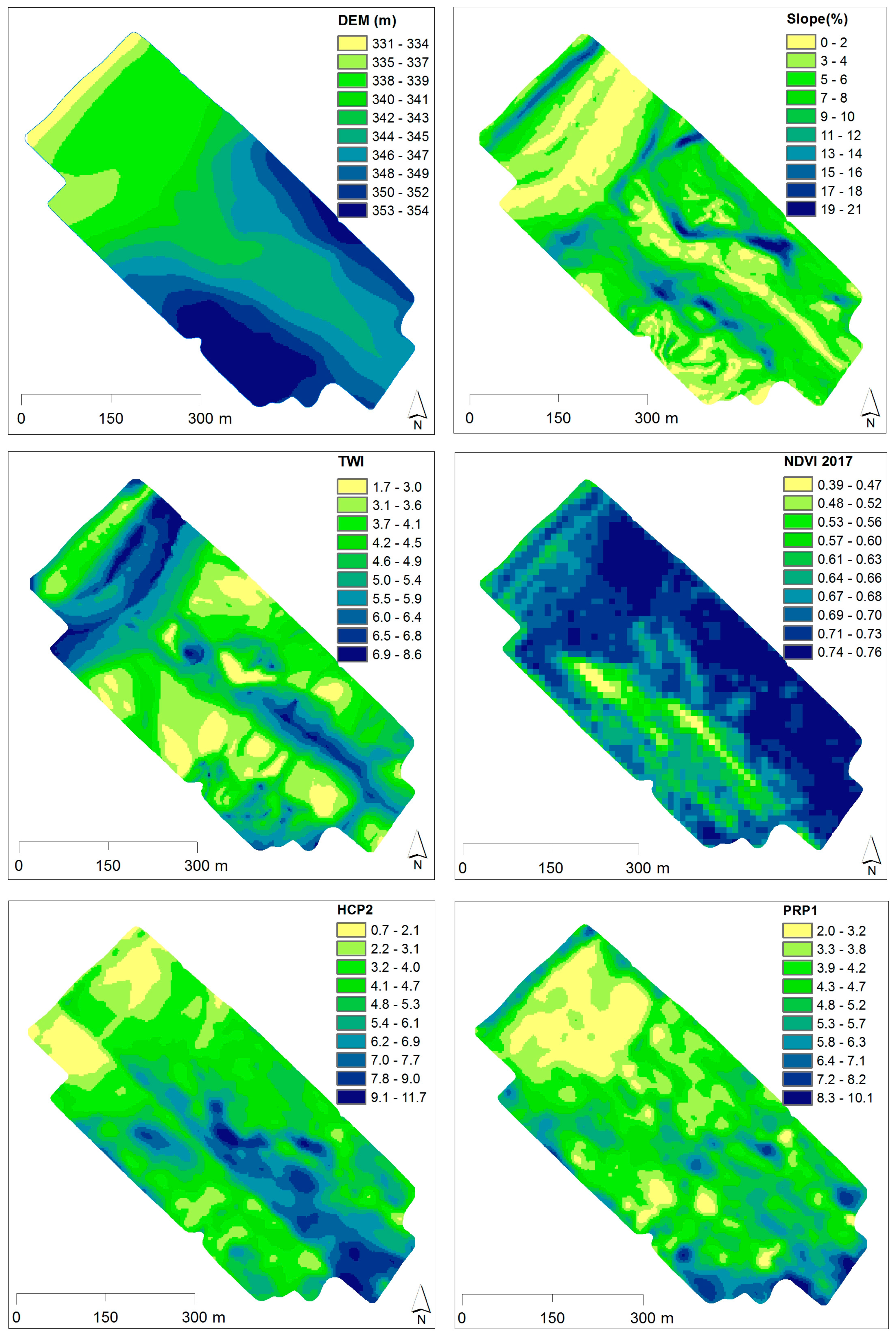
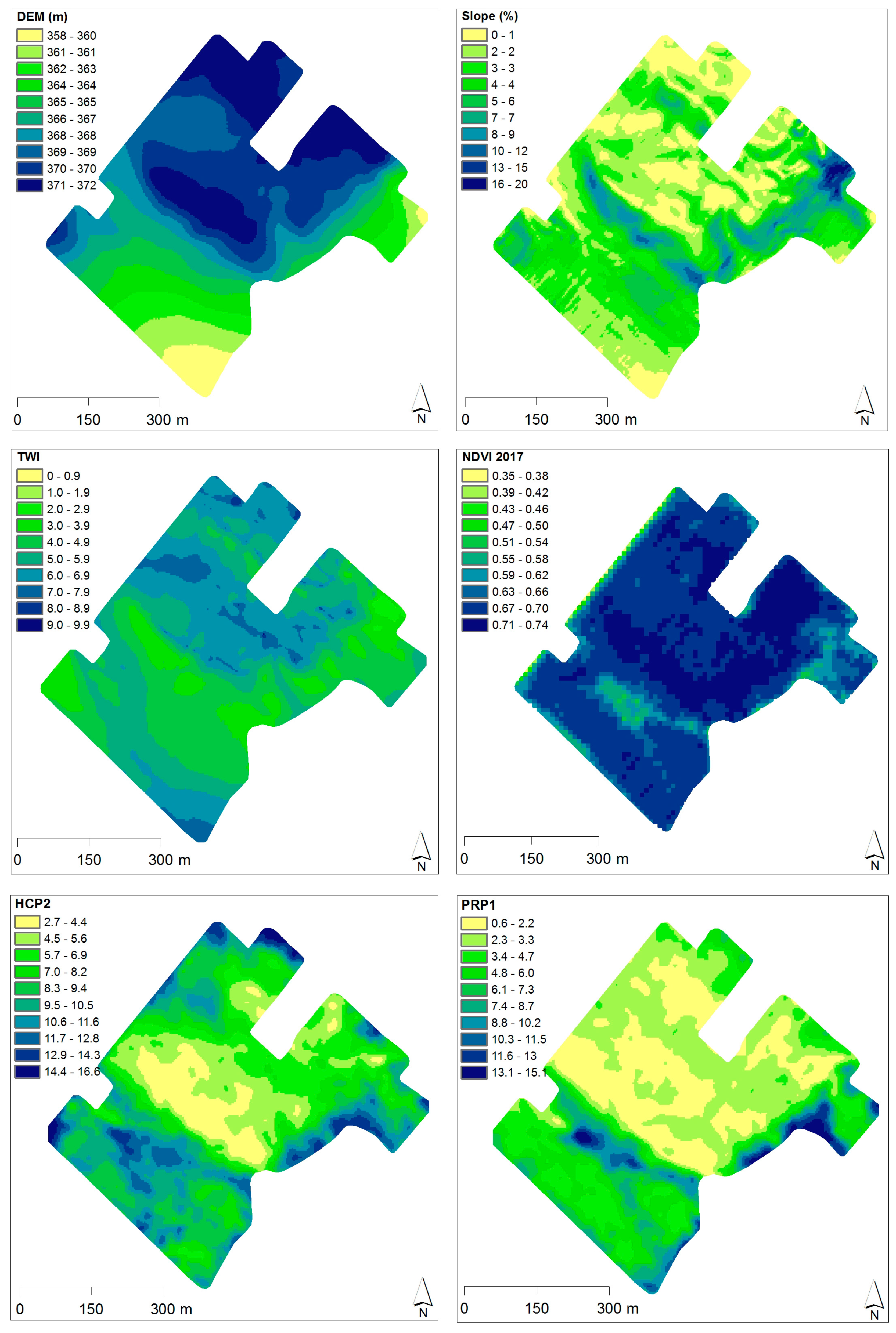
2.2. Interpolated Maps of Selected Sensor Variables

Ordinary Kriging interpolation maps were generated from the PSS measurements in ESRI ArcGIS software (v10.5.1). Kriged maps (with a spatial resolution of 5 m) showing RTK elevation (DEM), derived topographic variables (including slope, aspect, and TWI), and DUALEM sensor variables (HCP1, HCP2, PRP1, and PRP2) were produced. Slope and aspect showed similar clustering patterns as TWI and thus were deemed redundant. In the final clustering process only TWI was used. Indices from NDVI maps (with a spatial resolution of 10 m) were extracted for the clustering tool. Those maps represented significant variations across the expanse of each field (Figure 2, Figure 3 and Figure 4). The interpolated maps were extracted into a data file of multiple layers. Finally, a text data file was generated to store the sensor-derived variables for input into the newly developed clustering tool and commonly used fuzzy clustering techniques.

To delineate zones, the multilayer data files were analyzed by the proposed data clustering tool. The new data clustering algorithm and its processing steps are elaborated in detail in the following section, as well as the new algorithm’s clustering outputs in comparison to outputs from fuzzy clustering techniques.

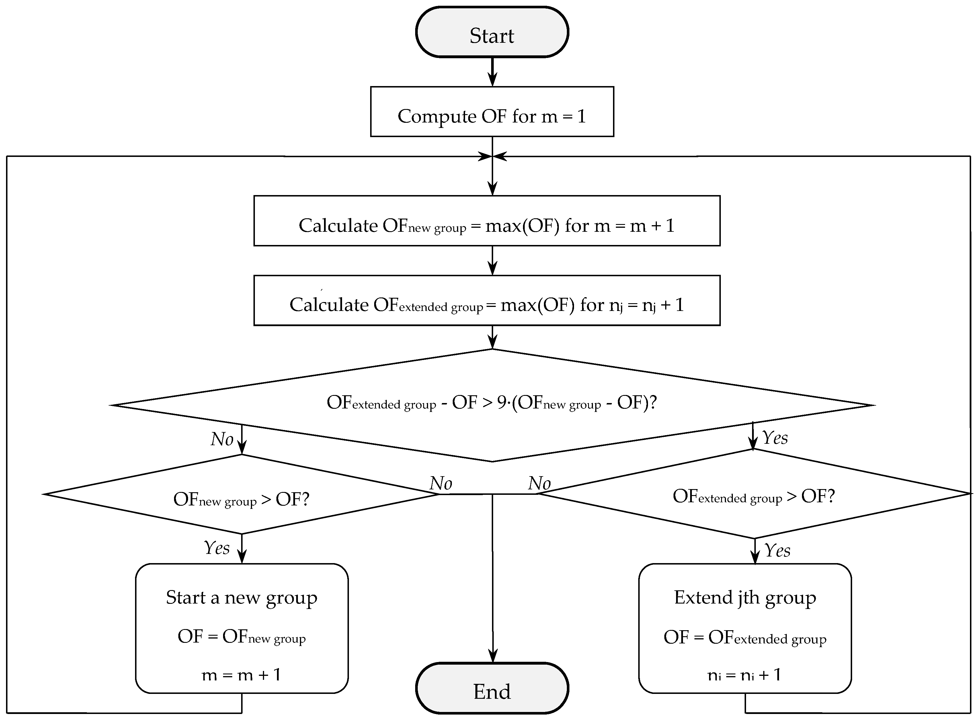
2.3. Data Clustering Algorithms

Fuzzy c-means calculated by the management zone analyst (MZA) [48] were used to generate the normalized classification entropy (NCE) and fuzziness performance index (FPI) of the five zones. The k-means algorithm in the Python data library was used to generate (k = 5, k =15, and k = 25) clusters and find cluster centers using the sum of square distances of all data points and the number of cases in each cluster. Initially, five user-defined clusters were defined in the above clustering methods; however, the optimum number of zones was determined in the final step and compared between the two methods.

The proposed data clustering method, called the Neighborhood Search Analyst (NSA), resulted in the algorithms shown in Figure 5. The processing steps and formula were adopted from the NSA and are written in MATLAB scripts [6]. Preliminary tests of the algorithm in numerous production fields highlighted the algorithm’s robustness when partitioning field areas using several field measurements. To construct an objective function to be optimized through the data grouping process, the mean squared error (MSE) was calculated for each individual data layer k according to:

$$MS{E}_k=\frac{{\displaystyle \sum _{j=1}^m{\displaystyle \sum _{i=1}^{n_j}{\left(X_{ij}-{\overline{X}}_j\right)}^2}}}{N-m}$$

(1)

where X_ij is a sensor value for the i_th grid cells within the j_th group; ${\overline{X}}_j$ is the mean of j_th group; N is the total number of grid cells; m is the number of groups; and n_j is the number of grid cells within the j_th group.

It should be noted that the difference between the total number of grid cells and the number of groups can be determined by:

$$N-m={\displaystyle \sum _{j=1}^m\left(n_j-1\right)}$$

(2)

Since the algorithm initially assumes that all grid cells belong to the same group, labeled “1” and designated as "the rest of the field", then MSE_k(m = 1) represents the variance of the k_th data layer across the entire field. Given that the area of the field is substantially greater than the area of a grid cell, MSE_k(m = 1) can be termed Farthest Distance Variance (FDV_k). In such a situation, the portion of data variance accounted for by distributing N grid cells among m groups can be calculated as:

$$R_k^2=1-\frac{MS{E}_k}{FD{V}_k}$$

(3)

where MSE_k(m = 1) can be called Farthest Distance Variance (FDV_k).

The maximum value of R²_k can be obtained when MSE_k is as small as possible. It approaches 1when the number of groups increases. Since the result can be considered less favorable if at least one data layer k is not adequately accounted for, it is reasonable to employ the integration operator OR instead of the more common AND. This avoids the need to assign a weight factor to each individual data layer when adding corresponding MSE_k estimates. In mathematical terms, this would mean that the product of all R²_k should be maximized. Therefore, the objective function (OF) was defined as:

$$OF={\displaystyle \prod _{k=1}^K{R}_{{}^k}^2}$$

(4)

where K is the number of PSS data layers.

In this study, the smallest number of data elements that could be grouped within the grid cell square window was nine (3 × 3). Therefore, the maximum accountable variance is the variance of PSS measurements between immediate neighbors. The Shortest Distance Variances (SDV_k) can be found using:

$$SD{V}_k=\frac{1}{w}{\displaystyle \sum _{j=1}^w{\displaystyle \sum _{i=1}^9\frac{{\left(X_{ij}-{\overline{X}}_j\right)}^2}{8}}}$$

(5)

where w is the total number of 3 × 3 square windows of grid cells.

Since SDV_k represents the smallest MSE_k value, the maximum value of R²_k is calculated as:

$${R_k^2}_{\max }=1-\frac{SD{V}_k}{FD{V}_k}$$

(6)

This R²_{k max} parameter can range between 0 and 1. It is equal to 0 when data layer k is either uniform or highly variable, so that SDV_k = FDV_k. In such a case, the data layer should not be able to affect changes in the OF. Alternatively, when R²_{k max} is close to 1, the data layer has a strong spatial structure (SDV_k << FDV_k), and OF must be sensitive to the change of MSE_k corresponding to that particular data layer. In mathematical terms, this goal can be achieved by multiplying all R²_k values raised to the R²_{k max} power of:

$$OF={{\displaystyle \prod _{k=1}^K{R}_{{}^k}^2}}^{R_{k\max }^2}={{\displaystyle \prod _{k=1}^K\left(1-\frac{MS{E}_k}{FD{V}_k}\right)}}^{\left(1-\frac{SD{V}_k}{FD{V}_k}\right)}$$

(7)

The resultant OF indicates the overall quality of grid cell groupings. It varies from 0 to 1 and approaches high values when every spatially structured layer of PSS measurement is separated among spatially continuous groups of grid cells with minimum internal group variance. Such groups represent different combinations of average PSS measurements obtained with different sensors that diverge from average field conditions. To facilitate the formation of grid cell groups that would maximize the OF, the NSA algorithm was implemented in this study using Python v3.6 (created by Guido van Rossum and managed by Python Software Foundation, Delaware, USA).

3. Results and Discussion

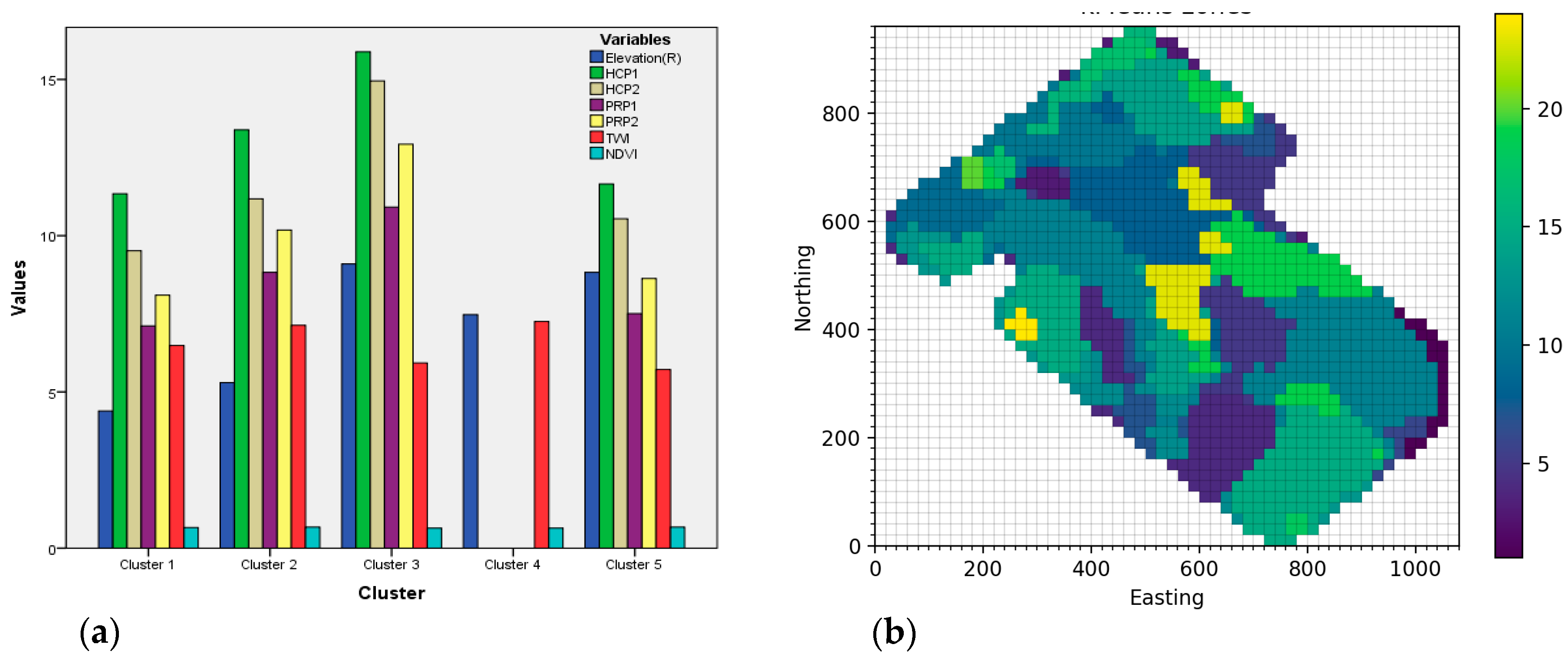
3.1. c-Means Clustering

On the basis of the seven input variables (i.e., elevation, TWI, NDVI, HCP1, HCP2, PRP1, and PRP2) of the WH field, Euclidean distance-based NCE and FPI indices in FCM clustering were assessed for their performance in creating an optimum number of zones. Comparing the NCE index to the FPI index showed that the maximum value was reached only in zones 4 and 5 (Figure 6). This clustering method is flaws when it comes to obtaining an optimum number of zones [8,49,50]. The FCM clusters produced pixels with isolated boundaries in various parts of the field [51,52]. Many studies have reported this representation problem regarding the clustering of data due to the fuzzy boundary [16,32,53,54]. In the present method, user-defined numbers of clusters were produced without considering the geospatial locations of the dataset (spatial continuity) or their distances.

3.2. k-Means Clustering

In the k-means clustering (k=5), the data values were taken directly from the input table of the WH field for generating cluster centers (Figure 7a). Data were standardized and normalized for the specific variable values. Among the five user-defined clusters, clusters 1, 2, 3, and 5 used the most data points. Since there was a random component, after several runs of each clustering process, the coefficient of determination (R²) varied according to how the k-means algorithm was initialized. The cluster map consisted of groups of pixels with isolated boundaries in various parts of the WH field (Figure 7b). Figure 7b shows that the k-means cluster map of the WH field generated 36 scattered zones of user-define clusters (k=25).

3.3. NSA Clustering

In the NSA zone delineation process, unlike other clustering algorithms, providing the number of field partitioning clusters is not obligatory. Without defining the number of clusters, NSA produced an optimum number of groups for the grid cell (grid size of 20 m), separately, for seven different input variables. More importantly, this clustering tool efficiently delimited maps by providing the optimum number of zones for field management (Figure 8a, Figure 9a and Figure 10a). On this basis, the WH, LD, and RB fields have 28, 20, and 27 georeferenced zones, respectively. For NSA clustering, user-defined (k = 5, k = 15, and k = 25) zones were delineated and are illustrated later in this paper.

In NSA, zone delineation was performed by the individual R² values of each variable (Figure 8b, Figure 9b and Figure 10b) and overall OF (Figure 8c, Figure 9c and Figure 10c). These graphs show the part of the variance of each data layer which was accounted for by subdividing the field into smaller areas. In each graph, a greater number of R² value indicated that variability within individual zones was smaller than the difference between zones. Figure 8b, Figure 9b and Figure 10b show that the R² values increased when new groups were formed or added to the existing groups. The NSA that produced R²_max value was about 0.9, and the graph had a steeper initial slope. This indicated that the data layer had a strong spatial structure and was dominant when the field was split. Moreover, the x value (No. of cells), where most graphs leveled off, showed that the smallest level of field partitioning revealed most of the soil heterogeneity. Results in LD and RB fields indicated that R² for each data layer reached a maximum height (0.60) with around 500 classified grid cells, whereas R² reached 0.70 near the 1000-grid cell level for the WH field (Figure 11). Roughly 60% (in LD and RB) and 70% (WH) of the field variance in both cases was accounted for by making the clusters.

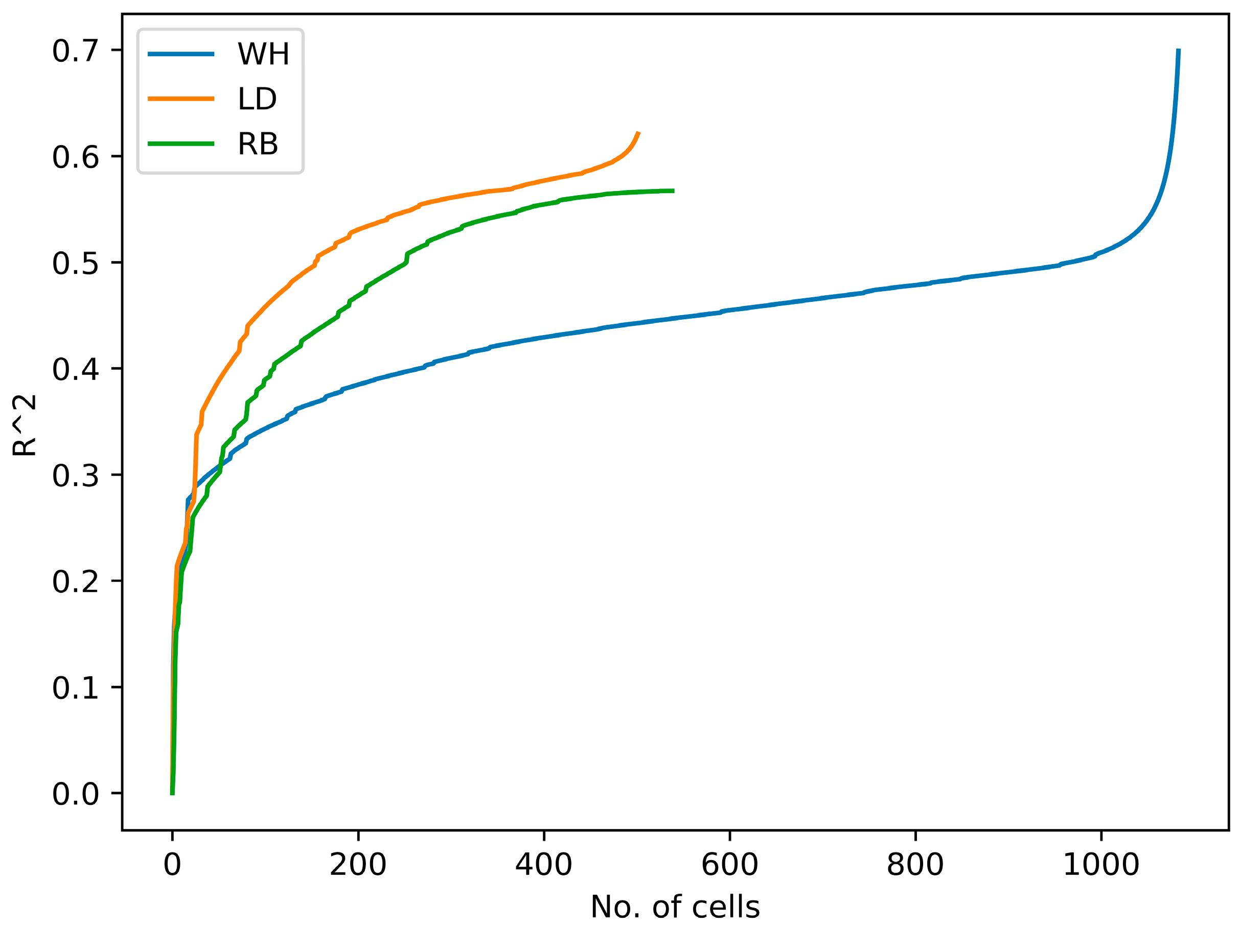
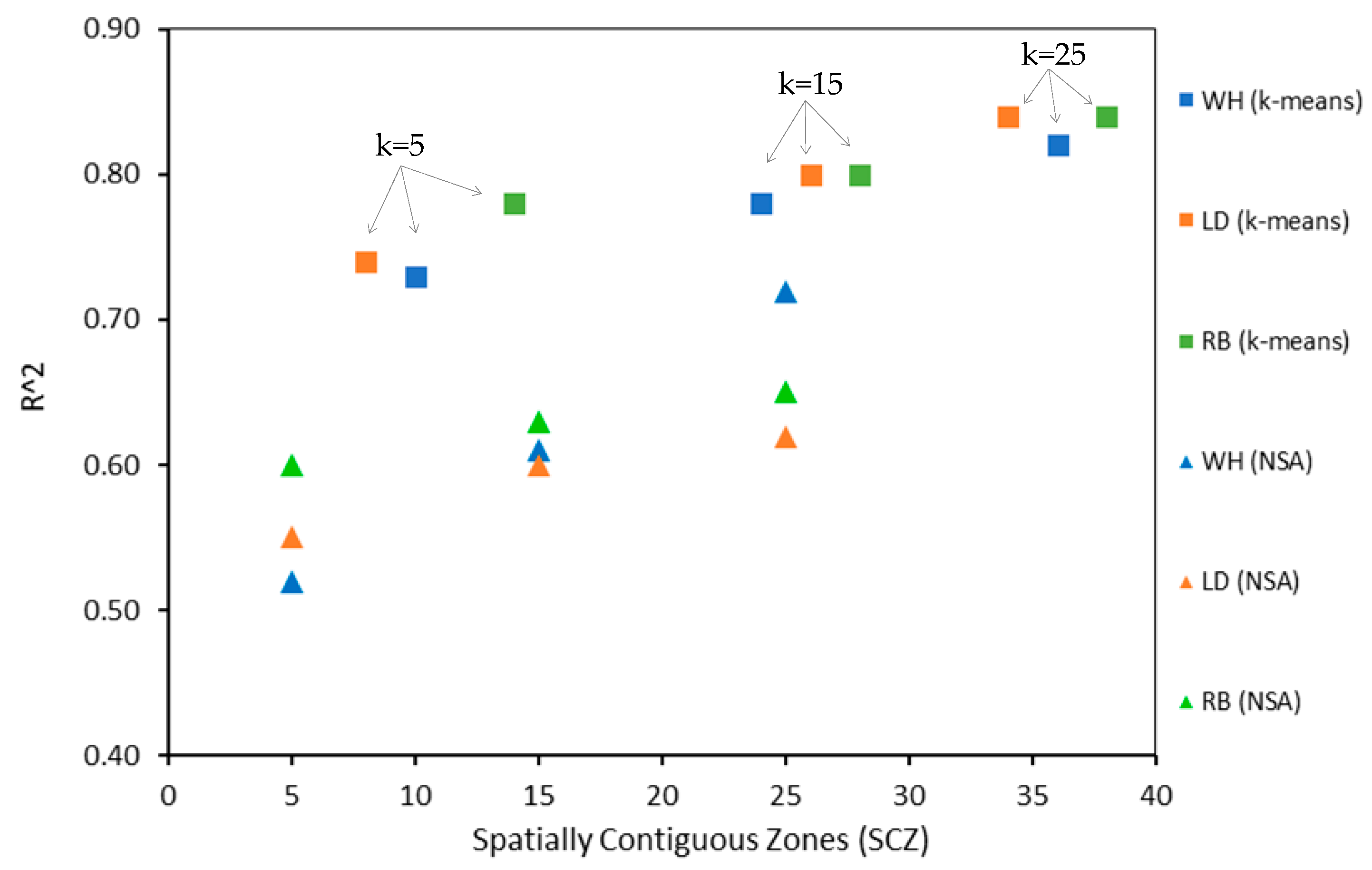
3.4. Comparison of k-Means and NSA Clustering

At this stage, three user-defined clusters (k = 5, k = 15, and k = 25) were generated to allow a comparison of the two clustering algorithms, i.e., k-means and NSA. User-defined centers for all clusters were needed for k-means; however, these were not a requirement for the NSA algorithm. The R² values of the NSA algorithm were compared among the three different fields (Figure 11). The overall OF showed that all of the clusters reached maximum R² values close to 0.6 and up to 0.7. In the three defined k-means clusters (k = 5, k = 15, and k = 25), the R² of the RB field was higher: 0.78, 0.80, and 0.84 respectively (Figure 12). Also, R² (k = 5) was relatively high in k-means clustering process because of the fragmentation of clusters throughout the field, while NSA clusters were always contiguous (i.e., not broken into parts). The R² of the k-means cluster compared to that of the NSA was higher in most of the fields and was approximately 0.80. The R² values were comparable when the isolated/boundary pixels in each k-means cluster were disjointed from the main cluster and created spatially contiguous zones. The k-means cluster map consisted of groups or pixels with isolated boundaries in various parts of the WH field (Figure 7b), whereas the NSA algorithm counted these as different groups and reduced the zone fragmentation (Figure 8a). In the case of the user-defined cluster (k = 25), the k-means cluster maps of WH, LD, and RB fields generated 36, 34, and 38 scattered zones respectively, whereas the NSA maps created approximately 25 spatially contiguous clusters for each of the three fields (Figure 12).

4. Conclusions

The high-density and multivariate data clustering approach provided an optimal number of zones for three agricultural fields in Ontario, Canada. The preprocessing and variable selection steps common to all clustering techniques are imperative for providing a well-defined zonal boundary for developing management zones. Compared to other data clustering algorithms, NSA has a unique capability for zone separation, which allows one to produce an optimum number of zones and spatially contiguous clusters during multivariate classification. Moreover, an improved version of this software was tested and proved to be capable of handling a significant number of variables and data layers for delineating the optimum number of zones in a more robust way.

The software was found to be reliable when integrating high-density field topography, RS, and PSS data files. It had a fast processing time and could be run on any platform with open source python modules. The robust zone delineation process and georeferenced thematic maps are useful for variable rate crop management technologies and for other management purposes. Multi-sensor data fusion, advanced data filtering procedures, and the web application of the NSA could be implemented to facilitate appropriate site-specific agronomic and environmental decisions in many regions.

The zonal maps will be useful for further agronomic model calibration using targeted soil sampling. Field data, for example, crop yield and lab-measured soil properties, could be used to validate the georeferenced clusters and management zones created. Furthermore, this research enhances and provides information for better variable-rate fertilizer recommendations and can optimize pesticide and herbicide applications, thereby providing greater environmental benefits.

References

1. Zhang, N.; Wang, M.; Wang, N. Precision Agriculture—A Worldwide Overview. Comput. Electron. Agric. 2002, 36, 113–132. [Google Scholar] [CrossRef]
2. Shatar, T.M.; McBratney, A. Subdividing a Field into Contiguous Management Zones Using a K-Zones Algorithm. In 3rd European Conference on Precision Agriculture; Grenier, G., Blackmore, S., Eds.; Agro-Montpellier ENSAM: Montpellier, France, 2001; pp. 115–120. [Google Scholar]
3. Fridgen, J.J.; Kitchen, N.R.; Sudduth, K.A.; Drummond, S.T.; Wiebold, W.J.; Fraisse, C.W. Management Zone Analyst (MZA): Software for Subfield Management Zone Delineation. Agron. J. 2004, 96, 100–108. [Google Scholar] [CrossRef]
4. Khosla, R.; Westfall, D.G.; Reich, R.M.; Mahal, J.S.; Gangloff, W.J. Spatial Variation and Site-Specific Management Zones. In Geostatistical Applications for Precision Agriculture; Oliver, M.A., Ed.; Springer Science: Berlin, Germany, 2010; pp. 195–219. [Google Scholar]
5. De Benedetto, D.; Castrignano, A.; Diacono, M.; Rinaldi, M.; Ruggieri, S.; Tamborrino, R. Field Partition by Proximal and Remote Sensing Data Fusion. Biosyst. Eng. 2013, 114, 372–383. [Google Scholar] [CrossRef]
6. Dhawale, N.M.; Adamchuk, V.I.; Prasher, S.O.; Dutilleul, P.R.L.; Ferguson, R.B. Spatially Constrained Geospatial Data Clustering for Multilayer Sensor-Based Measurements. In Geospatial Theory, Processing, Modeling and Applications; ISPRS Technical Commission II Symposium: Toronto, ON, Canada, 2014; Volume 40, pp. 187–190. [Google Scholar]
7. Castrignanò, A.; Buttafuoco, G.; Quarto, R.; Vitti, C.; Langella, G.; Terribile, F.; Venezia, A. A Combined Approach of Sensor Data Fusion and Multivariate Geostatistics for Delineation of Homogeneous Zones in an Agricultural Field. Sensors (MDPI) 2017, 17, 2794. [Google Scholar] [CrossRef] [PubMed]
8. Albornoz, E.M.; Kemerer, A.C.; Galarza, R.; Mastaglia, N.; Melchiori, R.; Martínez, C.E. Development and Evaluation of an Automatic Software for Management Zone Delineation. Precis. Agric. 2018, 19, 463–476. [Google Scholar]
9. Deng, X.; Wang, Y.; Peng, H. Clustering of High-Resolution Remote Sensing Imagery. In Third International Asia-Pacific Environmental Remote Sensing Remote Sensing of the Atmosphere, Ocean, Environment, and Space; Ungar, S., Mao, S., Yasuoka, Y., Eds.; SPIE: Hangzhou, China, 2003. [Google Scholar]
10. Adamchuk, V.I.; Hummel, J.W.; Morgan, M.T.; Upadhyaya, S.K. On-the-Go Soil Sensors for Precision Agriculture. Comput. Electron. Agric. 2004, 44, 71–91. [Google Scholar] [CrossRef]
11. Berkhin, P. A Survey of Clustering Data Mining Techniques. In Grouping Multidimensional Data; Springer: Berlin/Heidelberg, Germany, 2006; pp. 25–71. [Google Scholar] [Green Version]
12. Cohen, S.; Cohen, Y.; Alchanatis, V.; Levi, O. Combining Spectral and Spatial Information from Aerial Hyperspectral Images for Delineating Homogenous Management Zones. Biosyst. Eng. 2013, 114, 435–443. [Google Scholar] [CrossRef]
13. De Benedetto, D.; Castrignanò, A.; Rinaldi, M.; Ruggieri, S.; Santoro, F.; Figorito, B.; Gualano, S.; Diacono, M.; Tamborrino, R. An Approach for Delineating Homogeneous Zones by Using Multi-Sensor Data. Geoderma 2013, 199, 117–127. [Google Scholar] [CrossRef]
14. McBratney, A.B.; Mendonça Santos, M.L.; Minasny, B. On Digital Soil Mapping. Geoderma 2003, 117, 3–52. [Google Scholar] [CrossRef]
15. Vrindts, E.; Mouazen, A.M.; Reyniers, M.; Maertens, K.; Maleki, M.R.; Ramon, H.; De Baerdemaeker, J. Management Zones Based on Correlation between Soil Compaction, Yield and Crop Data. Biosyst. Eng. 2005, 92, 419–428. [Google Scholar] [CrossRef]
16. Yan, L.; Zhou, S.; Feng, L. Delineation of Site-Specific Management Zones Based on Temporal and Spatial Variability of Soil Electrical Conductivity. Pedosphere 2007, 17, 156–164. [Google Scholar]
17. Cressie, N.; Kang, E.L. High-Resolution Digital Soil Mapping: Kriging for Very Large Datasets. In Proximal Soil Sensing; Viscarra Rossel, R.A., McBratney, A.B., Minasny, B., Eds.; Springer: Dordrecht, The Netherlands, 2010; pp. 49–63. [Google Scholar]
18. Jiang, Q.; Fu, Q.; Wang, Z. Study on Delineation of Irrigation Management Zones Based on Management Zone Analyst Software. In International Conference on Computer and Computing Technologies in Agriculture; Springer: Berlin/Heidelberg, Germany, 2010; pp. 419–427. [Google Scholar]
19. Adamchuk, V.I.; Viscarra Rossel, R.A. Precision Agriculture: Proximal Soil Sensing. In Encyclopedia of Agrophysics; Gliński, J., Horabik, J., Lipiec, J., Eds.; Springer: Dordrecht, The Netherlands, 2011; pp. 650–656. [Google Scholar]
20. Dhawale, N.; Adamchuk, V.; Huang, H.; Ji, W.; Lauzon, S.; Biswas, A.; Dutilleul, P. Integrated Analysis of Multilayer Proximal Soil Sensing Data. In Proceedings of the International Conference on Precision Agriculture, St. Louis, MO, USA, 31 July–4 August 2016. [Google Scholar]
21. Samet, H. An Overview of Hierarchical Spatial Data Structures. In Proceedings of the Fifth Israeli Symposium on Artificial Intelligence, Vision, and Pattern Recognition, Tel-Aviv, Ganei-Hata’arucha, Israel, 27–28 December 1988; pp. 331–351. [Google Scholar]
22. Arabie, P.; Hubert, L.J. An Overview of Combinatorial Data Analysis. In Clustering and Classification; Arabie, P., Soete, G.D., Hubert, L.J., Eds.; World Scientific Pub. Co.: Singapore, 1996; pp. 5–63. [Google Scholar]
23. Fisher, D. Iterative Optimization and Simplification of Hierarchical Clustering. J. Artif. Intell. Res. 1996, 4, 147–178. [Google Scholar] [CrossRef]
24. Burrough, P.A.; Van Gaans, P.F.M.; Hootsmans, R. Continuous Classification in Soil Survey: Spatial Correlation, Confusion and Boundaries. Geoderma 1997, 77, 115–135. [Google Scholar] [CrossRef]
25. Ruß, G.; Brenning, A. Data Mining in Precision Agriculture: Management of Spatial Information. In Computational Intelligence for Knowledge-Based Systems Design; Hüllermeier, E., Kruse, R., Hoffmann, F., Eds.; Springer: Berlin/Heidelberg, Germany, 2010; pp. 350–359. [Google Scholar]
26. Johnson, S.C. Hierarchical Clustering Schemes. Psychometrika 1967, 32, 241–254. [Google Scholar] [CrossRef] [PubMed]
27. Sadahiro, Y. Cluster Perception in the Distribution of Point Objects. Cartogr. Int. J. Geogr. Inf. Geovisualization 1997, 34, 49–62. [Google Scholar] [CrossRef]
28. Fraisse, C.W.; Sudduth, K.A.; Kitchen, N.R. Delineation of Site-Specific Management Zones by Unsupervised Classification. Trans. ASAE 2001, 44, 155–166. [Google Scholar] [CrossRef]
29. Motwani, M. A Study on Initial Centroids Selection for Partitional Clustering Algorithms. Adv. Intell. Syst. Comput. 2019, 731, 211–220. [Google Scholar]
30. De Gruijter, J.J.; Walvoort, D.J.J.; Van Gaans, P.F.M. Continuous Soil Maps—A Fuzzy Set Approach to Bridge the Gap between Aggregation Levels of Process and Distribution Models. Geoderma 1997, 77, 169–195. [Google Scholar] [CrossRef]
31. Gui-Fen, C.; Li-Ying, C.; Guo-Wei, W.; Bao-Cheng, W.; Da-You, L.; Sheng-Sheng, W. Application of a Spatial Fuzzy Clustering Algorithm in Precision Fertilisation. N. Z. J. Agric. Res. 2007, 50, 1249–1254. [Google Scholar] [CrossRef]
32. Panda, S.; Sahu, S.; Jena, P.; Chattopadhyay, S. Comparing Fuzzy-C Means and K-Means Clustering Techniques: A Comprehensive Study. Adv. Intell. Soft Comput. 2012, 166, 451–460. [Google Scholar]
33. Orhan, U.; Hekim, M.; Ozer, M. EEG Signals Classification Using the K-Means Clustering and a Multilayer Perceptron Neural Network Model. Expert Syst. Appl. 2011, 38, 13475–13481. [Google Scholar] [CrossRef]
34. Saifuzzaman, M.; Adamchuk, V.; Huang, H.-H.; Ji, W.; Rabe, N.; Biswas, A. Data Clustering Tools for Understanding Spatial Heterogeneity in Crop Production by Integrating Proximal Soil Sensing and Remote Sensing Data. In Proceedings of the 14th International Conference on Precision Agriculture, Montreal, QC, Canada, 24–27 June 2018; International Society of Precision Agriculture: Monticello, IL, USA; p. 14. Available online: http://www.ispag.org (accessed on 20 June 2018).
35. Ester, M.; Kriegel, H.-P.; Sander, J.; Xu, X. Density-Based Clustering Algorithms for Discovering Clusters. In Proceedings of the 2nd International Conference on Knowledge Discovery and Data Mining (KDD-96), Portland, OR, USA, 2–4 August 1996; pp. 226–231. [Google Scholar]
36. Liu, Y.; Xiong, N.; Zhao, Y.; Vasilakos, A.V.; Gao, J.; Jia, Y. Multi-Layer Clustering Routing Algorithm for Wireless Vehicular Sensor Networks. IET Commun. 2010, 4, 810. [Google Scholar] [CrossRef]
37. Viscarra Rossel, R.A.; Adamchuk, V.I.; Sudduth, K.A.; McKenzie, N.J.; Lobsey, C. Proximal Soil Sensing: An Effective Approach for Soil Measurements in Space and Time. Adv. Agron. 2011, 113, 237–283. [Google Scholar]
38. Córdoba, M.A.; Bruno, C.I.; Costa, J.L.; Peralta, N.R.; Balzarini, M.G. Protocol for Multivariate Homogeneous Zone Delineation in Precision Agriculture. Biosyst. Eng. 2016, 143, 95–107. [Google Scholar] [CrossRef]
39. González-Fernández, A.B.; Rodríguez-Pérez, J.R.; Ablanedo, E.S.; Ordoñez, C. Vineyard Zone Delineation by Cluster Classification Based on Annual Grape and Vine Characteristics. Precis. Agric. 2017, 18, 525–573. [Google Scholar] [CrossRef]
40. Lazarevic, A.; Xu, X.; Fiez, T.; Obradovic, Z. Clustering-Regression-Ordering Steps for Knowledge Discovery in Spatial Databases. In Proceedings of the International Joint Conference on Neural Networks, Washington, DC, USA, 10–16 July 1999; pp. 2530–2534. [Google Scholar]
41. Walters, R.W.; Jenq, R.R.; Hall, S.B. Evaluating Farmer Defined Management Zone Maps for Variable Rate Fertilizer Application. Precis. Agric. 2000, 2, 201–215. [Google Scholar]
42. Khosla, R.; Fleming, K.; Delgado, J.A.; Shaver, T.M.; Westfall, D.G. Use of Site-Specific Management Zones to Improve Nitrogen Management for Precision Agriculture. J. Soil Water Conserv. 2002, 57, 513–518. [Google Scholar]
43. Mondal, P.; Jain, M.; Defries, R.S.; Galford, G.L.; Small, C. Sensitivity of Crop Cover to Climate Variability: Insights from Two Indian Agro-Ecoregions. J. Environ. Manag. 2014, 148, 21–30. [Google Scholar] [CrossRef]
44. Huang, Y.; Lan, Y.; Thomson, S.J.; Fang, A.; Hoffmann, W.C.; Lacey, R.E. Development of Soft Computing and Applications in Agricultural and Biological Engineering. Comput. Electron. Agric. 2010, 71, 107–127. [Google Scholar] [CrossRef]
45. Beven, K.J.; Kirkby, M.J. A physically based, variable contributing area model of basin hydrology/Un modèle à base physique de zone d’appel variable de l’hydrologie du bassin versant. Hydrol. Sci. Bull. 1979, 24, 43–69. [Google Scholar] [CrossRef]
46. Roberts, D.F.; Adamchuk, V.I.; Shanahan, J.F.; Ferguson, R.B.; Schepers, J.S. Estimation of Surface Soil Organic Matter Using a Ground-Based Active Sensor and Aerial Imagery. Precis. Agric. 2011, 12, 82–102. [Google Scholar] [CrossRef]
47. Viña, A.; Gitelson, A.A.; Nguy-robertson, A.L.; Peng, Y. Remote Sensing of Environment Comparison of Different Vegetation Indices for the Remote Assessment of Green Leaf Area Index of Crops. Remote Sens. Environ. 2011, 115, 3468–3478. [Google Scholar] [CrossRef]
48. U.S. Department of Agriculture (USDA). Management Zone Analyst Version 1.0 Software; U.S. Department of Agriculture: Washington, DC, USA, 2000.
49. GNip, P.G.; Harvát, K.C. Management of Zones in Precision Farming. Agric. Econ. 2003, 49, 416–418. [Google Scholar] [CrossRef]
50. Hartigan, J.A.; Wong, M.A. A K-Means Clustering Algorithm. Appl. Stat. 2012, 28, 100–108. [Google Scholar] [CrossRef]
51. Nazeer, K.A.A.; Sebastian, M.P. Improving the Accuracy and Efficiency of the k-Means Clustering Algorithm. Proc. World Cong. Eng. 2009, I, 1–5. [Google Scholar]
52. Vendrusculo, L.G.; Kaleita, A.F. Modeling Zone Management in Precision Agriculture through Fuzzy C-Means Technique at Spatial Database. In Proceedings of the Agricultural and Biosystems Engineering Conference, Louisville, KY, USA, 8–10 August 2011; Volume 4, pp. 2701–2715. [Google Scholar]
53. Bragato, G. Fuzzy Continuous Classification and Spatial Interpolation in Conventional Soil Survey for Soil Mapping of the Lower Piave Plain. Geoderma 2004, 118, 1–16. [Google Scholar] [CrossRef]
54. Yan, L.; Zhou, S.; Feng, L.; Hong-Yi, L. Delineation of Site-Specific Management Zones Using Fuzzy Clustering Analysis in a Coastal Saline Land. Comput. Electron. Agric. 2007, 56, 174–186. [Google Scholar]
Figure 1. (a) Location and aerial views of three fields at the Woodrill Farms in Guelph Ontario, Canada: WH field boundary with soil apparent electrical conductivity (ECa) data points (b), LD field boundary with soil ECa data points (c), and RB field boundary with soil ECa data points (d).
Remotesensing 11 01036 g001
Figure 2. Interpolated maps (Kriged) of digital elevation model (DEM), topographic wetness index (TWI), HCP2, PRP1, and Normalized Difference Vegetation Index (NDVI) maps for the WH field.
Remotesensing 11 01036 g002
Figure 3. Interpolated maps (Kriged) of DEM, TWI, HCP2, PRP1, and NDVI maps for the LD field.
Remotesensing 11 01036 g003
Figure 4. Interpolated maps (Kriged) of DEM, TWI, HCP2, PRP1, and NDVI maps for the RB field.
Remotesensing 11 01036 g004
Figure 5. The flowchart of the Neighborhood Search Analyst (NSA) algorithm process.
Remotesensing 11 01036 g005
Figure 6. Normalized classification entropy (NCE) (a) and fuzziness performance index (FPI) (b) of the WH field based on seven input variables.
Remotesensing 11 01036 g006
Figure 7. (a) k-means cluster (k = 5) centers with variable values of the WH field and (b) k-means cluster (k = 25) map of the WH field showing zones with various isolated pixels.
Remotesensing 11 01036 g007
Figure 8. (a) Zonal map including 28 well-defined clusters; (b) Coefficient of determination (R2) for each data layer; and (c) Overall objective function (OF) vs number of grid cells (WH).
Remotesensing 11 01036 g008
Figure 9. (a) Zonal map including 20 well-defined clusters; (b) Coefficient of determination (R2) for each data layer; and (c) Overall OF vs number of grid cells (LD).
Remotesensing 11 01036 g009
Figure 10. (a) Zonal map including 27 well-defined clusters; (b) Coefficient of determination (R2) for each data layer; and (c) Overall OF vs number of grid cells (RB).
Remotesensing 11 01036 g010
Figure 11. Comparison of R2 value for NSA clustering for WH, LD, and RB fields.
Remotesensing 11 01036 g011
Figure 12. Comparison of R2 value between k-means and NSA clustering. The abscissa (SCZ) shows the number of spatially contiguous zones created when k = 5, k = 15, and k = 25.
Remotesensing 11 01036 g012