Filtering Airborne LiDAR Data Through Complementary Cloth Simulation and Progressive TIN Densification Filters

 , , and
Abstract
1. Introduction
2. Test Data
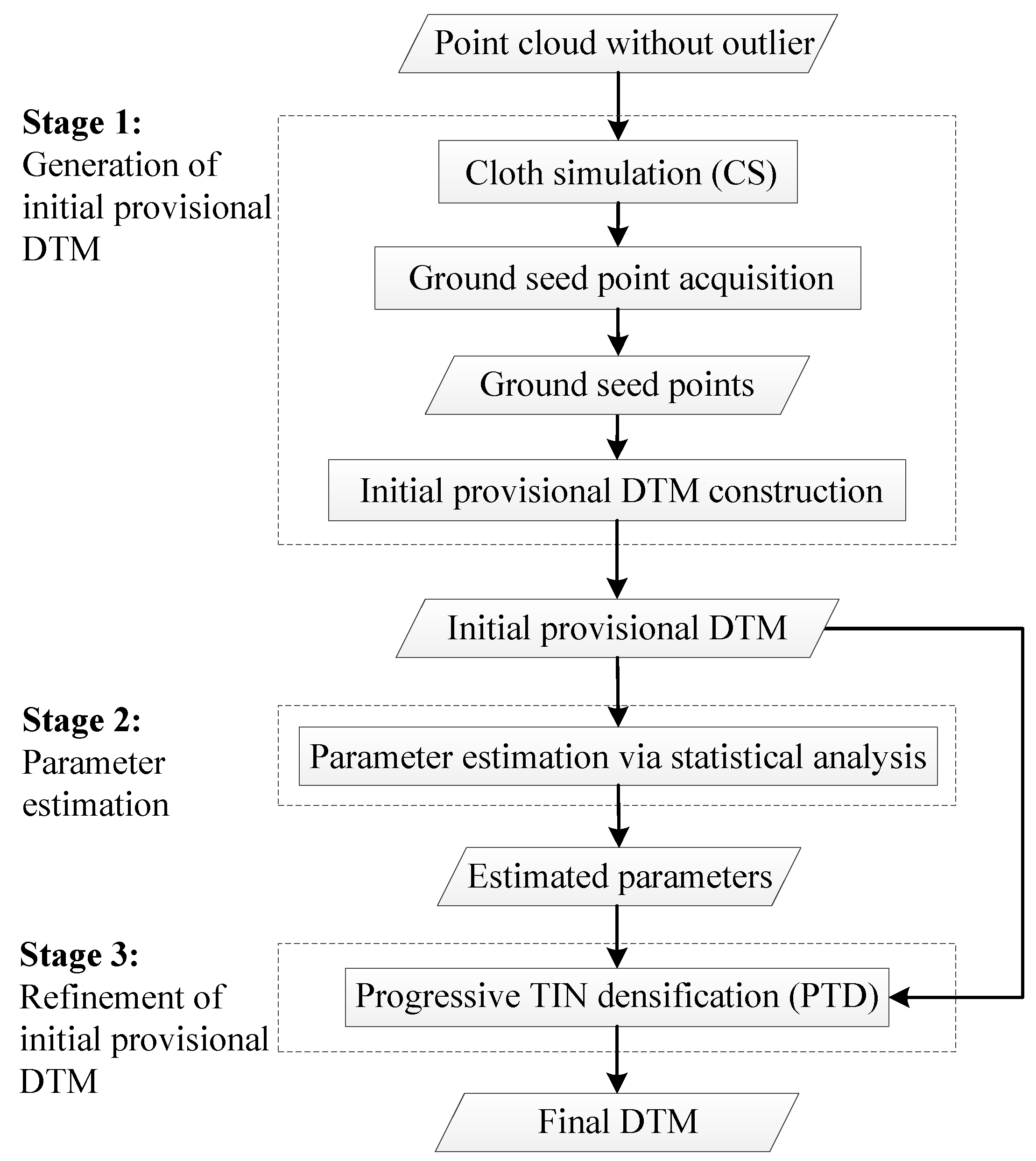
3. Methods
3.1. Generation of Initial Provisional DTM Based on Cloth Simulation
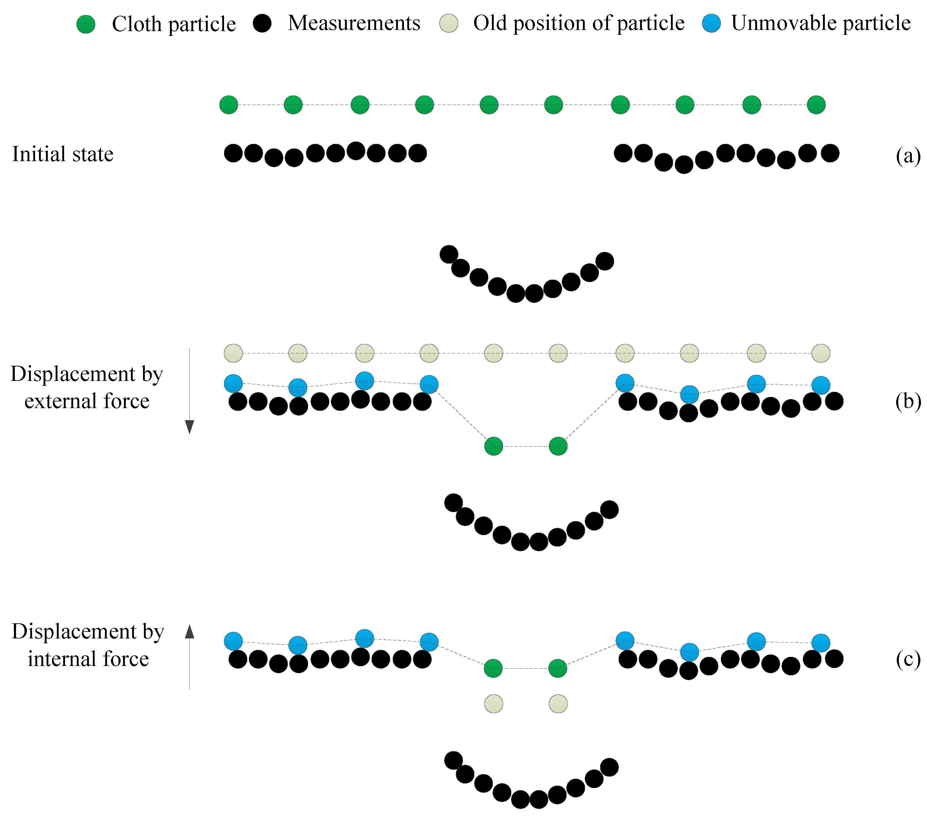
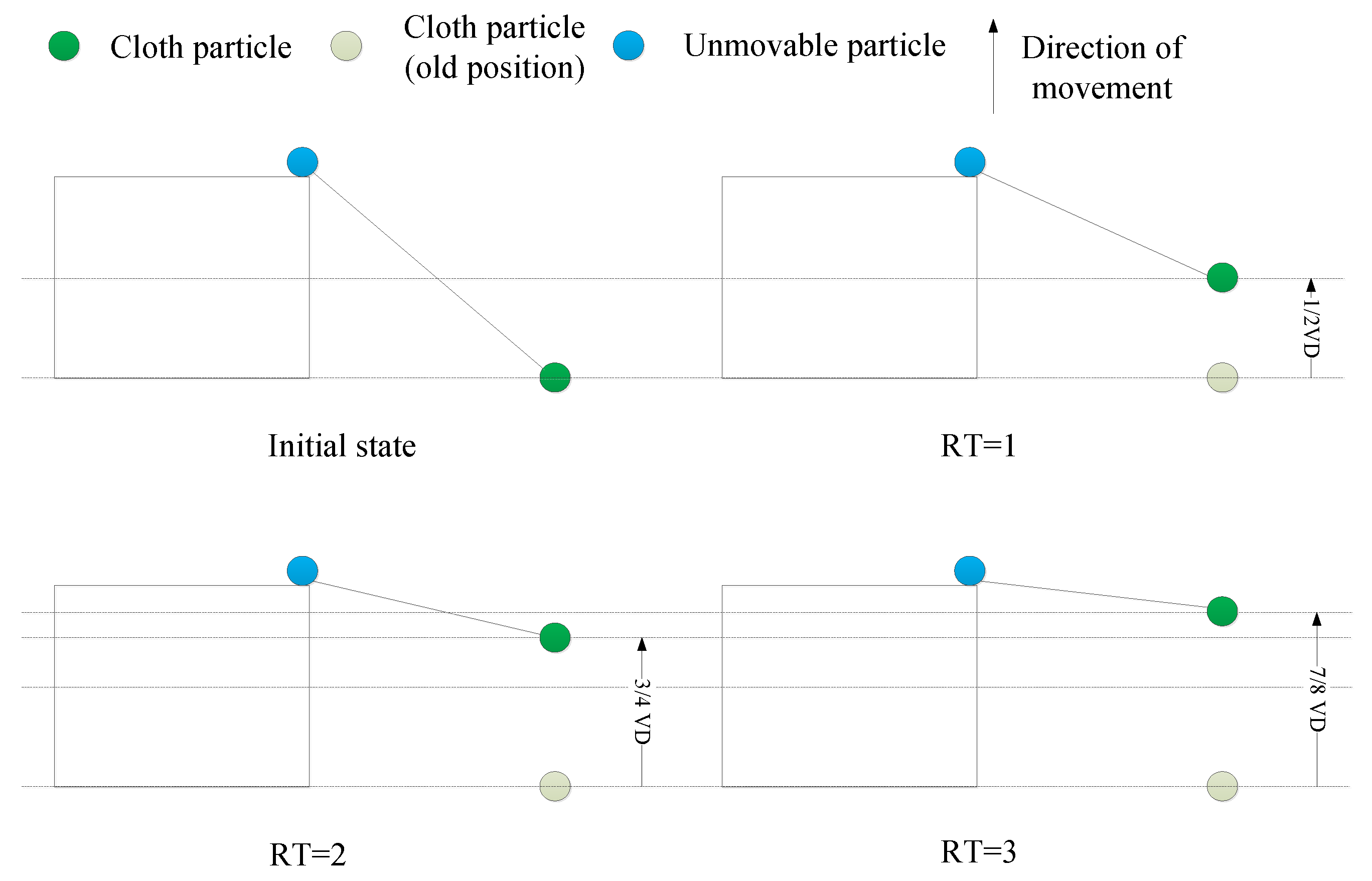
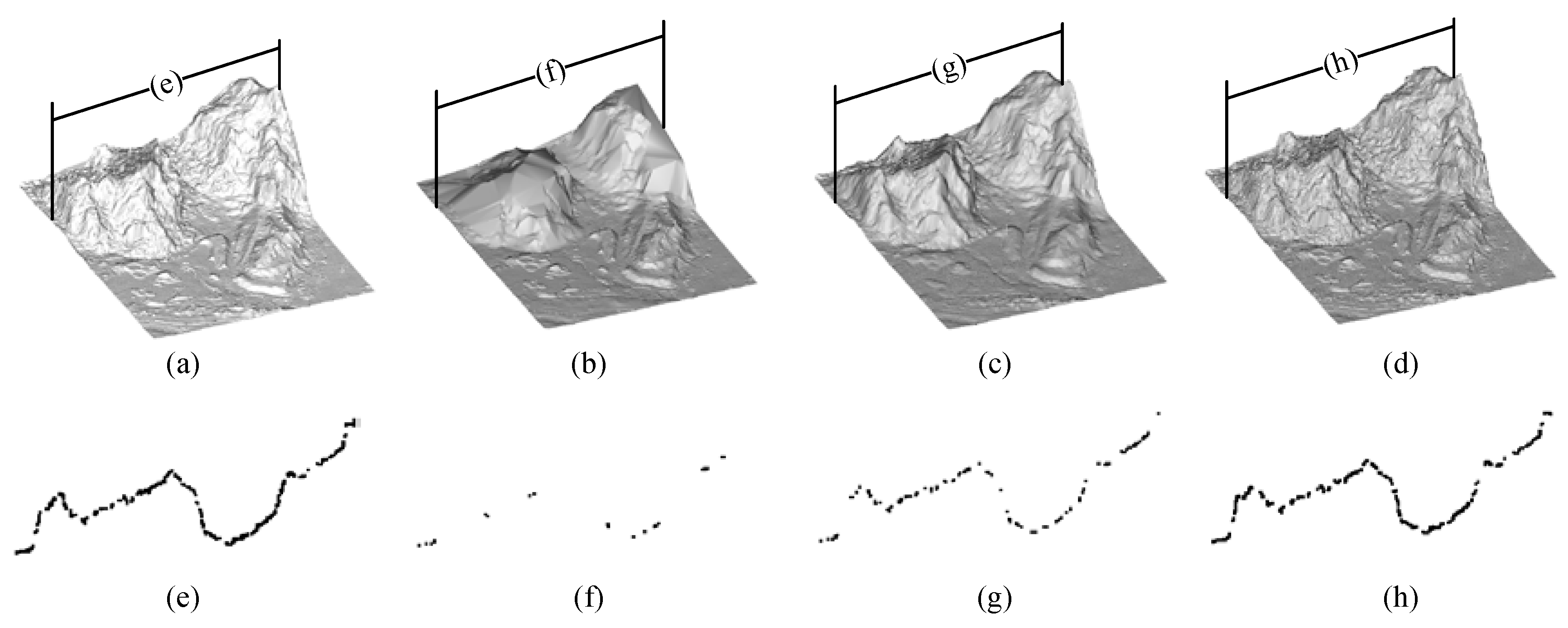
3.1.1. Cloth Simulation
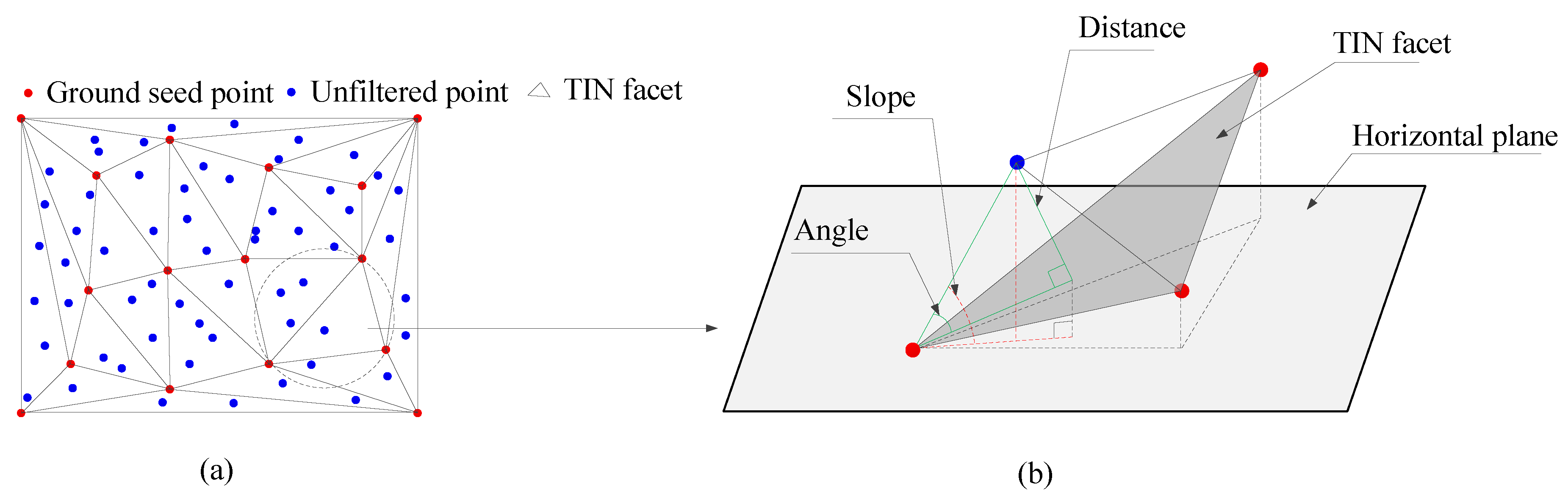
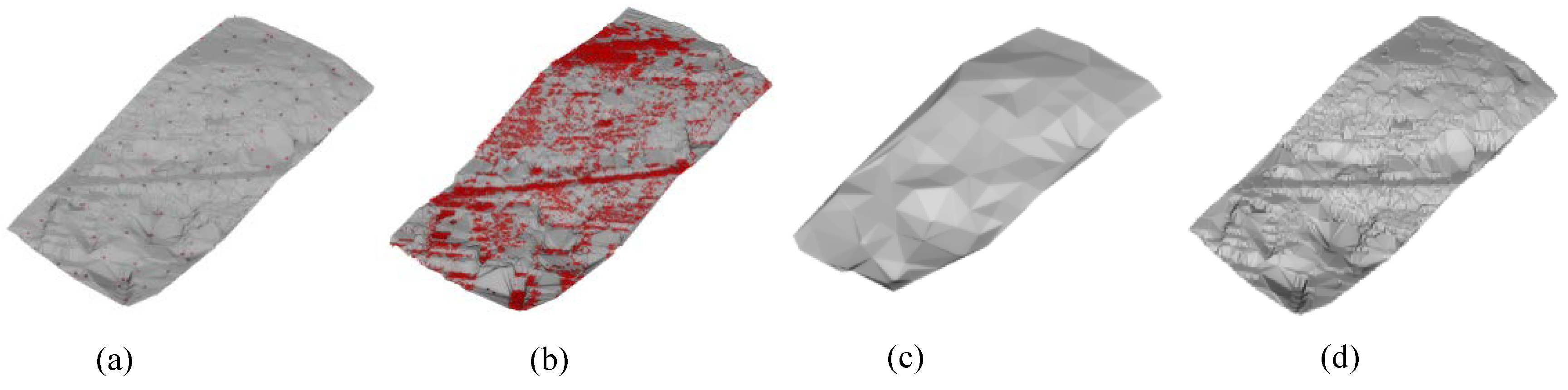
3.1.2. Ground Seed Point Acquisition
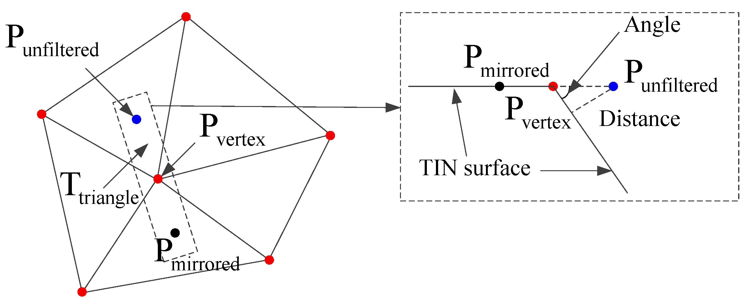
3.1.3. Initial Provisional DTM Construction
3.2. Parameter Threshold Estimation Based on Statistical Analysis
3.3. Refinement of Initial Provisional DTM Based on Progressive TIN Densification
3.4. Accuracy Indexes
4. Experiments
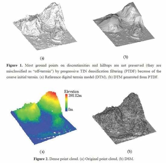
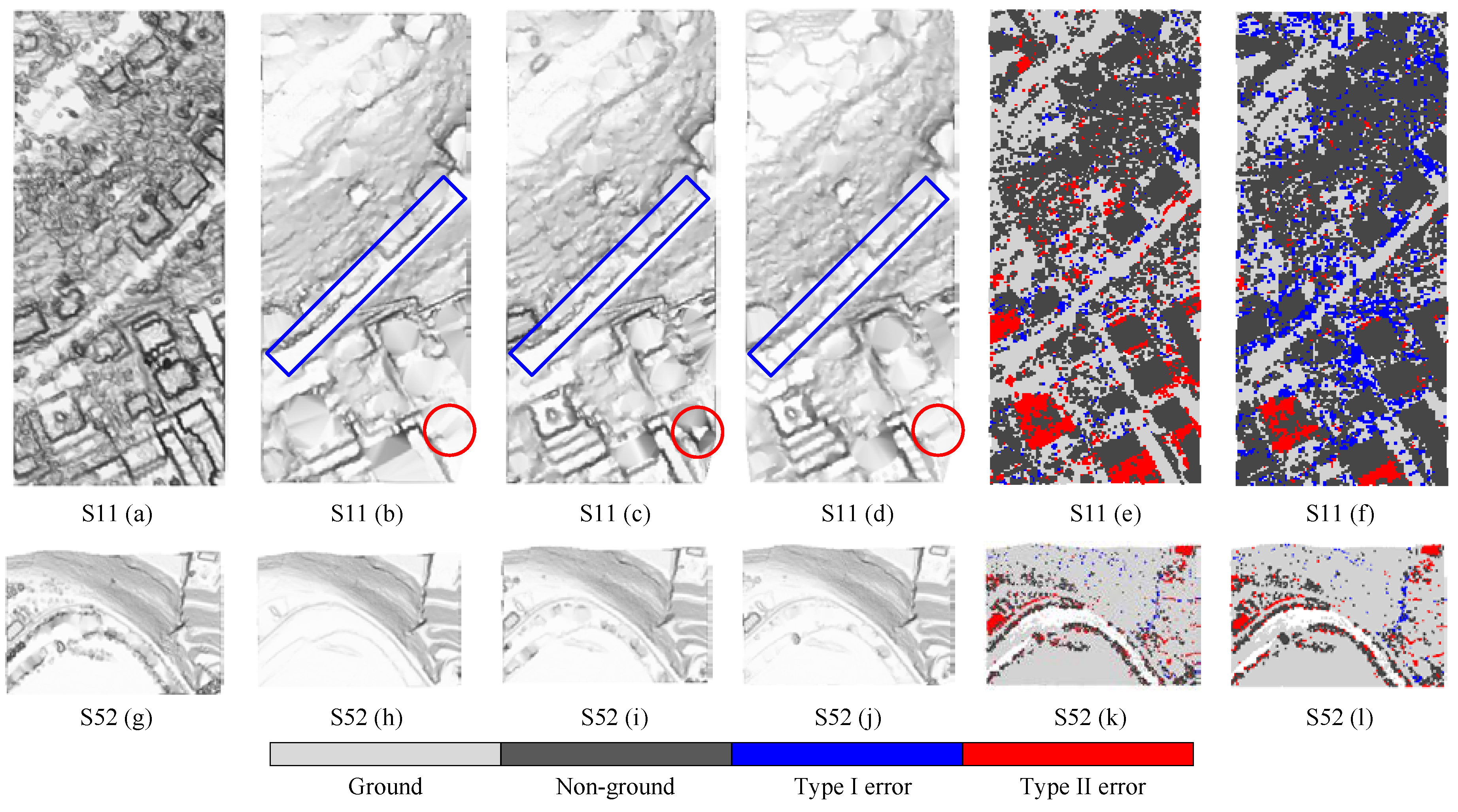
4.1. Testing with ISPRS Dataset
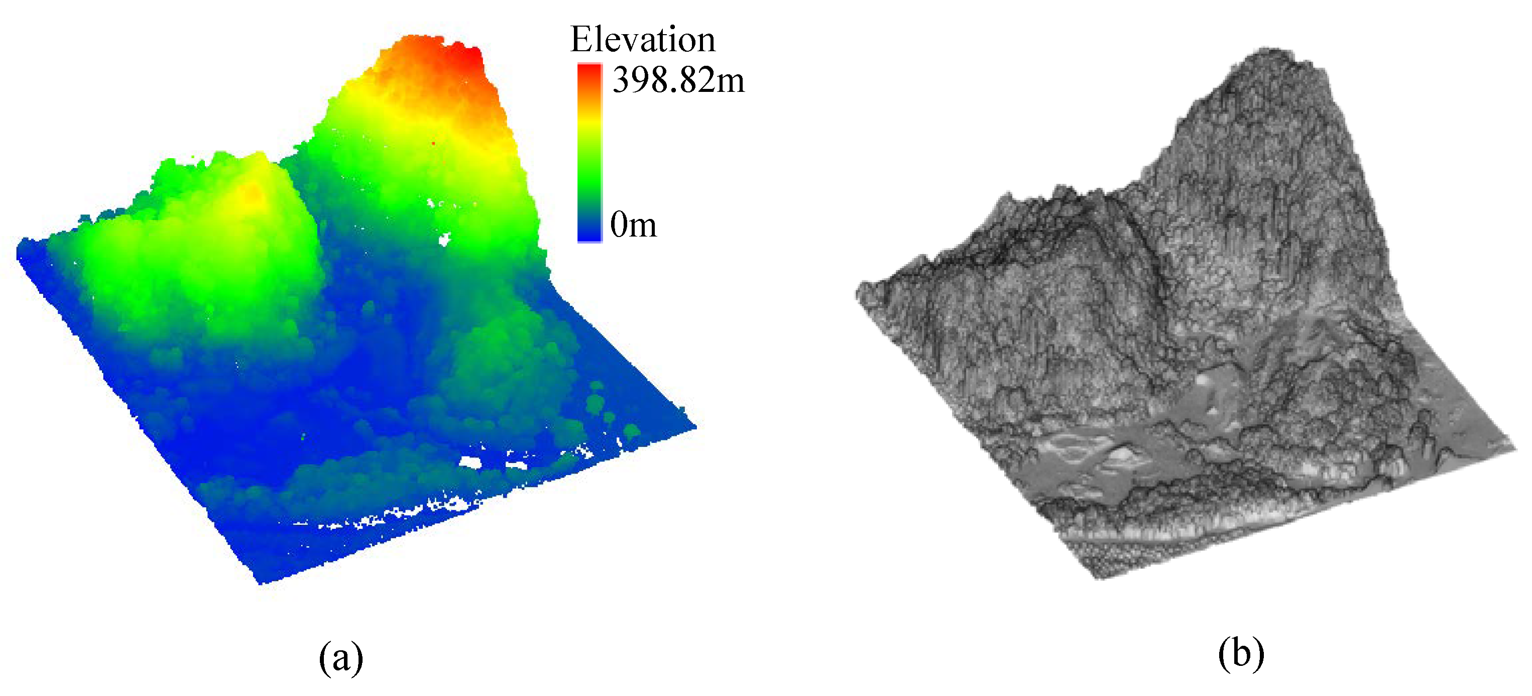
4.2. Testing with Dense Point Cloud
5. Discussion
5.1. Accuracy of Ground Seed Points
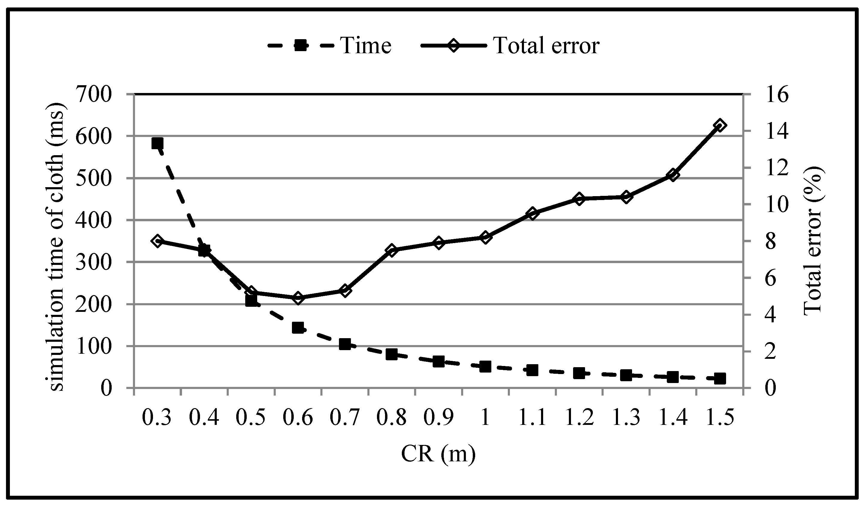
5.2. Parameter Analysis
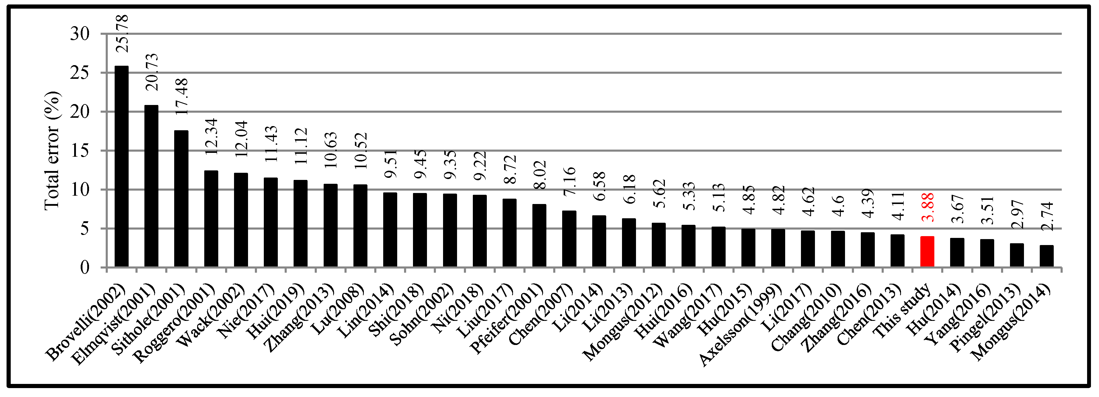
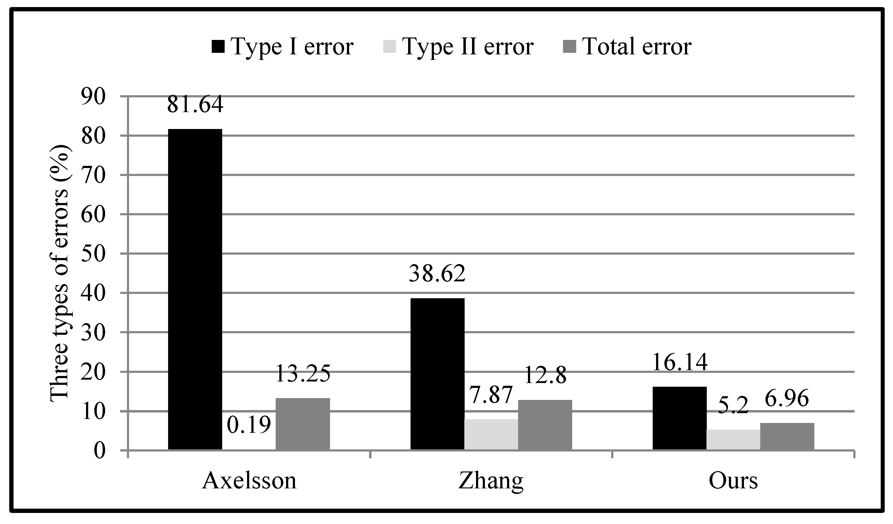
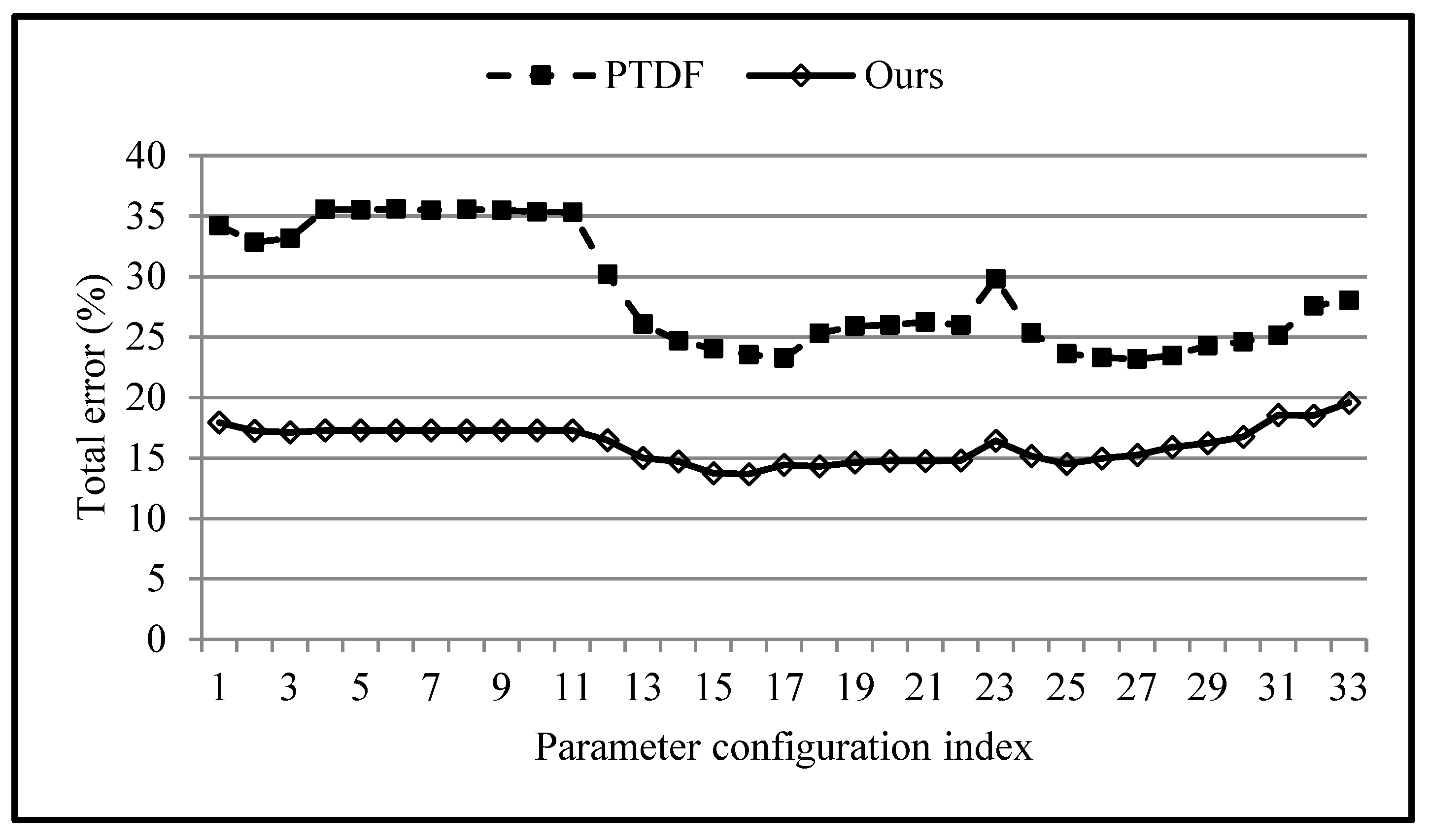
5.3. Four Filters with Higher Accuracy
6. Conclusions
Author Contributions
Funding
Acknowledgments
Conflicts of Interest
References
- Meng, X.; Currit, N.; Zhao, K. Ground filtering algorithms for airborne LiDAR data: A review of critical issues. Remote Sens. 2010, 2, 833–860. [Google Scholar] [CrossRef]
- Sithole, G.; Vosselman, G. Experimental comparison of filter algorithms for bare-Earth extraction from airborne laser scanning point clouds. ISPRS J. Photogramm. Remote Sens. 2004, 59, 85–101. [Google Scholar] [CrossRef]
- Chen, Z.; Gao, B.; Devereux, B. State-of-the-art: DTM generation using airborne LIDAR data. Sensors 2017, 17, 150. [Google Scholar] [CrossRef] [PubMed]
- Liu, X. Airborne LiDAR for DEM generation: Some critical issues. Prog. Phys. Geog. 2008, 32, 31–49. [Google Scholar]
- Guo, Q.; Li, W.; Yu, H.; Alvarez, O. Effects of topographic variability and Lidar sampling density on several DEM interpolation methods. Photogramm. Eng. Remote Sens. 2010, 76, 701–712. [Google Scholar] [CrossRef]
- Hyyppä, J.; Hyyppä, H.; Leckie, D.; Gougeon, F.; Yu, X. Review of methods of small—Footprint airborne laser scanning for extracting forest inventory data in boreal forests. Int. J. Remote Sens. 2008, 29, 37–41. [Google Scholar] [CrossRef]
- Wang, Y.; Hyyppä, J.; Liang, X.; Kaartinen, H.; Yu, X.; Lindberg, E.; Holmgren, J.; Qin, Y.; Mallet, C.; Ferraz, A.; et al. International benchmarking of the individual tree detection methods for modeling 3-D canopy structure for silviculture and forest ecology using airborne laser scanning. IEEE Trans. Geosci. Remote Sens. 2016, 54, 5011–5027. [Google Scholar] [CrossRef]
- Hyyppä, J.; Yu, X.; Hyyppä, H.; Vastaranta, M.; Holopainen, M. Advances in forest inventory using airborne laser scanning. Remote Sens. 2012, 4, 1190–1207. [Google Scholar] [CrossRef]
- Wulder, M.A.; White, J.C.; Nelson, R.F.; Næsset, E.; Ole, H.; Coops, N.C.; Hilker, T.; Bater, C.W.; Gobakken, T. Lidar sampling for large-area forest characterization: A review. Remote Sens. Environ. 2012, 121, 196–209. [Google Scholar] [CrossRef]
- Lim, K.; Treitz, P.; Wulder, M.; St-onge, B.; Flood, M. LiDAR remote sensing of forest structure. Prog. Phys. Geog. 2003, 27, 88–106. [Google Scholar] [CrossRef]
- Drake, J.B.; Dubayah, R.O.; Clark, D.B.; Knox, R.G.; Blair, J.B.; Hofton, M.A.; Chazdon, R.L.; Weishampel, J.F.; Prince, S. Estimation of tropical forest structural characteristics, using large-footprint lidar. Remote Sens. Environ. 2002, 79, 305–319. [Google Scholar] [CrossRef]
- Means, J.E.; Acker, S.A.; Fitt, B.J.; Renslow, M.; Emerson, L.; Hendrix, C.J. Predicting forest stand characteristics with airborne scanning lidar. Photogramm. Eng. Remote Sens. 2000, 66, 1367–1371. [Google Scholar]
- Rottensteiner, F.; Sohn, G.; Gerke, M.; Dirk, J.; Breitkopf, U.; Jung, J. Results of the ISPRS benchmark on urban object detection and 3D building reconstruction. ISPRS J. Photogramm. Remote Sens. 2014, 93, 256–271. [Google Scholar] [CrossRef]
- Wang, R. 3D building modeling using images and LiDAR: A review. Int. J. Image Data Fusion. 2013, 4, 273–292. [Google Scholar] [CrossRef]
- Wang, R.; Peethambaran, J.; Chen, D. LiDAR point clouds to 3-D urban models: A review. IEEE J. Sel. Top. Appl. Earth Obs. Remote Sens. 2018, 11, 606–627. [Google Scholar] [CrossRef]
- Sampath, A.; Shan, J. Segmentation and reconstruction of polyhedral building roofs from aerial Lidar point clouds. IEEE Trans. Geosci. Remote Sens. 2010, 48, 1554–1567. [Google Scholar] [CrossRef]
- Vosselman, G. Slope based filtering of laser altimetry data. Int. Arch. Photogramm. Remote Sens. 2000, 33, 935–942. [Google Scholar]
- Sithole, G. Filtering of laser altimetry data using a slope adaptive filter. Int. Arch. Photogramm. Remote Sens. Spat. Inf. Sci. 2001, 34, 203–210. [Google Scholar]
- Shan, J.; Sampath, A. Urban DEM generation from raw lidar data. Photogramm. Eng. Remote Sens. 2005, 71, 217–226. [Google Scholar] [CrossRef]
- Meng, X.; Wang, L.; Silván-Cárdenas, J.L.; Currit, N. A multi-directional ground filtering algorithm for airborne LIDAR. ISPRS J. Photogramm. Remote Sens. 2009, 64, 117–124. [Google Scholar] [CrossRef]
- Susaki, J. Adaptive slope filtering of airborne lidar data in urban areas for Digital Terrain Model (DTM) generation. Remote Sens. 2012, 4, 1804–1819. [Google Scholar] [CrossRef]
- Keqi, Z.; Shu-Ching, C.; Whitman, D.; Mei-Ling, S.; Jianhua, Y.; Chengcui, Z.; Zhang, K. A progressive morphological filter for removing nonground measurements from airborne LIDAR data. IEEE Trans. Geosci. Remote Sens. 2003, 41, 872–882. [Google Scholar] [CrossRef]
- Chen, Q.; Gong, P.; Baldocchi, D.; Xie, G. Filtering airborne laser scanning data with morphological methods. Photogramm. Eng. Remote Sens. 2007, 73, 175–185. [Google Scholar] [CrossRef]
- Pingel, T.J.; Clarke, K.C.; McBride, W.A. An improved simple morphological filter for the terrain classification of airborne LIDAR data. ISPRS J. Photogramm. Remote Sens. 2013, 77, 21–30. [Google Scholar] [CrossRef]
- Li, Y.; Wu, H.; Xu, H.; An, R.; Xu, J.; He, Q. A gradient-constrained morphological filtering algorithm for airborne LiDAR. Opt. Laser Technol. 2013, 54, 288–296. [Google Scholar] [CrossRef]
- Li, Y.; Yong, B.; Wu, H.; An, R.; Xu, H. An improved Top-Hat filter with sloped brim for extracting ground points from airborne Lidar point clouds. Remote Sens. 2014, 6, 12885–12908. [Google Scholar] [CrossRef]
- Hui, Z.; Hu, Y.; Yevenyo, Y.Z.; Yu, X. An improved morphological algorithm for filtering airborne LiDAR point cloud based on multi-level kriging interpolation. Remote Sens. 2016, 8, 35. [Google Scholar] [CrossRef]
- Kraus, K.; Pfeifer, N. Determination of terrain models in wooded areas with aerial laser scanner data. ISPRS J. Photogramm. Remote Sens. 1998, 53, 193–203. [Google Scholar] [CrossRef]
- Pfeifer, N.; Stadler, P.; Briese, C. Derivation of digital terrain models in the SCOP++ environment. In Proceedings of the OEEPE Workshop on Airborne Laser Scanning and Interferometric SAR for Digital Elevation Models, Stockholm, Sweden, 1–3 March 2001. [Google Scholar]
- Elmqvist, M. Ground surface estimation from airborne laser scanner data using active shape models. In Proceedings of the ISPRS Commission III Symposium, Photogrammetric and Computer Vision, Graz, Austria, 9–13 September 2002; pp. 114–118. [Google Scholar]
- Mongus, D.; Žalik, B. Parameter-free ground filtering of LiDAR data for automatic DTM generation. ISPRS J. Photogramm. Remote Sens. 2012, 67, 1–12. [Google Scholar] [CrossRef]
- Maguya, A.S.; Junttila, V.; Kauranne, T. Adaptive algorithm for large scale dtm interpolation from lidar data for forestry applications in steep forested terrain. ISPRS J. Photogramm. Remote Sens. 2013, 85, 74–83. [Google Scholar] [CrossRef]
- Chen, C.; Li, Y.; Li, W.; Dai, H. A multiresolution hierarchical classification algorithm for filtering airborne LiDAR data. ISPRS J. Photogramm. Remote Sens. 2013, 82, 1–9. [Google Scholar] [CrossRef]
- Hu, H.; Ding, Y.; Zhu, Q.; Wu, B.; Lin, H.; Du, Z.; Zhang, Y.; Zhang, Y. An adaptive surface filter for airborne laser scanning point clouds by means of regularization and bending energy. ISPRS J. Photogramm. Remote Sens. 2014, 92, 98–111. [Google Scholar] [CrossRef]
- Qin, L.; Wu, W.; Tian, Y.; Xu, W. LiDAR filtering of urban areas with region growing based on moving-window weighted iterative least-squares fitting. IEEE Geosci. Remote Sens. Lett. 2017, 14, 841–845. [Google Scholar] [CrossRef]
- Axelsson, P. DEM generation from laser scanner data using adaptive TIN models. Int. Arch. Photogramm. Remote Sens. 2000, 33, 111–118. [Google Scholar]
- Zhang, J.; Lin, X. Filtering airborne LiDAR data by embedding smoothness-constrained segmentation in progressive TIN densification. ISPRS J. Photogramm. Remote Sens. 2013, 81, 44–59. [Google Scholar] [CrossRef]
- Lin, X.; Zhang, J. Segmentation-based filtering of airborne LiDAR point clouds by progressive densification of terrain segments. Remote Sens. 2014, 6, 1294–1326. [Google Scholar] [CrossRef]
- Chen, Q.; Wang, H.; Zhang, H.; Sun, M.; Liu, X. A point cloud filtering approach to generating DTMs for steep mountainous areas and adjacent residential areas. Remote Sens. 2016, 8, 71. [Google Scholar] [CrossRef]
- Zhao, X.; Guo, Q.; Su, Y.; Xue, B. Improved progressive TIN densification filtering algorithm for airborne LiDAR data in forested areas. ISPRS J. Photogramm. Remote Sens. 2016, 117, 79–91. [Google Scholar] [CrossRef]
- Liu, X.; Chen, Y.; Cheng, L.; Yao, M.; Deng, S.; Li, M.; Cai, D. Airborne laser scanning point clouds filtering method based on the construction of virtual ground seed points. Appl. Remote Sens. 2017, 11, 016032. [Google Scholar] [CrossRef]
- Nie, S.; Wang, C.; Dong, P.; Xi, X.; Luo, S.; Qin, H. A revised progressive TIN densification for filtering airborne LiDAR data. Measurement 2017, 104, 70–77. [Google Scholar] [CrossRef]
- Shi, X.; Ma, H.; Chen, Y.; Zhang, L.; Zhou, W. A parameter-free progressive TIN densification filtering algorithm for lidar point clouds. Int. J. Remote Sens. 2018, 39, 6969–6982. [Google Scholar] [CrossRef]
- Zhang, W.; Qi, J.; Wan, P.; Wang, H.; Xie, D.; Wang, X. An Easy-to-Use airborne LiDAR data filtering method based on cloth simulation. Remote Sens. 2016, 8, 501. [Google Scholar] [CrossRef]
- Podobnikar, T.; Vrečko, A. Digital elevation model from the best results of different filtering of a LiDAR point cloud. Trans. GIS. 2012, 16, 603–617. [Google Scholar] [CrossRef]
- Montealegre, A.L.; Lamelas, M.T.; De La Riva, J. A Comparison of open-source LiDAR filtering algorithms in a mediterranean forest environment. IEEE J. Sel. Top. Appl. Earth Obs. Remote Sens. 2015, 8, 4072–4085. [Google Scholar] [CrossRef]
- Yang, B.; Huang, R.; Dong, Z.; Zang, Y.; Li, J. Two-step adaptive extraction method for ground points and breaklines from lidar point clouds. ISPRS J. Photogramm. Remote Sens. 2016, 119, 373–389. [Google Scholar] [CrossRef]
- Serifoglu Yilmaz, C.; Yilmaz, V.; Güngör, O. Investigating the performances of commercial and non-commercial software for ground filtering of UAV-based point clouds. Int. J. Remote Sens. 2018, 39, 5016–5042. [Google Scholar] [CrossRef]
- Wan, P.; Zhang, W.; Skidmore, A.K.; Qi, J.; Jin, X.; Yan, G.; Wang, T. A simple terrain relief index for tuning slope-related parameters of LiDAR ground filtering algorithms. ISPRS J. Photogramm. Remote Sens. 2018, 143, 181–190. [Google Scholar] [CrossRef]
- Kobler, A.; Pfeifer, N.; Ogrinc, P.; Todorovski, L.; Oštir, K.; Džeroski, S. Repetitive interpolation: A robust algorithm for DTM generation from Aerial Laser Scanner Data in forested terrain. Remote Sens. Environ. 2007, 108, 9–23. [Google Scholar] [CrossRef]
- Guan, H.; Li, J.; Yu, Y.; Zhong, L.; Ji, Z. DEM generation from lidar data in wooded mountain areas by cross-section-plane analysis. Int. J. Remote Sens. 2014, 35, 927–948. [Google Scholar] [CrossRef]
- Hodgson, M.E.; Bresnahan, P. Accuracy of Airborne Lidar-Derived Elevation: Empirical Assessment and Error Budget. Photogramm. Eng. Remote Sens. 2004, 70, 331–339. [Google Scholar] [CrossRef]
- Zhao, X.; Su, Y.; Li, W.; Hu, T.; Liu, J.; Guo, Q. A comparison of LiDAR filtering algorithms in vegetated mountain areas. Can. J. Remote Sens. 2018, 44. [Google Scholar] [CrossRef]
- Lu, W.L.; Little, J.J.; Sheffer, A.; Fu, H. Deforestation: Extracting 3D bare-earth surface from airborne LiDAR data. In Proceedings of the 2008 Canadian Conference on Computer and Robot Vision, Windsor, ON, Canada, 28–30 May 2008; pp. 203–210. [Google Scholar]
- Chang, L.; Slatton, K.; Krekeler, C. Bare-earth extraction from airborne LiDAR data based on segmentation modeling and iterative surface corrections. Appl. Remote Sens. 2010, 4, 1–30. [Google Scholar] [CrossRef]
- Mongus, D.; Lukac, N.; Žalik, B. Ground and building extraction from LiDAR data based on differential morphological profiles and locally fitted surfaces. ISPRS J. Photogramm. Remote Sens. 2014, 93, 145–156. [Google Scholar] [CrossRef]
- Hu, X.; Ye, L.; Pang, S.; Shan, J. Semi-global filtering of airborne LiDAR fata for fast extraction of digital terrain models. Remote Sens. 2015, 7, 10996–11015. [Google Scholar] [CrossRef]
- Li, Y.; Yong, B.; van Oosterom, P.; Lemmens, M.; Wu, H.; Ren, L.; Zheng, M.; Zhou, J. Airborne LiDAR data filtering based on geodesic transformations of mathematical morphology. Remote Sens. 2017, 9, 1104. [Google Scholar] [CrossRef]
- Wang, L.; Xu, Y.; Li, Y. Aerial Lidar point cloud voxelization with its 3D ground filtering application. Photogramm. Eng. Remote Sens. 2017, 83, 95–107. [Google Scholar] [CrossRef]
- Ni, H.; Lin, X.; Zhang, J.; Chen, D.; Peethambaran, J. Joint clusters and iterative graph cuts for ALS point cloud filtering. IEEE J. Sel. Top. Appl. Earth Obs. Remote Sens. 2018, 11, 990–1004. [Google Scholar] [CrossRef]
- Hui, Z.; Li, D.; Jin, S.; Ziggah, Y.; Wang, L.; Hu, Y. Automatic DTM extraction from airborne LiDAR based on expectationmaximization. Opt. Laser Technol. 2019, 112, 43–55. [Google Scholar] [CrossRef]
- Khosravipour, A.; Skidmore, A.K.; Isenburg, M.; Wang, T.; Hussin, Y.A. Generating pit-free canopy height models from airborne lidar. Photogramm. Eng. Remote Sens. 2014, 80, 863–872. [Google Scholar] [CrossRef]
- Zhang, K.; Whitman, D. Comparison of three algorithms for filtering airborne LiDAR data. Photogramm. Eng. Remote Sens. 2005, 71, 313–324. [Google Scholar] [CrossRef]


| Environment | Site | Sample | Features | Reference (Points) | |
|---|---|---|---|---|---|
| Ground | Non-Ground | ||||
| Urban | 1 | S11 | Mixture of vegetation and buildings on hillside | 21,786 | 16,224 |
| S12 | Mixture of vegetation and buildings | 26,691 | 25,428 | ||
| 2 | S21 | Road with bridge | 10,085 | 2875 | |
| S22 | Irregularly shaped buildings and bridge | 22,504 | 10,202 | ||
| S23 | Large, irregularly shaped buildings | 13,223 | 11,872 | ||
| S24 | Steep slopes | 5434 | 2058 | ||
| 3 | S31 | Complex buildings | 15,556 | 13,306 | |
| 4 | S41 | Data gaps, irregularly shaped buildings | 5602 | 5629 | |
| S42 | Railway station with trains | 12,443 | 30,027 | ||
| Rural | 5 | S51 | Vegetation on hillside | 13,950 | 3895 |
| S52 | Steep, terraced slopes | 20,112 | 2362 | ||
| S53 | Steep, terraced slopes | 32,989 | 1389 | ||
| S54 | Dense buildings | 3983 | 4625 | ||
| 6 | S61 | Data gaps, discontinuity | 33,854 | 1206 | |
| 7 | S71 | Underpass and bridge | 13,875 | 1770 | |
| Samples | Zhang and Lin | Nie et al. | The Proposed Algorithm | |||||||||
|---|---|---|---|---|---|---|---|---|---|---|---|---|
| c(m) | d(m) | c(m) | d(m) | c(m) | d(m) | |||||||
| S11 | 20 | 6 | 1.4 | 80 | 20 | 15 | 1.4 | 80 | 1 | 23.37 | >15 | 88.96 |
| S12 | 20 | 6 | 1.4 | 80 | 20 | 15 | 1.4 | 80 | 1 | 32.68 | >15 | 85.04 |
| S21 | 60 | 6 | 1.4 | 88 | 60 | 15 | 1.4 | 88 | 1 | 23.12 | >15 | 62.71 |
| S22 | 60 | 6 | 1.4 | 88 | 60 | 15 | 1.4 | 88 | 1 | 18.21 | >15 | 88.26 |
| S23 | 60 | 6 | 1.4 | 88 | 60 | 15 | 1.4 | 88 | 1 | 28.21 | >15 | 85.63 |
| S24 | 60 | 6 | 1.4 | 88 | 60 | 15 | 1.4 | 88 | 1 | 25.6 | >15 | 63.37 |
| S31 | 35 | 6 | 1.4 | 88 | 35 | 15 | 1.4 | 88 | 1 | 9.33 | >15 | 84.71 |
| S41 | 60 | 6 | 1.4 | 88 | 60 | 15 | 1.4 | 88 | 1 | 15.62 | >15 | 62.23 |
| S42 | 60 | 6 | 1.4 | 88 | 60 | 15 | 1.4 | 88 | 1 | 16.37 | >15 | 70.76 |
| S51 | 10 | 6 | 1 | 70 | 10 | 15 | 1 | 70 | 1 | 18.75 | >15 | 82.42 |
| S52 | 10 | 6 | 1 | 70 | 10 | 15 | 1 | 70 | 1 | 22.02 | >15 | 86.37 |
| S53 | 10 | 6 | 1 | 70 | 10 | 15 | 1 | 70 | 1 | 27.96 | >15 | 85.92 |
| S54 | 10 | 6 | 1 | 70 | 10 | 15 | 1 | 70 | 1 | 16.06 | >15 | 59.33 |
| S61 | 40 | 6 | 1.4 | 70 | 40 | 15 | 1.4 | 70 | 1 | 20.64 | >15 | 80.97 |
| S71 | 20 | 6 | 1.4 | 70 | 20 | 15 | 1.4 | 70 | 1 | 16.38 | >15 | 62.32 |
| Samples | Zhang and Lin | Lin and Zhang | Nie et al. | Shi et al. | Ours |
|---|---|---|---|---|---|
| S11 | 18.49 | 19.5 | 18.79 | 11.12 | 16.24 |
| S12 | 5.92 | 4.78 | 6.62 | 7.17 | 8.85 |
| S21 | 4.95 | 6.08 | 5.60 | 6.58 | 14.18 |
| S22 | 14.18 | 9.24 | 14.89 | 14.02 | 4.25 |
| S23 | 12.06 | 14.43 | 18.08 | 17.43 | 8.52 |
| S24 | 20.26 | 5.28 | 24.57 | 13.06 | 15.59 |
| S31 | 2.32 | 1.61 | 2.14 | 3.13 | 7.28 |
| S41 | 20.44 | 32 | 27.13 | 10.06 | 13.04 |
| S42 | 3.94 | 5.95 | 2.42 | 1.91 | 4.75 |
| S51 | 5.31 | 4.09 | 2.85 | 12.69 | 3.51 |
| S52 | 12.98 | 7.56 | 14.43 | 16.67 | 4.65 |
| S53 | 5.58 | 9.9 | 19.37 | 9.77 | 3.95 |
| S54 | 6.4 | 10.72 | 4 | 4.99 | 2.58 |
| S61 | 16.13 | 6.27 | 6.89 | 7.51 | 0.86 |
| S71 | 10.44 | 5.22 | 3.68 | 5.68 | 2.03 |
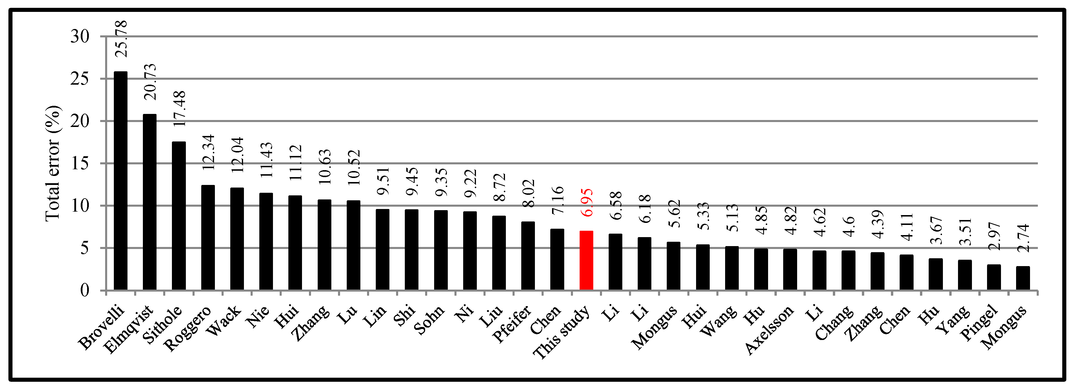
| Avg. | 10.63 | 9.51 | 11.43 | 9.45 | 6.95 |
| Samples | Zhang and Lin | Lin and Zhang | Nie et al. | Shi et al. | Ours | |||||
| I | II | I | II | I | II | I | II | I | II | |
| S11 | 25.67 | 8.84 | 26.28 | 10.4 | 37.24 | 1.35 | 14.74 | 6.07 | 7.51 | 27.98 |
| S12 | 8.13 | 3.61 | 6.56 | 3.31 | 11.86 | 1.05 | 11.86 | 1.93 | 4.68 | 13.21 |
| S21 | 1.17 | 18.23 | 0.85 | 24.45 | 6.2 | 4.49 | 7.54 | 3.18 | 16.27 | 6.87 |
| S22 | 19.05 | 3.44 | 6.43 | 15.44 | 20.82 | 3.6 | 19.44 | 2.15 | 2.22 | 8.73 |
| S23 | 19.25 | 4.05 | 23.21 | 4.64 | 35.63 | 1.6 | 29.69 | 3.89 | 3.48 | 14.13 |
| S24 | 22.86 | 13.41 | 3.99 | 8.7 | 32.58 | 15.42 | 15.86 | 5.63 | 3.13 | 48.49 |
| S31 | 2.1 | 2.59 | 0.54 | 2.59 | 2.02 | 2.41 | 4.61 | 1.43 | 12.74 | 0.91 |
| S41 | 39.54 | 1.44 | 62.22 | 1.92 | 52.03 | 0.32 | 17.92 | 2.33 | 25.56 | 0.35 |
| S42 | 9.72 | 1.55 | 19.02 | 0.54 | 6.69 | 1.26 | 3.88 | 1.1 | 9.71 | 2.71 |
| S51 | 2.05 | 16.97 | 2.22 | 10.81 | 2.9 | 2.77 | 15.14 | 3.79 | 0.07 | 15.81 |
| S52 | 12.53 | 16.77 | 6.46 | 16.89 | 16.14 | 2.96 | 17.52 | 9.31 | 0.98 | 35.9 |
| S53 | 4.25 | 37.22 | 9.62 | 16.41 | 20.22 | 0.72 | 10.11 | 1.77 | 2.72 | 33.05 |
| S54 | 3.59 | 8.82 | 3.16 | 17.23 | 6.76 | 1.78 | 8.65 | 1.87 | 1.16 | 3.81 |
| S61 | 16.62 | 2.49 | 6.26 | 6.55 | 8.17 | 2.07 | 7.75 | 0.84 | 0.39 | 13.93 |
| S71 | 10.07 | 13.39 | 2.62 | 25.65 | 5.24 | 0.79 | 6 | 3.18 | 0.28 | 15.71 |
| Avg. | 13.11 | 10.19 | 11.96 | 11.06 | 17.63 | 2.84 | 12.71 | 3.23 | 4.6 | 11.42 |
| Samples | PTDF (Points) | Ours (Points) | OP (%) |
|---|---|---|---|
| S11 | 116 | 12,863 | 94.75 |
| S12 | 158 | 12,135 | 98.95 |
| S21 | 10 | 4600 | 99.7 |
| S22 | 20 | 9973 | 99.38 |
| S23 | 16 | 6391 | 98.18 |
| S24 | 10 | 2554 | 98.08 |
| S31 | 29 | 7687 | 99.32 |
| S41 | 10 | 2310 | 99.65 |
| S42 | 20 | 6377 | 94.65 |
| S51 | 1008 | 10,247 | 97.3 |
| S52 | 1329 | 14,942 | 98.02 |
| S53 | 1935 | 23,544 | 99.57 |
| S54 | 517 | 2727 | 99.12 |
| S61 | 146 | 28,112 | 99.8 |
| S71 | 224 | 11,062 | 99.39 |
| Avg. | 369.87 | 10,368.27 | 98.39 |
© 2019 by the authors. Licensee MDPI, Basel, Switzerland. This article is an open access article distributed under the terms and conditions of the Creative Commons Attribution (CC BY) license (http://creativecommons.org/licenses/by/4.0/).
Share and Cite
Cai, S.; Zhang, W.; Liang, X.; Wan, P.; Qi, J.; Yu, S.; Yan, G.; Shao, J. Filtering Airborne LiDAR Data Through Complementary Cloth Simulation and Progressive TIN Densification Filters. Remote Sens. 2019, 11, 1037. https://doi.org/10.3390/rs11091037
Cai S, Zhang W, Liang X, Wan P, Qi J, Yu S, Yan G, Shao J. Filtering Airborne LiDAR Data Through Complementary Cloth Simulation and Progressive TIN Densification Filters. Remote Sensing. 2019; 11(9):1037. https://doi.org/10.3390/rs11091037
Chicago/Turabian StyleCai, Shangshu, Wuming Zhang, Xinlian Liang, Peng Wan, Jianbo Qi, Sisi Yu, Guangjian Yan, and Jie Shao. 2019. "Filtering Airborne LiDAR Data Through Complementary Cloth Simulation and Progressive TIN Densification Filters" Remote Sensing 11, no. 9: 1037. https://doi.org/10.3390/rs11091037
APA StyleCai, S., Zhang, W., Liang, X., Wan, P., Qi, J., Yu, S., Yan, G., & Shao, J. (2019). Filtering Airborne LiDAR Data Through Complementary Cloth Simulation and Progressive TIN Densification Filters. Remote Sensing, 11(9), 1037. https://doi.org/10.3390/rs11091037