The Influence of Different Modelling Factors on Global Temperature and Pressure Models and Their Performance in Different Zenith Hydrostatic Delay (ZHD) Models

Abstract

Surface temperature and pressure are indispensable variables in Global Navigation Satellite System (GNSS) meteorology. The lack of meteorological observations located at or near the GNSS sites is a big challenge for the calculation of accurate zenith hydrostatic delay (ZHD). Therefore, various empirical models with different model forms were established to provide temperature and pressure values. In this study, the influence of different modelling factors, including model forms, temporal resolution of the data sources, and the spatial resolution of the data sources, is evaluated and the temperature and pressure model with the best performance is developed. On the basis of the meteorological parameters estimated by the above model, we analyzed the global performance of the three most commonly used ZHD models, that is, the Saastamoinen, Hopfield, and Black models. The numerical results show that the model with the idea of time-segmented modelling performs best, of which the global mean root mean square (RMS), mean absolute error (MAE), and standard deviation (SD) are 7.87/6.33/7.17 hPa and 2.95/2.31/2.79 K for pressure and temperature, respectively, using the data sources with temporal resolution of 2 h and spatial resolution of 2.5° × 2° in the reanalysis data comparison. In comparison with the radiosonde data, the mean RMS/MAE/SD are 7.02/5.24/6.46 hPa and 4.05/3.17/3.86 K for pressure and temperature, respectively. The Saastamoinen model with a global mean bias/RMS of 1.01/16.9 mm achieved the best ZHD estimated values compared with the other two ZHD models.

1. Introduction

The tropospheric delay of incoming signals remains one of the major influencing factors on the accuracy of Global Navigation Satellite System (GNSS) observations [1,2,3]. A common approach to treating the tropospheric delay is to map the delay into the zenith direction (zenith tropospheric delay, ZTD) through mapping functions, which contains the hydrostatic (zenith hydrostatic delay, ZHD) and wet (zenith wet delay, ZWD) terms. In the high-accuracy geodetic data processing, accurate a priori ZHD is usually needed [4,5]. In addition, accurate ZHD is a prerequisite for obtaining water vapor information in GNSS meteorology, as ZWD is achieved by subtracting ZHD from ZTD [6,7,8,9,10,11].

ZHD can be derived with millimeter-level accuracy from meteorological parameters and position at an observation station using a model, such as the Saastamoinen, Hopfield, and Black models [12,13,14]. However, most GNSS sites are not equipped with meteorological sensors, and there are often no collocated weather stations available for those GNSS sites. Thus, a standard model for providing precise and unbiased global pressure and temperature values is often used, for example, the global pressure and temperature (GPT) series models, TropGrid2 model, and the improved tropospheric grid (ITG) model [15,16,17,18,19].

The GPT model is proposed by Boehm et al. [15], which is developed from three-year European Center for Medium-Range Weather Forecasts (ECMWF) reanalysis (ERA)-40 products, and provides temperature and pressure based on spherical harmonics up to degree and order 9, leading to coarse horizontal resolution of about 20º. A more precise ECMWF ERA-interim product was applied by Lagler et al. to establish the GPT2 model [16,20], in which the semi-annual harmonics was incorporated to better account for regions where very rainy periods or very dry periods dominate, making it an improved model to provide meteorological parameters resting upon a global 5º grid of mean values, annual, and semi-annual variations. TropGrid2 is based on more than nine years of global data assimilation system (GDAS) 3D weather fields, which takes diurnal variations into consideration, but ignores the influence of the semi-annual variations [18]. The ITG model improved the performance of estimating meteorological parameters by considering the annual, semi-annual, and diurnal variations [19].

However, the model form determination, as well as the data source used for the model on a global scale, is a key issue for the construction of the empirical model [21]. Different model forms have different considerations. For example, some models only account for the annual and semi-annual cycles [15,16,17], some models add the diurnal cycles [18], and some models even consider the seasonal variations of diurnal amplitudes and diurnal phases [19]. We compared the different model forms and selected the most suitable one in this paper. Moreover, the latest climate reanalysis (ERA5) produced by ECMWF provides hourly meteorological parameters for the first time, making it possible to perform the analysis of accuracy using data sources with different temporal resolutions. In addition, the results with different spatial resolutions of data sources were compared in the form of a grid.

On the basis of the above comparisons, the temperature and pressure model with the best performance is selected to compute ZHD using different ZHD models, for example, the Saastamoinen, Hopfield, and Black models, which are proved to achieve ZHD values with high accuracy using measured meteorological parameters [8,22,23,24,25,26,27,28]. However, the accuracies of the temperature and pressure estimated by the models vary from area to area, which may result in different performances of the ZHD models using the estimated meteorological parameters. In this paper, the accuracy of three most commonly used ZHD models, which were tested by measured parameters in previous articles, are explored in the case of estimated parameters.

The remainder of this paper is organized as follows. Section 2 introduces the data sources and model forms, while Section 3 presents the evaluation of the models from three aspects, that is, the model forms, the temporal resolution of the data sources, and the spatial resolution of the data sources. Section 4 discusses the accuracy of the three ZHD models using the estimated meteorological parameters, and Section 5 presents the conclusions.

2. Materials and Methods

Owing to the advantages of spatial integrity, temporal continuity, and high accuracy, meteorological reanalysis products, such as ECMWF and National Centers for Environmental Prediction (NCEP), are very suitable for constructing empirical pressure and temperature models. They can provide comprehensive global records of historical atmosphere status spanning an extended period, using a single consistent assimilation scheme throughout. The accuracy of NCEP and ECMWF has been compared by several studies [29], and it is shown that products of ECMWF are more accurate [30,31,32,33]. Thus, in this paper, ERA5 surface products will be utilized for modelling pressure and temperature, while ERA5 pressure level products will be used for modelling temperature lapse rate and specific humidity, which are necessary parameters for temperature and pressure computation.

For pressure and temperature, only annual and semi-annual cycles were considered in most of the commonly used models. The ITG model adopted 15 parameters, considering the diurnal cycles and even the seasonal variations of diurnal amplitudes and diurnal phases. Theoretically, the increase of parameters in one model is beneficial to improve the accuracy of the model, but it also increases the complexity, which is not conductive to its applications. In this work, the performance of four traditional model forms in constructing temperature and pressure models was explored comprehensively, and a type of model based on the idea of time-segmented modelling was compared with the traditional ones. The most suitable model form was then selected from the following five kinds of model forms.

The first form, as Equation (1), which only considers the annual and semi-annual cycles, is regarded as Model #1. In this model form, $a$ are the estimated meteorological parameters; $a_0$ are the mean values; $a_1$ and $a_2$ are the amplitudes of annual and semi-annual periodicity, respectively; $c_1$ and $c_2$ are the initial phase of annual and semi-annual periodicity, respectively; and doy is the day of the year.

$$a=a_0+a_1·\cos \left(\frac{doy-c_1}{365.25}·2\pi \right)+a_2·\cos \left(\frac{doy-c_2}{365.25}·4\pi \right)$$

(1)

When the basic form of diurnal periodicity is considered, that is, the fixed amplitude $a_3$ and diurnal phase $c_3$ are added, the model form as Equation (2) with seven coefficients is regarded as Model #2. hod refers to the hour of the day.

$$a=a_0+a_1·\cos \left(\frac{doy-c_1}{365.25}·2\pi \right)+a_2·\cos \left(\frac{doy-c_2}{365.25}·4\pi \right)+a_3·\cos \left(\frac{hod-c_3}{24}·2\pi \right)$$

(2)

The amplitude and initial phase of diurnal variation can also be estimated as periodic functions with annual and semi-annual periodicity. The coefficients $a_3$ and $c_3$ can be further expanded and expressed as a function of time as follows. Model #3 contains 11 coefficients, and only considers the amplitude of diurnal variation as periodic functions, while Model #4 contains 15 coefficients, and takes $a_3$ and $c_3$ as a function of time.

$$a_3=A_0+A_1·\cos \left(\frac{doy-C_1}{365.25}2\pi \right)+A_2·\cos \left(\frac{doy-C_2}{365.25}4\pi \right)$$

(3)

$$c_3=A_{c0}+A_{c1}·\cos \left(\frac{doy-C_{c1}}{365.25}2\pi \right)+A_{c2}·\cos \left(\frac{doy-C_{c2}}{365.25}4\pi \right)$$

(4)

On the basis of the idea of time-segmented modelling, we can establish models using data at different UTC times separately, for example, only the data of UTC 0:00 are selected to build a model for UTC 0:00 and the data of other time are used for models of other time. The specific choice of which time to model is determined by the temporal resolution of the source data. Thus, Model #5 is as follows:

$$\{\begin{array}{c}{a}^{ho{d}_1}=a_0^{ho{d}_1}+a_1^{ho{d}_1}\cos \left(\frac{doy-c_1^{ho{d}_1}}{365.25}2\pi \right)+a_2^{ho{d}_1}\cos \left(\frac{doy-c_2^{ho{d}_1}}{365.25}4\pi \right)\\ a^{ho{d}_2}=a_0^{ho{d}_2}+a_1^{ho{d}_2}\cos \left(\frac{doy-c_1^{ho{d}_2}}{365.25}2\pi \right)+a_2^{ho{d}_2}\cos \left(\frac{doy-c_2^{ho{d}_2}}{365.25}4\pi \right)\\ ⋮\\ a^{ho{d}_n}=a_0^{ho{d}_n}+a_1^{ho{d}_n}\cos \left(\frac{doy-c_1^{ho{d}_n}}{365.25}2\pi \right)+a_2^{ho{d}_n}\cos \left(\frac{doy-c_2^{ho{d}_n}}{365.25}4\pi \right)\end{array},$$

(5)

where $N$ refers to the number of modelling epochs we choose. $ho{d}_1$, $ho{d}_2$, $ho{d}_3$, $\cdots$ and $ho{d}_n$ represent the different UTC epochs. To calculate the meteorological parameters at a certain epoch, the 10 adjacent epochs near the time to be calculated were searched first, and the parameters of the 10 epochs could be estimated by Equation (5). Then, the value of the time to be calculated can be achieved by interpolating using the Lagrange polynomial. This model can well express the annual, semi-annual, and diurnal cycle characteristics of the meteorological parameters.

3. Evaluation of the Empirical Models

In this section, the influence of different factors on the modelling of meteorological parameters is analyzed, for example, the influence of model forms, the temporal resolution of the data sources, and the spatial resolution of the data sources.

3.1. Influence of Model Forms

The six years (2011–2016) of global surface products for temperature and pressure, as well as the six years (2011–2016) of global profiles containing 37 levels for temperature, specific humidity, and geopotential, were retrieved from ERA5, which was discretized at 5° from 90°N to 90°S for latitude and from 180°W to 180°E for longitude. The five years (2011–2015) of retrieved data with 6 h temporal resolution are used to establish the five kinds of models in Section 2, one year (2016) of the data with 1 h temporal resolution is used to evaluate the accuracy of the models.

The root mean squares (RMSs) of the four meteorological parameters calculated by different models are counted and grouped into different latitude bins, separated by a 5° interval from 90°N to 90°S. To better show the difference between models, the differences of the RMS of four meteorological values with respect to the RMS of Model #1 were shown in Figure 1. From the bottom panel, it is clear that the models considering the diurnal cycles (Model #2–#5) have no obvious improvement in accuracy of temperature lapse rate and specific humidity calculation compared with Model #1, which only considers the annual and semi-annual cycles. This indicates that the diurnal cycle can be ignored when modelling temperature lapse rate and specific humidity. From the upper panel, the improvement to temperature and pressure of models considering the diurnal cycles can be observed, especially in the low latitudes. It is observed that Model #4 performs worse than the other three models, and the improvement of Model #5 is larger than the other three models, especially in the low latitudes for pressure.

To further show the different performance of the models with and without considering the daily cycle in different regions, we selected 21 grid points distributed at longitude of 90°W, 0°, and 90°E and latitude of 90°N, 60°N, 30°N, 0°, 30°S, 60°S, and 90°S. The time-series of true temperature extracted from the reanalysis data of 2016, as well as the time-series of estimated temperature by the five models, is depicted in Figure 2. The yellow line representing Model #1 is a smooth curve in all regions, it does not present the fluctuations in temperature well. When the diurnal cycle is considered in the model, the estimated temperature can well describe the daily change of true temperature, especially in the low latitudes. In this stage, we cannot determine the best model to perform the diurnal cycle. The figure for pressure is similar to Figure 2 and is not repeated here.

Table 1. The root mean square (RMS), mean absolute error (MAE), and standard deviation (SD) of the differences for four meteorological parameters calculated by different models, validated by the data of 2016.

	Temperature (K)			Pressure (hPa)			Temperature Lapse Rate (K/km)			Specific Humidity (g/kg)
	RMS	MAE	SD	RMS	MAE	SD	RMS	MAE	SD	RMS	MAE	SD
Model #1	3.22	2.51	3.10	7.57	6.01	7.42	0.44	0.35	0.43	1.28	1.01	1.24
Model #2	2.98	2.30	2.86	7.45	5.89	7.35	0.44	0.35	0.43	1.28	1.00	1.23
Model #3	2.96	2.29	2.84	7.45	5.89	7.35	0.44	0.35	0.43	1.27	1.00	1.23
Model #4	3.05	2.35	2.92	7.46	5.90	7.35	0.44	0.35	0.43	1.27	1.00	1.23
Model #5	2.96	2.28	2.83	7.42	5.86	7.31	0.44	0.35	0.43	1.27	1.00	1.23

lists the global mean RMS, mean absolute error (MAE), and standard deviation (SD) of differences for four meteorological parameters calculated by different models. For temperature lapse rate and specific humidity, the accuracy of the five kinds of models is comparable and almost unchanged, which is consistent with the result of Figure 1. This illustrates that the time-series of the two meteorological parameters do not contain obvious diurnal cycles. Model #1, only considering the annual and semi-annual cycles, is sufficient to describe the change of these two meteorological parameters. For temperature and pressure, the RMS, MAE, and SD of the models considering the daily cycle are improved in different degrees compared with Model #1. We can find that the RMS/MAE/SD of temperature decrease from 3.22/2.51/3.10 K to 2.98/2.30/2.86 K and then to 2.96/2.29/2.84 K using Model #1, Model #2, and Model #3, respectively, but the accuracy of Model #4 is not improved and worse than that of Model #2. This phenomenon also occurs in the case of pressure validation. The performance of the four traditional models implies that the adoption of sophisticated models (multiple coefficients in one model) does not necessarily improve the accuracy of the temperature and pressure. It is observed that the statistical results achieved by Model #5 are slightly better than those of the others, which indicates the advantages of the time-segmented modelling. Note that the time-segmented model is different from the four traditional models, and does not complicate the model of each epoch.

The empirical distribution functions of the RMS, MAE, and SD of differences for temperature calculated by different models are plotted in Figure 3, in which colors represent different models indicating the percentage of each range of the RMS, MAE, and SD. We can see that the yellow lines representing Model #1 perform worse than the other models in RMS, MAE, and SD. The percentage of RMS/MAE/SD smaller than 5 K is 77%/94%/81% for Model #1; this percentage becomes 82%/95%/84% for Model #4, which has the smallest improvement. Model #5, considering the daily cycle, achieves slightly better results, with a percentage of 85%/97%/86%, than the other two models.

3.2. Influence of Temporal Resolution

The ERA5 reanalysis products provide hourly meteorological data, which makes it possible to analyze the influence of temporal resolution of data sources on pressure and temperature. Apart from the data sources with 6 h temporal resolution used in previous section, the five years’ data from 2011 to 2015 with 3 h and 2 h temporal resolution are selected to establish the meteorological model. In each model, 5° × 5° is selected as the spatial resolution. The meteorological parameters of 2016 with 1 h temporal resolution are regarded as true value for validation.

The global mean RMS of temperature and pressure calculated by models with different temporal resolution is counted and listed in

Table 2. The global mean RMS, MAE, and SD of the difference for temperature and pressure calculated by models with different temporal resolution data sources, validated by the reanalysis data of 2016.

		6 h Temporal Resolution			3 h Temporal Resolution			2 h Temporal Resolution
		RMS	MAE	SD	RMS	MAE	SD	RMS	MAE	SD
Temperature (K)	Model #1	3.22	2.51	3.10	3.22	2.51	3.10	3.22	2.51	3.10
	Model #2	2.98	2.30	2.86	2.98	2.30	2.86	2.98	2.30	2.86
	Model #3	2.96	2.29	2.84	2.96	2.28	2.84	2.96	2.28	2.84
	Model #4	3.05	2.35	2.92	3.05	2.35	2.92	3.05	2.35	2.92
	Model #5	2.96	2.28	2.83	2.94	2.27	2.82	2.93	2.26	2.81
Pressure (hPa)	Model #1	7.57	6.01	7.42	7.57	6.01	7.42	7.57	6.01	7.42
	Model #2	7.45	5.89	7.35	7.45	5.89	7.35	7.45	5.89	7.35
	Model #3	7.45	5.89	7.35	7.45	5.89	7.35	7.45	5.89	7.35
	Model #4	7.46	5.90	7.35	7.46	5.90	7.35	7.46	5.90	7.35
	Model #5	7.42	5.86	7.31	7.39	5.84	7.28	7.38	5.83	7.26

. It proves again that the consideration of the diurnal cycle for modelling temperature and pressure is important at any temporal resolution. Moreover, it is apparent that the accuracy of Model #1, as well as that of Model #2, #3, and #4, does not change as the temporal resolution of the data sources increases. This illustrates that the 6 h temporal resolution data sources can effectively play the ability of the first four kinds of models, and the higher temporal resolution data sources are not necessary. For Model #5, however, based on the idea of the time-segmented modelling, the statistical results including RMS, MAE, and SD are slightly improved with the increase of the temporal resolution. The improvement from 6 h to 3 h temporal resolution is larger than that from 3 h to 2 h temporal resolution.

To better show the performance of the models using different temporal resolution of data sources at a certain day, the point with latitude of 30°N and longitude of 0° was selected owing to its obvious diurnal variation. The time-series of temperature with a temporal resolution of 1 h containing 120 epochs from DOY 15 to 20, 2016, is described in Figure 4, in which the true value from reanalysis data and the estimated value derived from the five kinds of models are included. The value of Model #1 is almost unchanged during a day and cannot reflect the real-time variation in temperature. The difference between Model #2, #3, and #4 is small, and the changes of temperature during a day are represented by a relatively smooth periodic curve. However, the fluctuation of temperature at some epoch are difficult to express using these models. Moreover, the lines of the first four kinds of models are almost unchanged with three different temporal resolution of data sources. Model #5, represented by the red lines, performs best in each case to describe the variation and fluctuation of temperature. In addition, it can be seen that the data sources with higher temporal resolution make Model #5 better to describe the changes of temperature. The situation of pressure is shown in Figure 5, which indicates the same conclusion as the situation of temperature that Model #5 using high temporal resolution of data sources is the best choice to describe the change of pressure. More important is that only Model #5 can well reflect the bimodality of pressure during a day.

3.3. Influence of Spatial Resolution

To analyze the influence of spatial resolution of the data sources, a denser grid, that is, a 2.5° interval from 180°W to 180°E for longitude and a 2° interval from 90°N to 90°S for latitude, is discretized in this section to compare with the case of 5° spatial resolution. The temporal resolution is set to 2 h, which works better for Model #5 according to the above analysis. The five years’ data from 2011 to 2015 with the two different spatial resolutions are selected to establish the meteorological models. The temperature and pressure value of 2016 with 1 h temporal resolution is regarded as the true value for validation. In this validation, a different set of grid points is chosen, which is from 177°W to 177°E with a 5° interval for longitude and from 87.5°N to 87.5°S with a 5° interval for latitude. In this section, two kinds of models considering the diurnal cycle, Model #2 and #4, are not established, owing to their relatively worse performance in the previous analysis.

The global mean RMS, MAE, and SD of the differences for temperature and pressure calculated by models with different spatial resolution are counted and listed in

Table 3. The global mean RMS, MAE, and SD of differences for temperature and pressure calculated by models using different spatial resolution data sources.

	Pressure (hPa)						Temperature (K)
	5° × 5°			2.5° × 2°			5° × 5°			2.5° × 2°
	RMS	MAE	SD	RMS	MAE	SD	RMS	MAE	SD	RMS	MAE	SD
Model #1	8.54	6.96	7.33	8.09	6.52	7.28	3.38	2.67	3.15	3.25	2.55	3.10
Model #3	8.36	6.78	7.28	7.94	6.39	7.25	3.17	2.49	2.93	3.01	2.34	2.84
Model #5	8.29	6.73	7.21	7.87	6.33	7.17	3.12	2.45	2.88	2.95	2.31	2.79

. It is observed that the models with the consideration of diurnal cycles obviously achieve higher accuracy than the one (Model #1) without the diurnal cycle in each spatial resolution for the calculation of pressure and temperature, and Model #5 performs best. Compared with the case of 5° × 5° spatial resolution, all models improve the accuracy for pressure and temperature when using the data sources with 2.5° × 2° spatial resolution.

In Figure 6, the RMS of the difference for temperature and pressure calculated by different models with two spatial resolutions is shown in the form of a boxplot. The characteristic values marked in the box plots are Q1, Q2, Q3, and upper bound, respectively. Q1 and Q3 are located at the bottom and top of the box and represent the first and third quartiles, respectively. Q2 refers to the median located inside the box. The upper bound is the maximum value in a set of data. The length of box and the range of bound with the spatial resolution of 2.5° × 5° are smaller than the corresponding one with the spatial resolution of 5° × 5°, which illustrates a better RMS distribution in the case of high spatial resolution. For the upper panel, the Q2 values of the six cases are 3.19, 2.88, 2.69, 2.38, 2.60, and 2.28 K, respectively. For the lower panel, the Q2 values of the six cases are 9.36, 8.68, 9.15, 8.57, 9.09, and 8.51 hPa, respectively.

3.4. Evaluation of the Selected Model

It is easily acceptable that the accuracy of the model for calculating pressure and temperature is improved with the increasing of the spatial resolution of the data sources, as the meteorological parameters of the point to be estimated are based on the values of the nearest four model points, and their correlation becomes strong with the higher spatial resolution of the data sources. Considering the long-time consumption and high-quality hardware requirements, a higher spatial resolution, for example, 1° × 1°, is not modelled in this paper. The above analysis indicates that it is necessary to consider the diurnal cycle when establishing the model for temperature and pressure; therefore, Model #1 is not suitable for this work. Model #4 is also excluded owing to its complicated model form containing 15 coefficients and its worse performance than the other models considering the diurnal cycle. Compared with Model #2 and #3, the advantage of Model #5 is that it can better represent the variation and fluctuation of the meteorological parameters when the temporal resolution of source data is improved. In all the experiments above, Model #5 with 2 h temporal resolution and 2.5° × 2° spatial resolution achieved the best performance; therefore, it is selected to construct the pressure and temperature model.

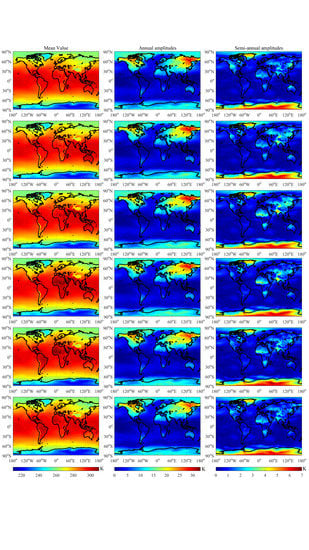
Figure 7 illustrates the mean values, annual amplitudes, and semi-annual amplitudes of temperature in Model #5; only the cases of UTC 0:00, 4:00, 8:00, 12:00, 16:00, and 20:00 are shown in the figure owing to the space limitation. The distribution of mean values is latitude-dependent and altitude-dependent; significantly small values appear at the poles and large values appear near the equator. The annual amplitudes become larger as the latitude increases, and the amplitudes at the land area are larger than those that at the ocean area. The maximum annual amplitude appears in the Siberian region because of its largest annual temperature difference. Affected by the phenomena of polar day and polar night, the Antarctic and Arctic regions exhibit large semi-annual amplitudes. Moreover, it is observed that changes of the mean values, annual amplitudes, and semi-annual amplitudes exist in different modelling epochs. This ensures that Model #5 can take good care of the diurnal variations. The model for pressure is similar to the case of temperature and will not be repeated in this paper.

The global distribution of RMS and MAE of the differences for pressure and temperature calculated by Model #5 is described in Figure 8, which shows the different performance of the model in various regions. For pressure, the accuracy decreased with the increasing of the latitude. For temperature, the low latitudes have better accuracy than the high latitudes and the ocean area performs better than the land area.

Moreover, the radiosonde data containing the surface’s temperature and pressure can be retrieved from the archive at the website of University of Wyoming (available on http://weather.uwyo.edu/ypperair/sounding.html). A total of 541 globally distributed radiosonde stations that contain available data over half a year of 2016 were selected. The surface temperature and pressure values of each station at UTC 0:00 and 12:00 every day in 2016 were regarded as the references to validate the accuracy of the meteorological parameters estimated by Model #5.

The statistical results of RMS for the two parameters are shown in Figure 9, in which the spatial variation in the accuracy of the model can be seen. It is observed that the accuracy of pressure and temperature calculated by Model #5 changes with the latitude. In low latitudes (<30º), the percentage of stations with pressure RMS less than 5 hPa is greater than 90% and the percentage reaches to 99% when focusing on the station with temperature RMS less than 5 K. An accuracy of better than 10 hPa for pressure RMS has been achieved at most stations worldwide; the percentage is 86% and the maximum RMS is 13.91 hPa. For the temperature RMS, most stations can achieve an accuracy of better than 6 K; the percentage reaches 89% and the maximum RMS is 8.4 K. In addition, the statistical results of the differences for temperature and pressure calculated by Model #5, including mean RMS, MAE, and SD, at the selected radiosonde stations are listed in

Table 4. Statistics of the differences for temperature and pressure calculated by Model #5 at the selected radiosonde stations.

	RMS	MAE	SD
Pressure (hPa)	7.02	5.24	6.46
Temperature (K)	4.05	3.17	3.86

, which shows that Model #5 can obtain pressure and temperature values that are consistent with the radiosonde data.

4. Discussion of the ZHD Accuracy Based on the Modelled Pressure and Temperature

In the GNSS sites without meteorological sensors equipped and co-located weather stations, the meteorological parameters estimated by above model can be used to calculate the ZHD. The most commonly used ZHD models, the Saastamoinen, Hopfield, and Black models, are selected in this paper to discuss the ZHD accuracy of different models based on the estimated pressure and temperature. In previous research, the three kinds of models were proved to achieve ZHD with high accuracy using measured meteorological data, and were widely used in GNSS meteorology [8,22,23,24,25,26,27,28]. The formulas are shown as follows [12,13,14,34,35]:

$$ZH{D}_S=0.002277\times P/\left(1-0.00266\cos 2\phi -0.00028h\right),$$

(6)

$$ZH{D}_H=1.522\times {10}^{-5}\times \left(40136+148.72\times \left(T-273.16\right)-h\right)\frac{P}{T},$$

(7)

$$ZH{D}_B=0.002343\left(T-4.12\right)\frac{P}{T},$$

(8)

where $ZH{D}_S$, $ZH{D}_H$, and $ZH{D}_B$ are the ZHD (unit: m) calculated by the Saastamoinen, Hopfield, and Black models, respectively. P and T refer to the estimated pressure and temperature, respectively. $\phi$ is the latitude and $h$ (unit: km) is the altitude. It can be seen that the Saastamoinen model only requires the pressure P (unit: hPa), but considers the effects of latitude and altitude. The temperature T (unit: K) and pressure P are included in the Hopfield and Black models, but the effect of latitude is not considered. The effect of altitude is considered in the Hopfield model, which is the difference between it and the Black model. Therefore, it is necessary to discuss the differences in calculating ZHD using various models based on estimated meteorological parameters on a global scale.

The website of global geodetic observing system (GGOS) Atmosphere (http://vmf.geo.tuwien.ac.at) can provide global atmospheric delay grid data including ZHD at a temporal resolution of 6 h, which is regarded as the true values of ZHD [36]. On the basis of the meteorological parameters estimated by Model #5, three kinds of computed ZHD values are obtained using the ZHD models mentioned above. The bias and RMS of the differences between the ZHD derived from the GGOS Atmosphere data and the ZHD calculated by the models at all grid points are counted and their global distribution is shown in Figure 10. Obviously, the distribution of bias and RMS of the Hopfield model is worse than the other two models, especially in the regions with high altitude, such as the Himalayas Mountains, the Andes Mountains, the Rocky Mountains, Greenland, and the Antarctic regions. This is mainly because the accuracy of the estimated temperature is relatively poor in these regions, and the accuracy of the Hopfield model is heavily dependent on temperature. It can be seen that the Saastamoinen and Black models can achieve good global accuracy in terms of RMS and bias. Their distributions of RMS and bias are latitude-dependent, where the larger and smaller values appear in higher and lower latitudes, respectively.

The statistical results of the different ZHD models are listed in

Table 5. Statistical results of different zenith hydrostatic delay (ZHD) models validated using global geodetic observing system (GGOS) Atmosphere data from 2016.

	Bias (mm)			RMS (mm)
	Max.	Min.	Mean	Max.	Min.	Mean
Saastamoinen model	61.1	−14.7	1.01	62.7	2.0	16.9
Hopfield model	78.5	−172.5	−13.0	172.6	2.5	30.7
Black model	62.4	−15.0	1.61	64.0	2.4	17.3

, in which the mean values of bias and RMS, as well as the maximum and minimum values, are shown. The Saastamoinen model with a mean bias of 1.01 mm and a mean RMS of 16.9 mm performs much better than the Hopfield model. The performance of the Black model with a mean bias of 1.61 mm and a mean RMS of 17.3 mm is slightly worse than that of the Saastamoinen model. The ranges of bias and RMS, that is, the maximum and minimum values, also prove the same conclusion.

In some grid points, the Hopfield and Black model can achieve better results than the Saastamoinen model. Therefore, the RMS differences at all grid points between the Saastamoinen and Hopfield model, as well as the Saastamoinen and Black model, are counted and their empirical distribution functions are plotted in Figure 11. Colors represent comparisons for different models in the figure, which indicates the percentage of each range of the RMS differences. It is observed that the percentage of grid points, of which the RMS of the Hopfield model is smaller than that of the Saastamoinen model, is more than 15%. For the case of the Black model, the percentage is more than 25%. The percentage of the RMS differences greater than 1 mm is 1.1% and 1.6% for the case of the the Hopfield and Black models, respectively. The largest RMS differences are 4.18 and 3.80 mm for the Hopfield and Black models, respectively. This illustrates that the specific analysis is needed in some regions to choose the appropriate ZHD model.

5. Conclusions

In this work, we analyzed the influence of different modelling factors on the global temperature and pressure model. Five kinds of model forms with different number of model coefficients were adopted to establish the models first, which indicated that there no obvious daily cycles existed in temperature lapse rate and specific humidity, and the daily cycle needs to be considered in the construction of the temperature and pressure model. The three kinds of model forms with consideration of daily cycles (Model #2, #3, and #4) implied that the adoption of sophisticated models (multiple model coefficients) did not necessarily improve the accuracy of the temperature and pressure. Model #5, with the idea of time-segmented modelling, performs best in this comparison. When the time resolution of the data sources is increased, from 6 h to 3 h and then to 2 h, only the accuracy of Model #5 is slightly improved. In this comparison, it is demonstrated that Model #5 can well describe the variation and fluctuation of temperature and the bimodality of pressure during a day. When the spatial resolution of the data source is increased, from 5° × 5° to 2.5° × 2°, the global mean RMS/MAE/SD of temperature and pressure are improved from 8.54/6.96/7.33 hPa and 3.38/2.67/3.15 K to 8.09/6.52/7.28 hPa and 3.25/2.55/3.10 K, from 8.36/6.78/7.28 hPa and 3.17/2.49/2.93 K to 7.94/6.39/7.25 hPa and 3.01/2.34/2.84 K, and from 8.29/6.73/7.21 hPa and 3.12/2.45/2.88 K to 7.87/6.33/7.17 hPa and 2.95/2.31/2.79 K, for Model #1, Model #3 and Model #5, respectively. To further show the accuracy of the Model #5 in the calculation of pressure and temperature, the comparison with radiosonde data was conducted and the mean RMS/MAE/SD are 7.02/5.24/6.46 hPa and 4.05/3.17/3.86 K for pressure and temperature, respectively. On the basis of the meteorological parameters estimated by Model #5, we analyzed the accuracy of the three most commonly used ZHD models without measured temperature and pressure. The numerical results showed that the Saastamoinen model with a global mean bias/RMS of 1.01/16.9 mm achieved the best performance. In the follow-up research, models with higher spatial resolution should be established to further improve the accuracy. For some certain grid points, the Saastamoinen model should be refined to better describe the ZHD values. Moreover, further research on how different the ZHD models would perform if the meteorological parameters were driven by different temperature and pressure models could be conducted.