An End-to-End Hyperspectral Scene Simulator with Alternate Adjacency Effect Models and Its Comparison with CameoSim

Abstract

In this research, we developed a new rendering-based end to end Hyperspectral scene simulator CHIMES (Cranfield Hyperspectral Image Modelling and Evaluation System), which generates nadir images of passively illuminated 3-D outdoor scenes in Visible, Near Infrared (NIR) and Short-Wave Infrared (SWIR) regions, ranging from 360 nm to 2520 nm. MODTRAN${}^{\mathrm{TM}}$ (MODerate resolution TRANsmission), is used to generate the sky-dome environment map which includes sun and sky radiance along with the polarisation effect of the sky due to Rayleigh scattering. Moreover, we perform path tracing and implement ray interaction with medium and volumetric backscattering at rendering time to model the adjacency effect. We propose two variants of adjacency models, the first one incorporates a single spectral albedo as the averaged background of the scene, this model is called the Background One-Spectra Adjacency Effect Model (BOAEM), which is a CameoSim like model created for performance comparison. The second model calculates background albedo from a pixel’s neighbourhood, whose size depends on the air volume between sensor and target, and differential air density up to sensor altitude. Average background reflectance of all neighbourhood pixel is computed at rendering time for estimating the total upwelled scattered radiance, by volumetric scattering. This model is termed the Texture-Spectra Incorporated Adjacency Effect Model (TIAEM). Moreover, for estimating the underlying atmospheric condition MODTRAN is run with varying aerosol optical thickness and its total ground reflected radiance (TGRR) is compared with TGRR of known in-scene material. The Goodness of fit is evaluated in each iteration, and MODTRAN’s output with the best fit is selected. We perform a tri-modal validation of simulators on a real hyperspectral scene by varying atmospheric condition, terrain surface models and proposed variants of adjacency models. We compared results of our model with Lockheed Martin’s well-established scene simulator CameoSim and acquired Ground Truth (GT) by Hyspex cameras. In clear-sky conditions, both models of CHIMES and CameoSim are in close agreement, however, in searched overcast conditions CHIMES BOAEM is shown to perform better than CameoSim in terms of ${\ell }_1$-norm error of the whole scene with respect to GT. TIAEM produces better radiance shape and covariance of background statistics with respect to Ground Truth (GT), which is key to good target detection performance. We also report that the results of CameoSim have a many-fold higher error for the same scene when the flat surface terrain is replaced with a Digital Elevation Model (DEM) based rugged one.

1. Introduction

Realistic assessment of detectability and vulnerability of targets is important in both civil and military applications. This requires the acquisition of high fidelity hyperspectral remote sensing images (HSI) for both targets and the background materials of the scene, which is time and cost-ineffective and, in some cases, it is even not possible to achieve through experimental trials. This drives the motivation of research to simulate remote sensing HSI data to allow the assessment of target detection capability under a variety of scene backgrounds, atmospheric conditions, sensor characteristics, ambient temperatures and light sources. Despite the existence of several commercial-off-the-shelf (COTS) HSI simulators within the remote sensing community, procurement, modification or enhancement of existing COTS simulation packages are prohibitive due to the export control and copyright protection issues. The objective of the present work is to establish a HSI simulator known as the Cranfield Hyperspectral Image Modelling and Evaluation System (CHIMES), which features an automatic atmospheric parameterization through a search algorithm to match the ground radiance of a given scene, and the proposal of two adjacency models to enhance the quality of the scene simulation. The output of the CHIMES is validated by a ground truth HSI scene and also compared with a COTS package CAMoflauge Electro-Optic Simulator (CameoSim).

The layout of the paper is as follows; Section 1 (this section) outlines the motivation and the objective of the present work; Section 2 gives an overview of the methodologies and capabilities of a few existing COTS scene simulator packages. Section 3 constitutes the main body of the paper which outlines the skeleton of the proposed CHIMES simulator with more details on the proposed adjacency models. Section 4 outlines the experimental data utilized in this work and Section 5 gives the analysis of the simulation outputs using a variety of statistical methods such as the band to band covariance statistics for eigenanalysis and also distance error measures. Section 6 summarizes the main achievements of the present work and the appendix gives detailed simulation results achieved by the proposed CHIMES and CameoSim.

2. Background Literature

2.1. Existing Simulators

Research interest in simulation of hyper-spectral imaging system has increased since the 1990s. The diversity of application areas for HSI scene modelling drives different motivations behind the development of such models and software applications. A detailed list of existing simulators, their motivation and capacity is covered in subsequent sections with a brief overview in

Table 1. Hyperspectral scene simulators, their developers, year of development, primary objective, spectral bands and model types. DISORT algorithm [1] is an integral part of MODTRAN which is used to calculate scattering and adjacency effect.

Simulators	Developed By	Primary Objective	Spectral Bands ($\mathsf{\mu }$m)	Model Type	Adjacency-Effect Modelling	Noise Modelling
FASSP (1996–)	MIT Lincoln’s Lab	Sensor Modelling	0.3–2.5	MODTRAN-based Statistical Estimation	DISORT	Yes
CameoSim (1998–)	Lockheed Martin/Insys	Camoflauge Assessment	0.3–20.0	Light Transport (Radiosity)	DISORT	No
DIRSIG 1–4 (1997–2015)	RIT	HS Image Generation	0.3–20.0	Light Transport (Whitted Ray-tracing)	DISORT	Yes
DIRSIG 5 (2015–)	RIT	HS Image Generation	0.3–20.0	Light Transport (Metropolis Light Transport)	DISORT/MODTRAN6	Yes
OSSIM (2004–)	Denel SOC Ltd	Countermeasure	0.4–20.0	Light Transport (Safir-based Ray-tracing)	DISORT	Yes
MCScene (1999–)	Spectral Science	HS Image Generation	0.3–20.0	Direct Simulation Monte-Carlo	DISORT	Yes
ATCOR (2006–)	ReSe	Atmospheric Compensation	0.3–14.0	MODTRAN-based Radiance Estimation	Own Model	Yes
PICASSO (1999–)	MIT Lincoln’s Lab	Sensor Modelling	0.3–14.0	MODTRAN-based Radiance Estimation	DISORT	Yes
EnMap (2009–)	DLR	Sensor Modelling	0.3–2.5	MODTRAN-based Radiance Estimation	DISORT	N/A
CHIMES (2017–)	Cranfield University	HS Image Generation	0.3–2.5	Light Transport (Path-tracing)	DISORT	No

.

2.1.1. Forecasting and Analysis of Spectroradiometric System Performance (FASSP)

FASSP is one of the earliest attempts in this area, which pursued a statistical parametric modelling approach. FASSP is a statistical model for the analysis of earth observing data acquired by optical spectral imaging systems. The predominant surface parameters considered are the spectral reflectance mean vector and spectral covariance matrix [2].

FASSP architecture provide identification of the primary components of the scene for the simulation [3], these components are one of the building blocks for our proposed simulator, however, we extended their components to include rendering and image reconstruction as supplementary ones. Our revised components of a scene simulator and data flow is shown in Figure 1.

2.1.2. Digital Imaging and Remote Sensing Image Generation (DIRSIG)

DIRSIG adopts an image-chain approach to Remote-Sensing simulation. It is capable to simulate passive broadband, multi-spectral, hyper-spectral, low-light, polarized, active laser radar, and synthetic aperture radar datasets. Its components include bi-directional reflectance distribution function (BRDF) predictions of a surface, time and material dependent surface temperature predictions, to the dynamic viewing geometry of scanning imaging instruments on agile ground, airborne and space-based platforms [4,5,6,7]. In a recent update called DIRSIG5 [8] Metropolis Light Transport (MLT) based path tracing has been used. Atmospheric processing can be performed by both MODTRAN5 and MODTRAN6 [9].

2.1.3. CAMoflauge Electro-Optic Simulator (CameoSim)

CameoSim is a commercial scene simulator originally developed for the assessment of camouflage systems, from the far Infra-Red, visible and to the UV with HSI capabilities [10]. It uses raytracing with a Monte-Carlo radiosity light-transport scheme. All the geometric objects forming the synthetic environment are modelled using textured faceted structures. Texel values in these textures are mapped to the real materials associated with them [11,12]. These materials can have measured properties using one of several BRDF models, with optional transparency. It supports moving observers and players, with moving parts. It can handle large complex scenes with billions of pixels and is applicable to ground, ocean, air and space scenarios. It can model plumes and flares. It predicts surface temperatures, with optional thermal shadowing, using weather measurements. Atmospherics can be generated using MODTRAN 5, or measured atmospherics imported. Environmental maps based on High Dynamic Range (HDR) images can be imported for scene simulation.

2.1.4. Optronic Scene Simulator (OSSIM)

OSSIM is another HSI scene simulator that creates synthetic images of arbitrary complex scenes by rendering, the spectral range is in the visual and infrared (IR) bands, covering the 0.4–20 $\mathsf{\mu }$m spectral region. These images are radiometrically accurate and based on theoretical physics models. To allow for the subtleties and full scope of variability in atmospheric attenuation, the simulation employs all capabilities of the MODTRAN. The geometrical shape of objects and the terrain topography is described in terms of a three-dimensional complex hull, consisting of a set of flat, convex facets or polygons. Each polygon is assigned spectral radiometric properties, temporally variable spatial texture properties and radiometric properties. Polygons can also be partially transparent to represent gas clouds, countermeasure flares or aircraft plumes [13,14,15,16].

2.1.5. Monte-Carlo Scene (MCScene)

MCScene is also a rendering-based HSI scene simulator. It incorporates all optical effects important for solar-illuminated and thermal scenes, including molecular and aerosol scattering, absorption and emission and surface scattering with material-dependent bidirectional reflectance distribution functions (BRDFs), multiple scattering events, surface adjacency effects, and scattering, emission and shading by clouds, for arbitrary solar illumination and sensor viewing geometries. The “world” of the simulation is a cube that encloses a user-definable atmosphere containing molecular species, aerosols, and clouds, and a terrain representing the ground. The sensor spatial and spectral resolution, its location, and the viewing angle are also specified. 3D objects can also be inserted into the scene. A particular strength of MCScene is that a simulation can be data-driven. Terrain information can be imported from United States Geological Surveys (USGS) digital elevation maps. Surface reflectance or emissivity/temperature maps can be derived from collected imagery, thus incorporating natural spectral and spatial texturing into a simulation [17,18,19,20].

2.1.6. Parameterized Image Chain Analysis & Simulation SOftware (PICASSO)

PICASSO is also one of the end-to-end HSI image simulation or image chain analysis tools which estimate at-sensor radiance based on MODTRAN. Simulation flow begins with a description of the remote sensing system to be modelled, in terms of standard engineering parameters (e.g., primary aperture diameter, effective focal length, focal plane array detector size, focal plane array operating temperature, etc.). PICASSO also requires an input earth scene that can serve as ground-truth. The principal output of PICASSO is a simulated image, having the characteristics that would be produced by the remote sensing system under simulation. In addition to this simulated image, PICASSO produces figures of merit commonly used throughout the remote sensing industry to characterize image quality. These can include such metrics as SNR for given radiance; plots of the system transfer function (STF) and point-spread function (PSF) or overall image quality as measured by the National Imagery Interpretability Rating Scale (NIIRS) [21,22].

2.1.7. The Environmental Mapping and Analysis Program (EnMAP)

ENMAP is a German hyperspectral satellite mission that aims at monitoring and characterising the Earth’s environment on a global scale. The hyperspectral imager is a push-broom type consisting of two prism imaging spectrometers—one for VNIR (Hyspex VNIR1600) and one for SWIR (Hyspex SWIR320m). As a precursor of the mission, EnMAP simulator was developed. The EnMAP scene simulator is able to generate realistic EnMAP-like data in an automatic way under a set of user-driven instrument and scene parameters. Radiance and digital numbers data are generated by five sequential processing modules which are able to produce data over a range of natural environments, acquisition and illumination geometries, cloud covers, and instrument configurations. The latter include the simulation of data nonuniformity in the spatial and spectral domains, spatially coherent and noncoherent instrumental noise, and instrument’s modulation transfer function (MTF). Realistic surface patterns for the simulated data are provided by existing remote-sensing data in different environments, from dry geological sites to green vegetation areas. A flexible radiative transfer simulation scheme enables the generation of different illumination, observation, and atmospheric conditions [23].

2.2. Light Transport based Simulators and Radiative Transfer Models

In this section, the radiative transfer (RT) equations of light-transport based models are discussed. The general RT equation for at-sensor radiance within an optical spectrum is given as Equation (1), [24]. Rendering based simulators perform integration by Monte-Carlo method, while approximate methods assume Lambertian BRDF. DIRSIG’s big equation, which is given in Equation (2), also assumes Lambertian BRDF to yield an analytical form of Equation (1). We also adopt Equation (2) for convention and to elaborate alternate treatments of upwelled scattered term only, which is our focus.

$$\begin{array}{c}Ls({\theta }_i,{\theta }_r,\varphi ,\rho ,{\Omega }_i)=\hfill \\ \hfill f_r({\theta }_i,{\theta }_r,\varphi )E_s\left({\theta }_i\right)cos\left({\theta }_i\right){\tau }_i\left({\theta }_i\right){\tau }_r\left({\theta }_r\right)\rho +{\tau }_r\left({\theta }_r\right)\rho {\int }_F{\int \int }_{\Omega i}{f}_r({\theta }_i,{\theta }_r,\varphi )cos\left({\theta }_i\right)L_d^{{\Omega }_i}({\theta }_i,\varphi )d{\Omega }_i+L_p({\theta }_i,\varphi ),\end{array}$$

(1)

where $Ls$ is total at-sensor radiance, $f_r$ is the Bidirectional Reflection Distribution Function (BRDF) [25], $E_s$ is exoatmospheric solar spectral irradiance, ${\tau }_i$ and ${\tau }_r$ are incident and reflected transmittance, $L_p$ is path radiance, F is the view factor of sky, and solid angle ${\Omega }_i$ is given as d${\Omega }_i$ = sin${\theta }_i$d${\theta }_i$d$\varphi$. ${\theta }_i$, and ${\varphi }_i$ are solar zenith and azimuth angles, respectively, ${\theta }_r$ is a reflected ray angle with respect to surface normal and $\rho$ is target reflectance.

RT equations implemented in various versions of simulators, such as the DIRSIG, CameoSim, and ATCOR are slightly different. This is mainly because of the various adjacency models that have been employed by these simulators are slightly different. For example, version 4 of the DIRSIG employs the Whitted-style ray tracing, while CameoSim renders by radiosity and the proposed CHIMES adopts the path-tracing strategy for computing the at-sensor radiance. Thus the performance of the HSI simulator is greatly affected not only by the atmospheric or environmental factors, but also the blend of computer graphics parameters such as the ray sampling strategy, the reconstruction filtering knowledge and also the graphical rendering techniques which all impose impacts to the quality of the simulation.

In ray tracing, there are three types of rays—reflected, refracted, and shadow when a ray interacts with an obscured surface. A ray continues its specular reflected direction when it hits a shiny surface. Refracted rays travel through transparent material may be entering or exiting a material. Although it is a recursive process, however, to avoid tracing all rays in a scene, a shadow ray is used to test if a surface is visible to the light. If this test is true then a ray is traced between this intersection point and the light. In the case of path tracing, a path history of a single point is created when a ray interacts with the environment until it is fully absorbed. That is, rather than to spawn new rays at the intersection point, it simply chooses a direction as according to the BRDF of the surface and to assign the direction for the ray to follow. A number of random rays per pixel are then sampled using the Monte-Carlo method and the final at-sensor radiance is computed through image reconstruction filter, which rasterizes the accumulated radiance. An important property of path tracing is that the computation is more emphasis on those low-depth rays, while the Whitted ray tracing concerns more of the high-depth rays. The rendering in CameoSim uses radiosity method which will be described in more detail in Section 2.2.2.

2.2.1. DIRSIG

DIRSIG utilizes the RT Equation called Big Equation [4,7], having radiance components of different types of rays as illustrated in Figure 2. Assuming the BRDF of the target object conforms to Lambertian which reduces the big equation into the analytical form as shown in Equation (2). According to reference [26] the "I" type ray can be grouped together with the "C" type if the average albedo of the scene is slowly varying, which is common [15] in relatively homogeneous scenes. DIRSIG employs an image-chain differential thermodynamic model to evaluate the temperature of background objects in the scene. It accounts for both optical and thermal shadows caused by full or partial occlusion due to the opaqueness of the transmissive objects. The loss due to the interaction of rays between the media and the transmittance of objects can also be accounted for during rendering.

$$\begin{array}{c}L\left(\lambda \right)={\tau }_2\left(\lambda \right)\{\stackrel{A}{\overbrace{\underset{\mathrm{reflected}\mathrm{sunshine}}{\underbrace{\frac{E_s^{\prime }\left(\lambda \right)}{\pi }{\tau }_1\left(\lambda \right)\rho \left(\lambda \right)cos\sigma }}}}+\stackrel{D}{\overbrace{\underset{\mathrm{thermally}\mathrm{emitted}}{\underbrace{ϵ\left(\lambda \right)L_T\left(\lambda \right)}}}}+\underset{\mathrm{reflected}\mathrm{sky}}{\underbrace{{\rho }_d\left(\lambda \right)F\left[\stackrel{B}{\overbrace{\frac{E_{ds}\left(\lambda \right)}{\pi }}}+\stackrel{E}{\overbrace{\frac{E_{dϵ}\left(\lambda \right)}{\pi }}}\right]}}+\hfill \\ \hfill \underset{\mathrm{reflected}\mathrm{background}}{\underbrace{{\rho }_d\left(\lambda \right)(1-F)\left[\stackrel{G}{\overbrace{L_{bs}\left(\lambda \right)}}+\stackrel{H}{\overbrace{L_{bϵ}\left(\lambda \right)}}\right]}}\}+\underset{\mathrm{atmospheric}\mathrm{path}\mathrm{radiance}}{\underbrace{\stackrel{C+I}{\overbrace{L_{us}\left(\lambda \right)}}+\stackrel{F}{\overbrace{L_{uϵ}\left(\lambda \right)}}}}.\end{array}$$

(2)

DIRSIG uses MODTRAN for its atmospheric processing. It also creates a sky-dome environment map for illumination which is created by MODTRAN based lookup tables [27]. The texture applied to geometry is used as material and thermodynamic database identifier [13]. Symbols of Equation (2) are explained in

Table 2. Symbols in Equation (2) and their meaning, $\lambda$ shows that quantities are function of wavelength.

Symbol	Meaning	Symbol	Meaning
$E_s^{\prime }$($\lambda$)	Exoatmospheric irradiance	1-F	Fraction of hemisphere above target that is background
$\sigma$	Solar zenith angle w.r.t target normal	$E_{ds}$($\lambda$)	Downwelled solar irradiance
${\tau }_1$($\lambda$)	Transmittance along sun-target path	$E_{dϵ}$($\lambda$)	Downwelled self-emitted radiance from the atmosphere
${\tau }_2$($\lambda$)	Transmittance along target-sensor path	${\rho }_d$($\lambda$)	Target diffuse reflectance
$\rho$($\lambda$)	Target reflectance	$L_{bs}$($\lambda$)	Background reflected solar radiance onto target
$ϵ$($\lambda$)	Target emissivity	$L_{bϵ}$($\lambda$)	Background self emitted irradiance onto target
$L_T$($\lambda$)	Self emitted radiance from target at temperature T	$L_{us}$($\lambda$)	Upwelled solar irradiance
F	Fraction of hemisphere above target that is sky	$L_{uϵ}$($\lambda$)	Upwelled self-emitted radiance
$\rho \left(\lambda \right)$	Target direct reflectance

.

2.2.2. CameoSim

CameoSim is one of the earliest commercial HSI simulators and is feature-rich. It can require some effort from the end-user if all its features are to be exploited. CameoSim is developed in a modular fashion therefore features are divided into modules’ user interfaces, typically called editors. Figure 3 shows components of CameoSim and data flow.

In the process of generating radiometrically accurate synthetic images of scenes, all sources in the synthetic environment affect the solution of a rendering equation. The rendering equation for a general radiosity model is given in Equations (3)–(6). The three main components of the rendering equation are the thermal self-emission, the atmospheric terms, global illumination accounting for reflected radiance. In CameoSim, a general bidirectional, spectral, recursive solution is sought using importance driven Monte-Carlo sampling. At longer wavelengths, such as mid-infrared, the full hemispherical integration of incident irradiances enable the software to account for the radiative interaction between different surfaces at varying thermodynamical states. BRDF models take account of bi-directional light reflecting properties of a surface, in CameoSim it is termed as (surface) scatter models, as shown in Figure 3.

Figure 4 illustrates components of a radiosity rendering equation. Bidirection Reflection Distribution Function (BRDF) and Bidirectional Transmission Distribution Funtion (BTDF) represent the surface response on interaction with rays. Geometrical definition of sources is shown in Figure 4b and the hemispherical integration is included in Figure 4c. Equations (3)–(6) shows the rendering equation for CameoSim. Symbols and their meaning are explained in

Table 3. Symbols in Equations (3)–(6) and their meaning.

Symbol	Meaning	Symbol	Meaning
${\omega }_o$	Observer or sensor direction or position	$L_i$(x, ${\omega }_t$)	Radiance incident on x from direction ${\omega }_t$
x	A point on the target surface	$L_t$(x, ${\omega }_t$)	Radiance transmitted through point x in the direction of ${\omega }_t$.
${\omega }_t$	Incident direction of transmitted radiance w.r.t x	$f_t$(${\omega }_o$, x, ${\omega }_t$)	Bidirectional reflectivity at point x with respect to directions ${\omega }_o$ and ${\omega }_i$
${\omega }_i$	Incident direction of emitter’s radiance w.r.t. x	$f_t$(${\omega }_o$, x, ${\omega }_t$)	Bidirectional transmittivity at point x with respect to directions ${\omega }_o$ and ${\omega }_i$
$L_{path}$(${\omega }_o$, x)	Radiance along target-sensor path
$L_e$(x,${\omega }_o$)	Radiance emitted from point x, towards direction ${\omega }_o$
$L_r$(x,${\omega }_o$)	Radiance reflected from x in the direction of ${\omega }_o$
$L_i$(x, ${\omega }_i$)	Radiance incident on x from direction ${\omega }_i$

.

$$L_o(x,{\omega }_o)=L_{path}(x_1,x_2)+L_e(x,{\omega }_o)+L_r(x,{\omega }_o)+L_t(x,{\omega }_t)$$

(3)

$$L_r(x,{\omega }_o)={\int }_{\Omega }{f}_r(x,{\omega }_i\to {\omega }_o)L_i(x,{\omega }_i)cos{\theta }_{i}d{\omega }_i$$

(4)

$$L_t(x,{\omega }_o)={\int }_{\Omega }{f}_t(x,{\omega }_t\to {\omega }_o)L_i(x,{\omega }_t)cos{\theta }_{t}d{\omega }_t$$

(5)

$$\begin{array}{c}{L}_o(x,{\omega }_o)=L_{path}(x_1,x_2)+L_e(x,{\omega }_o)+{\int }_{\Omega }{f}_r(x,{\omega }_i\to {\omega }_o)L_i(x,{\omega }_i)cos{\theta }_{i}d{\omega }_i+\hfill \\ \hfill {\int }_{\Omega }{f}_t(x,{\omega }_t\to {\omega }_o)L_i(x,{\omega }_t)cos{\theta }_{t}d{\omega }_t.\end{array}$$

(6)

2.3. Adjacency Effect Models

2.3.1. MODTRAN

MODTRAN adopts the DISORT algorithm with a variable number of streams for scattering and adjacency modelling. At-sensor apparent reflectance ${\rho }_a$ is given in Equation (7).

$${\rho }_a=\frac{\pi L_s}{E_s^{\prime }cos\theta }.$$

(7)

The upward surface flux that is reflected by the atmosphere back to the ground and then reflected by the ground ${\overline{\rho }}_b$ upwards. Since this phenomena occur multiple times before it is finally scattered into the LoS of the sensor, therefore it takes the form of power series as given in Equation (8).

$$({\tau }_1^{\mathit{dir}}+{\tau }_1^{\mathit{dif}})({\tau }_2^{dir}{\rho }_t+{\tau }_2^{\mathit{dif}}{\overline{\rho }}_b)\left[1+s{\overline{\rho }}_b+{\left(s{\overline{\rho }}_b\right)}^2+\dots \right]=\frac{({\tau }_1^{\mathit{dir}}+{\tau }_1^{\mathit{dif}}){\tau }_2^{dir}{\rho }_t}{1-s{\overline{\rho }}_b}+\frac{({\tau }_1^{\mathit{dir}}+{\tau }_1^{\mathit{dif}}){\tau }_2^{\mathit{dif}}{\overline{\rho }}_b}{1-s{\overline{\rho }}_b}.$$

(8)

At-sensor apparant reflectance ${\rho }_a$ can be redefined in terms of Equation (8) as Equation (9) [28].

$${\rho }_a={\rho }_o+\frac{({\tau }_1^{\mathit{dir}}+{\tau }_1^{\mathit{dif}}){\tau }_2^{dir}{\rho }_t}{1-s{\overline{\rho }}_b}+\frac{({\tau }_1^{\mathit{dir}}+{\tau }_1^{\mathit{dif}}){\tau }_2^{\mathit{dif}}{\overline{\rho }}_b}{1-s{\overline{\rho }}_b},$$

(9)

where ${\rho }_o$ is the path reflectance. In order to calculate the total upwelled scattered reflectance term, ${\rho }_t$ should be set to zero, which is target albedo during MODTRAN run. Therefore Equation (9) takes the form of Equation (10).

$${\rho }_u={\rho }_o+\frac{({\tau }_1^{\mathit{dir}}+{\tau }_1^{\mathit{dif}}){\tau }_2^{\mathit{dif}}{\overline{\rho }}_b}{1-s{\overline{\rho }}_b},$$

(10)

where ${\rho }_u$ is the upwelled scattered apparant reflectance. It includes both path reflectance and adjacent reflectance, in the first and the second term, respectively.

Symbols used in Equations (7)–(10) are explained in

Table 4. Symbols in Equations (8) and (9) and their meaning.

Symbol	Meaning	Symbol	Meaning
${\rho }_o$	Path reflectance	${\tau }_2^{\mathit{dif}}$	Ground to sensor diffuse transmittance
${\tau }_1^{dir}$	Sun to ground direct transmittance	s	spherical scattering albedo of the atmosphere
${\tau }_1^{\mathit{dif}}$	Sun to ground diffuse transmittance	${\rho }_t$	Target reflectance
${\tau }_2^{dir}$	Ground to sensor direct transmittance	${\overline{\rho }}_b$	Area averaged background reflectance

.

2.3.2. CameoSim

Although CameoSim provides surface scattering through built-in BRDF models, it does not include volumetric scattering during the texture rendering. CameoSim treats the adjacency through the DISORT models of the upwelled scattered radiance, which means the adjacency is dependent only on a single source of spectral albedo, that is, the average background albedo of the scene.

2.3.3. DIRSIGs

DIRSIG5 handles adjacency effect by considering all rays that are scattered into the sensor from outside of its Field Of View (FOV) through the path tracing. This volumetric scattering is driven by the atmospheric phase function of the scene [29], but in this version of the simulator, the scattering efficiency as a function of the sensor altitude has not been taken into account. Older version of DIRSIG, that is, DIRSIG4 incorporated atmospheric variability [27] and adjacent scattered light can be grouped with the path radiance particularly when the averaged background albedo of the scene is slowly varying [26]. Hence the adjacency in DIRSIG4 is functioning like that of the CameoSim, which utilizes a single stream of the background albedo for the DISORT calculation.

2.3.4. ATCOR

Although ATCOR is not an HSI scene simulator, it features an adjacency model which does not employ rendering for the estimation of the observed at-sensor radiance in its atmospheric correction package [30]. Jianwen et al. [31] conducted a series of measurement to estimate adjacency effect, they reported that the adjacency effect becomes stronger from visible, near-infrared to shortwave infrared wavelength. In response to this work, Reference [32] presented Equation (14) to include the effect of contrast between the target and background pixels in at-sensor radiance. Before deriving ATCOR’s model the RT equation can be rephrased in terms of atmospheric spherical albedo for a “large surface” with reflectance $\rho$, as follows [33,34],

$$L_s\left(\rho \right)=L_p+\frac{\tau E_g\left(0\right)\rho /\pi }{1-s\rho },$$

(11)

where $\tau$, $E_g\left(0\right)$, and s are the total ground-to-sensor transmittance, global flux on the ground for $\rho$ = 0, and the spherical albedo of the atmosphere, respectively. $\tau$ is the sum of the direct and diffuse transmittance, that is, $\tau$ = ${\tau }_{\mathrm{dir}}$ + ${\tau }_{\mathrm{diff}}$. Equation (11) shows that the effective global flux is;

$$E_g\left(\rho \right)=\frac{E_g\left(0\right)}{1-\mathrm{s}\rho }$$

(12)

and it depends on the ground reflectance and spherical albedo [32]. However, for “small target” of reflectance ${\rho }_t$, the at-sensor radiance is calculated as given in reference [34].

$$Ls\left(\rho \right)=L_p+\frac{{\tau }_{dir}{E}_g\left(0\right){\rho }_t/\pi }{1-s{\overline{\rho }}_b}+\frac{{\tau }_{dif}{E}_g\left(0\right){\overline{\rho }}_b/\pi }{1-s{\overline{\rho }}_b}.$$

(13)

Furthermore, Richter et al. [32] rewrote Equation (13) to accommodate the contrast term;

$$Ls\left(\rho \right)=L_p+\frac{\tau E_g\left(0\right){\rho }_t/\pi }{1-s{\overline{\rho }}_b}+\frac{{\tau }_{dif}{E}_g\left(0\right)({\overline{\rho }}_b-{\rho }_t)/\pi }{1-s{\overline{\rho }}_b}.$$

(14)

Equation (14) emphasizes the fact that the adjacency term is directly proportional to the target background reflectance contrast. ATCOR also includes sensor height based scattering efficiency calculation based on air density, and volume between the sensor and the target material.

3. Proposed CHIMES Simulator

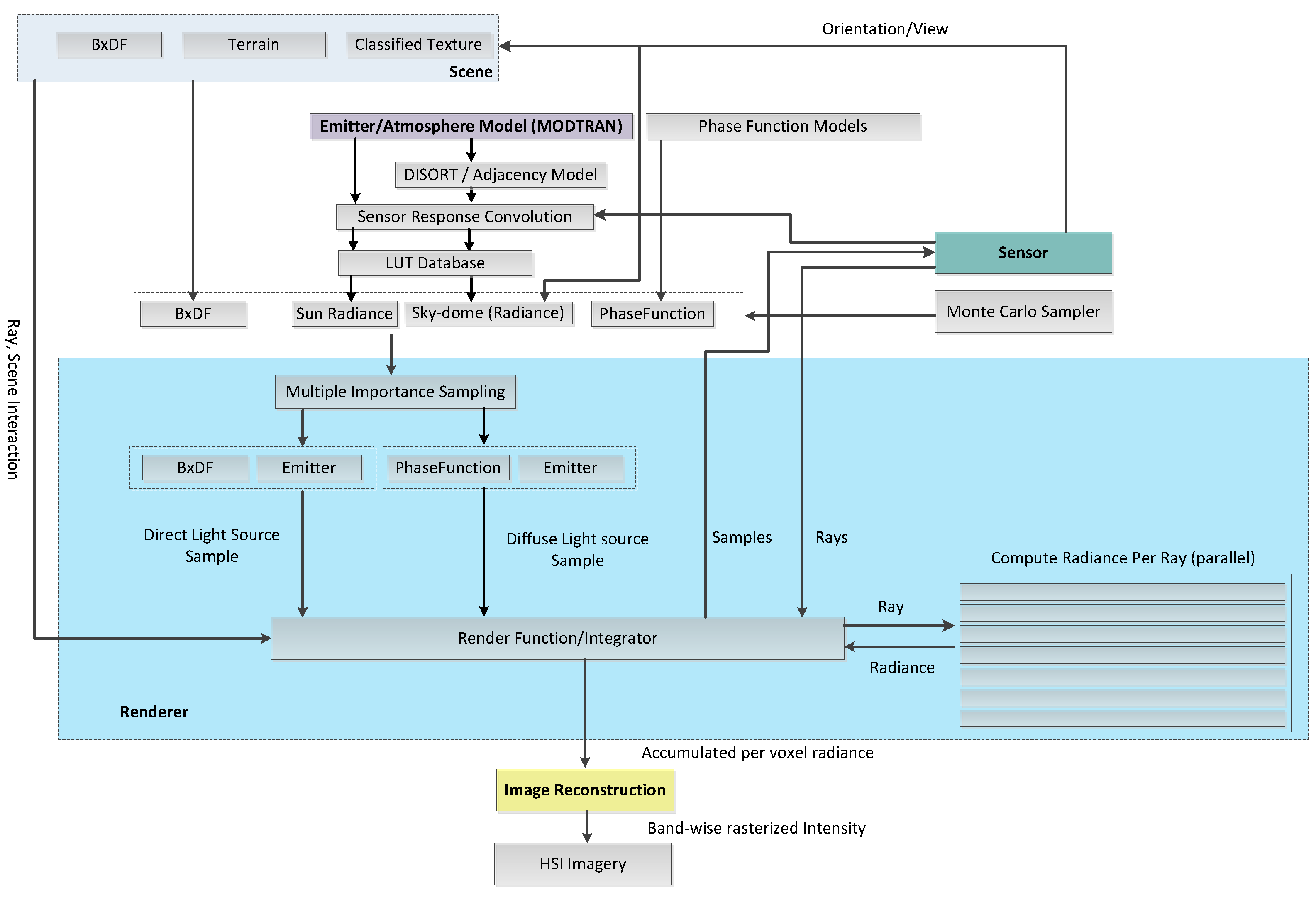
CHIMES is a texture rendering based simulator and an overview of its design and system components are shown in Figure 1 and Figure 5 respectively. As mentioned in the introduction section, there are two main features in the proposed CHIMES; one is enhanced adjacency treatment that has been implemented for a better estimation of the volumetric scattering of upwelled scattered radiance, which is particularly important for the simulation of rugged scenes. This feature is in the form of a regional background neighbourhood function, which, embeds an altitude dependence of the optical scattering characteristics between the ground and the sensor. During the simulation, the averaged background albedo of the surrounding region of the test pixel, and the total upwelled radiance are evaluated for each pixel in the scene during the rendering process. The use of this neighbourhood function together with volumetric scattering has not been found in the open domain, and it is believed that this approach may help to enhance the performance of other scene simulators in the community. DIRSIG5 offers volumetric scattering based adjacency model, however considering effective background neighbourhood based on sensor height, air volume and density is not reported. Although ATCOR also employs the neighbourhood based adjacency, however, it performs differencing of target and background spectra to model the reduced contrast. This is only an approximation because volumetric scattering is not considered in ATCOR, probably due to its application domain. Moreover, variable height difference from every pixel to the sensor is not also considered in ATCOR or any other COTS scene simulation package.

The other feature in the CHIMES is the automatic search of the optimal atmospheric parameters to be used for the simulation of a scene, such that the output will be as realistic as that of the ground truth data. Many simulators, such as the DIRSIG and the CameoSim, require the user to define the atmospheric parameters which are unknown. Thus a number of trial and error of simulation runs using different sets of atmospheric parameters are normally required for these simulators. This contribution will help to reduce the amount of guesswork and help to obtain the optimal simulation result without repeatedly trial and error processing by varying the aerosol optical thickness.

3.1. Proposed Adjacency Models for CHIMES Simulator

The adjacency effect reduces with wavelength [32] as it depends on scattering efficiency. In CHIMES we maintain most of DIRSIG radiative transfer equation, however, treatment of I type of rays (adjacency) is handled with two different models. Both of our models adopt DISORT based upwelled scattering, however approach of setting average background albedo ${\overline{\rho }}_b$ is different in them. Our first and comparably simplistic model is similar to CameoSim.

Based on Equation (10), the upwelled scattered radiance into the sensor is therefore expressed as in Equation (15). This is the path radiance output from MODTRAN when target albedo is set to zero, during execution.

$$L_{us}^m=\frac{{\rho }_u{E}_s^{\prime }cos\theta }{\pi }.$$

(15)

Replacing upwelled scattered term of Equation (2) by Equation (15) we get Equation (16), which is the lambertian BRDF form of CHIMES Background One-Spectra AEM (BOAEM) model. The final estimation of $L_{us}^m$ during rendering is driven by volumetric scattering. This model is constructed to provide a better comparison of CHIMES with CameoSim, in terms of overall performance, which include several parameters such as sensor model, scene, ray tracing, volumetric scattering and background reflected radiance and so forth.

$$L\left(\lambda \right)={\tau }_2\left(\lambda \right)\left\{\frac{E_s^{\prime }\left(\lambda \right)}{\pi }{\tau }_1\left(\lambda \right)\rho \left(\lambda \right)cos\sigma +ϵ\left(\lambda \right)L_T\left(\lambda \right)+{\rho }_d\left(\lambda \right)F\left[\frac{E_{ds}\left(\lambda \right)}{\pi }+\frac{E_{dϵ}\left(\lambda \right)}{\pi }\right]+{\rho }_d\left(\lambda \right)(1-F)\left[L_{bs}\left(\lambda \right)+L_{bϵ}\left(\lambda \right)\right]\right\}+\frac{{\rho }_u{E}_s^{\prime }cos\theta }{\pi }+L_{uϵ}\left(\lambda \right).$$

(16)

In the second, more comprehensive, adjacency model, CHIMES adopts the methodology similar to that in ATCOR to deduce the upwelling of the adjacency through a sliding window of regions along the horizontal scale of the terrain. Since the extent of the adjacency scattering depends on the density of air within the field of view of the sensor, hence the adjacency is a function of the sensor altitude ($h_1$) and the elevation of ground ($h_2$). Through experimental analysis Richter et al. [35] derived an empirical equation to quantify the approximate adjacency range $R(h1,h2)$ on the ground as;

$$R=(h_1-h_2)0.1.$$

(17)

The above empirical equation is the result of the air density differentiation along elevation z. It has been shown that the density of air $D\left(z\right)$ is exponentially reduced above $z_d$ elevation;

$$D\left(z\right)=D_{o}exp\left(\frac{-z}{z_d}\right),$$

(18)

where $D\left(z\right)$ is air density at altitude z, $D_o$ represents density at sea-level and $z_d$ is the average scale height for the density of air which is 8 Km [35]. The adjacency effect for every pixel in a scene is evaluated by forming a region of interest (ROI) of $(2R\times 2R)$ pixels having the test pixel (target) in the center. According to Equation (17) the dimension of the ROI is dependent on the difference of elevation of the test pixel (target) and sensor altitude. Therefore in rugged terrain’s ROI dimension is variable across the scene. For each pixel in the scene, CHIMES deduces the path reflectance (${\rho }_o$), adjacent contribution for unit reflectance ($\Delta {\rho }_u$) and the ROI background reflectance ( ${\overline{\rho }}_{bK}$ ) for each $(2R\times 2R)$ ROI. We incorporate ${\overline{\rho }}_{bK}$ into Equation (2) by interpolation, therefore ${\rho }_u$ is calculated for ${\overline{\rho }}_b=0.0$ and ${\overline{\rho }}_b=1.0$ from Equation (10), and it is denoted by ${\rho }_{u0}$ and ${\rho }_{u1}$, respectively which is given in Equation (19). Interpolation between zero and one is performed in these experiments due to large test scene and memory constraints which may incur interpolation errors, therefore it is recommended to calculate ${\rho }_u$ from MODTRAN at more intermediate points between zero and one.

$$\begin{array}{c}\hfill {\rho }_{u0}={\rho }_o\end{array}$$

(19a)

$$\begin{array}{c}\hfill {\rho }_{u1}={\rho }_o+\frac{({\tau }_1^{\mathit{dir}}+{\tau }_1^{\mathit{dif}}){\tau }_2^{dir}}{1-s}\end{array}$$

(19b)

$$\begin{array}{c}\hfill \Delta {\rho }_u={\rho }_{u1}-{\rho }_{u0}=\frac{({\tau }_1^{\mathit{dir}}+{\tau }_1^{\mathit{dif}}){\tau }_2^{dir}}{1-s}.\end{array}$$

(19c)

${\overline{\rho }}_{bK}$, inside ROI is calculated by Equation (20).

$${\overline{\rho }}_{bK}=\sum _{s=1}^M\frac{{\rho }_s}{R_s^2},$$

(20)

where ${\rho }_s$ is the reflectance of the sample pixel as shown by red pixels depicted in Figure 6b and $R_s$ is the distance between target pixel (green/orange) and sample pixels. M is the number of samples in the grid. The upwelled scattered reflectance for the ROI region is therefore computed according to every pixel’s position and height by interpolation as given in Equation (21), where Subscript K denotes the kernel ROI. The approximate upwelled scattered radiance for the ROI is given in Equation (22).

$$\begin{array}{c}\hfill {\rho }_{uK}={\rho }_{u0}(1-{\overline{\rho }}_{bK})+{\overline{\rho }}_{bK}{\rho }_{u1}\end{array}$$

(21a)

$$\begin{array}{c}\hfill {\rho }_{uK}={\overline{\rho }}_{bK}\Delta {\rho }_u+{\rho }_{u0}\end{array}$$

(21b)

$$L_{usK}^m=\frac{({\overline{\rho }}_{bK}\Delta {\rho }_u+{\rho }_{u0})E_s^{\prime }cos\theta }{\pi }.$$

(22)

Once ${\overline{\rho }}_{bK}$ is computed for the intersecting ray, it is backscattered by coupling the phase function of the atmosphere and the diffuse emitter in ray-tracing by utilizing Monte- Carlo multiple importance sampling [36]. A ray-level computation of upwelled scattered radiance is shown in Figure 6a. Moreover, the actual model in CHIMES also considers BxDF models in calculating the radiance. It should be noted that, unlike ATCOR, TIAEM does not perform any differencing between target and background reflectance. Contrast reduction is the consequence of volumetric backscattering of the computed upwelled scattered radiance under the kernel, which eventually takes the form of Equation (22). The final rendering equation for the TIAEM model (assuming Lambertian BRDF) takes the form of Equation 23.

$$\begin{array}{c}L\left(\lambda \right)={\tau }_2\left(\lambda \right)\{\frac{E_s^{\prime }\left(\lambda \right)}{\pi }{\tau }_1\left(\lambda \right)\rho \left(\lambda \right)cos\sigma +ϵ\left(\lambda \right)L_T\left(\lambda \right)+{\rho }_d\left(\lambda \right)F\left[\frac{E_{ds}\left(\lambda \right)}{\pi }+\frac{E_{dϵ}\left(\lambda \right)}{\pi }\right]\hfill \\ \hfill +{\rho }_d\left(\lambda \right)(1-F)\left[L_{bs}\left(\lambda \right)+L_{bϵ}\left(\lambda \right)\right]\}+\frac{({\overline{\rho }}_{bK}\Delta {\rho }_u+{\rho }_{u0})E_s^{\prime }cos\theta }{\pi }+L_{uϵ}\left(\lambda \right).\end{array}$$

(23)

We reused DIRSIG rendering equation to represent the modified upwelled scattered term in our presentation, however, this equation assumes Lambertian BRDF. In our simulator three BRDF models are supported such as Phong, Lambertian and Torrence and Sparrow. In our experiments, we assume Lambertian BRDF for all simulations due to the abundant vegetation in the background of the scene.

3.2. Automatic Atmospheric Search for Atmospheric Parameters for Scene Simulation

The presence of aerosols or water droplets in the atmosphere is a complicated phenomenon to model as their properties, such as their sizes, densities and their distributions are subjected to many atmospheric factors which makes them highly in-homogeneous along the solar zenith and azimuth dimensions. Given the upwell radiance of a scene, there is no method to know exactly what are the aerosols and their density distributions over the measured site because it is an inverse problem and the solution is likely to be non-unique. To simulate a scene, one will need the knowledge of the material characteristic on the ground, and more importantly the atmosphere property over the scene. The latter input is normally ‘guessed’ from the data provided by the weather stations perhaps with the help from radiosonde and so forth. Among the list of atmosphere parameters which is outlined in

Table 5. MODTRAN parameters and their respective value for the Selene scene.

MODTRAN Parameter	Value [Searched Value]
Seasonal model	Sub-arctic summer
Water vapour column (gm/m${}^3$)	Variable (List) [0.223]
CO${}_2$ (ppm)	400
Boundary Temperature (K)	283
Surface Albedo	Grass scrub (Spectral)
Aerosol Thickness	Variable (List) [0.024 Km]
Spectral Range	0.414 $\mathsf{\mu }$m–2.51 $\mathsf{\mu }$m
Scattering	DISORT Scaled, 8 streams
Sensor Orientation	nadir
Observation Parameters	12/08/2014, 13:04 (GMT), Solar Zenith: 37.5° Azimuth: 199.88°,
	Sensor Altitude: 0.944 Km, Target Altitude: 0.001 Km
Cloud base	0.610 Km

, some relatively more important ones such as the optical thickness and water droplets dimensions in the cloud can be modelled within certain limits given by the seasonal model of the test site. Studies [37] have shown that light’s extinction by the presence of clouds is dominantly affected by the effective radius of droplets (r) and their densities ($C_w$) in the cloud.

The optical transmittance $\tau$ of a slab of cloud with thickness R, effective radius of droplets in the cloud r, density of droplets in the cloud $C_w$ and density of water $\rho$ ($\rho =1.0$ gm/cm${}^3$) has been found analytically in the form of Equation (25) [28,37].

$$\tau =exp-\delta$$

(24)

$$\delta =\frac{3C_{w}R}{2\rho r}.$$

(25)

Thus, the above equation gives a first-order estimation of the optical transmittance $\tau (C_w,R,r)$ of the cloud. For a scene with known materials on the ground and when it subjects to solar irradiation, the albedo of the ground or the radiance of some specific materials in the scene can be evaluated analytically through Equation (25) for a given set of droplet parameters $(C_w,R,r)$, For low altitude clouds having Stratus profile, MODTRAN assumes (r = 8.33 $\mathsf{\mu }$m). A set of the albedo can then be evaluated under systematic variation of these droplet parameters as according to Equation (25). After this set of albedo is convolved with the sensor characteristics, they can then be monitored through a distance metric measurement with respect to the ground truth radiances of the scene. In a nut shell the atmospheric search algorithm is a subroutine to obtain the ground or material albedo under the different configuration of cloud $(Cw,R,r)$ and a subsequent call of MODTRAN for the radiative transfer evaluation. 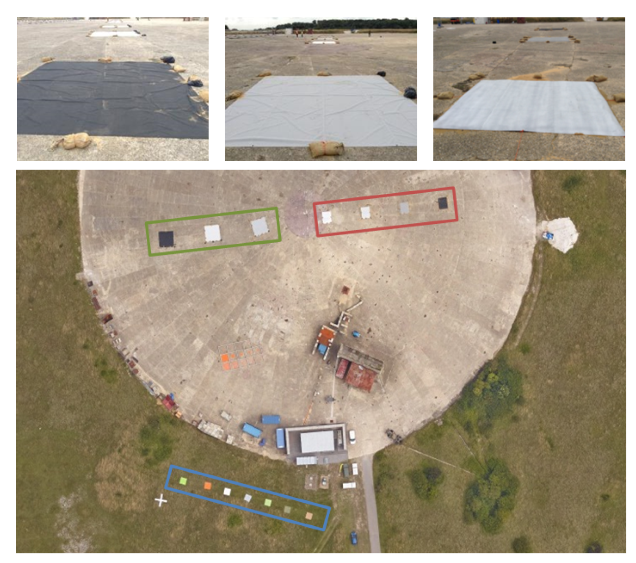A flowchart of the atmospheric search is given in Figure 7. The experimental setup during GT data acquisition and the results of the search algorithm are presented in Section 7.

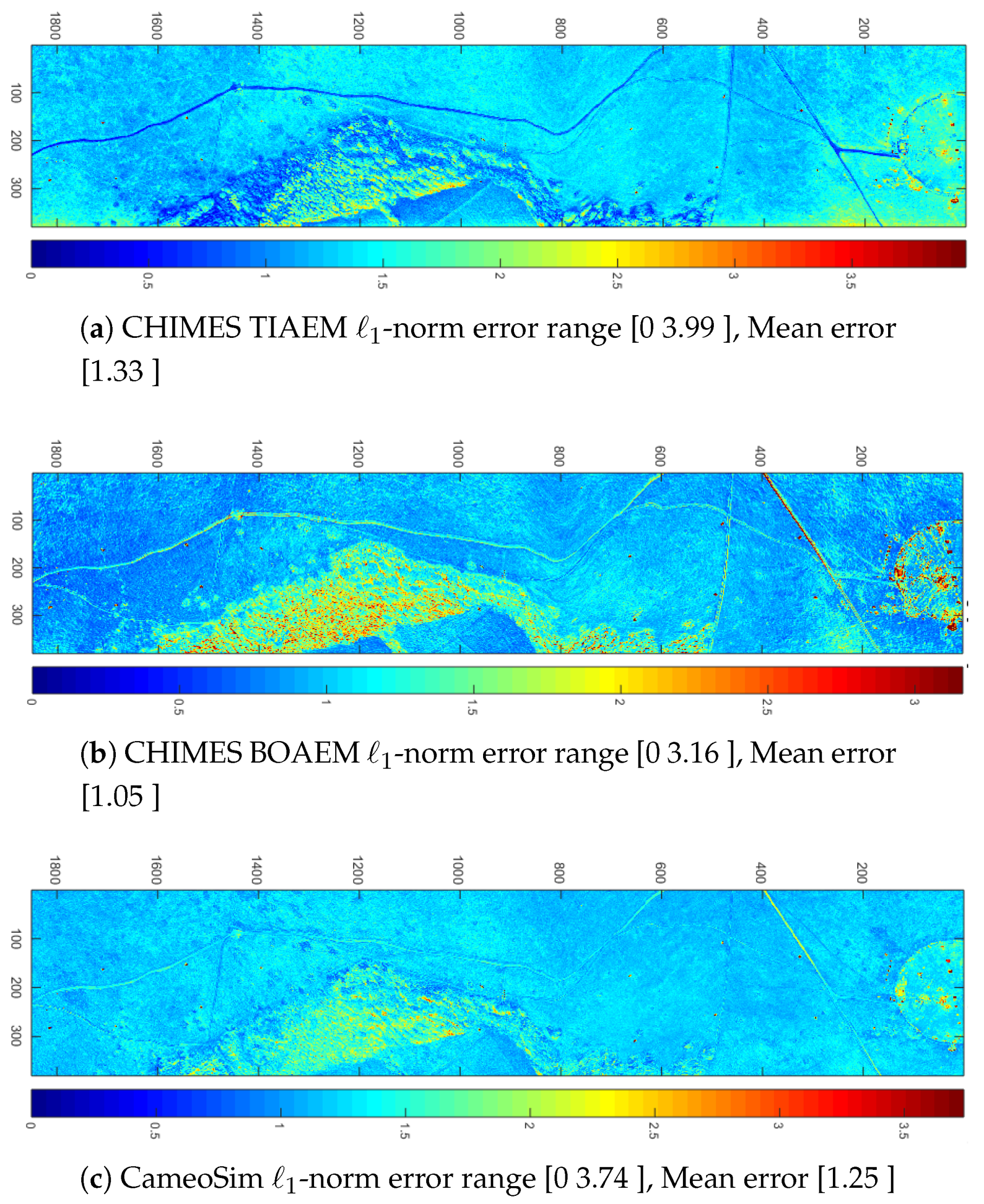
In this section, we discussed adjacency models included in CHIMES. Concisely, the BOAEM is a simplistic adjacency model which evaluates the upwelling by using one spectral reflectance. Other simulators such as the CameoSim has also employed a similar model for adjacency modelling. However, the TIAEM may represent a more comprehensive adjacency model in which it evaluates the local adjacency in upwelling radiance within several small ROIs across the entire scene.

4. Components of CHIMES

4.1. Scene

The terrain is generated by DEM-based smoothed deformation in the flat polygon, which is the basic primitive of a scene. The input data is airborne reflectance images with the high spatial and spectral resolution, which is processed by QUAC atmospheric compensation on radiance image. Classification of reflectance image cube is the first step for material mapping, which is performed by K-means clustering algorithm with a user-defined number of materials (classes) input. Details about classified texture are covered in a subsequent section. The number of specified material and their identifiers are created and stored in the database. A texture is generated based on materials RGB colours. An identifier based coded-texture layer is generated to handle the loading of spectral data during rendering. Corresponding BRDF/BTDF is associated with each material, however, the thermal description is out of the scope of this work. This classified texture is mapped onto the terrain to create static geometry. A potentially roving geometry as shown in Figure 1 might be represented by vehicles, plumes or clouds, however, it is not included in this version of the simulator.

In terms of rendering system, a scene is an input to the rendering algorithm which recursively cast rays to test occlusion for casting shadows or perform an interaction with scene surface to determine the ray response according to reflection or transmission distribution functions. Another important interaction of the scene is with the sensor, the orientation, altitude and azimuth of the sensor create a perception of the scene on the sensor. Although the skydome itself is not part of scene geometry, however, it may include substantial space in an outdoor scene, viewed by the sensor.

Classified Texture

In our experiments, K-means clustering is employed for classification, which is performed on an atmospherically compensated (by QUAC [38]) reflectance hyperspectral cube. In this phase of research where the focus is on RT models, classification from MSI or RGB image like CameoSim/DIRSIG is out of the scope. K-means clustering requires a user-defined number of classes as input. RGB image of classification from 80 and 120 classes are shown in Figure 8a,b, respectively. These classification results are performed in Matlab GPU based implementation using 100 K iterations.

A flat polygon is transformed into the terrain by introducing DEM driven realistic bumps onto it. DEM is measured in Absolute Ground Level (AGL) for the test scene and it is shown in Figure 9a. The classified image from Figure 8b is mapped on the terrain to construct a classified texture, as shown in Figure 9b.

4.2. Sensor

Radiance generated by MODTRAN has a very high spectral resolution ranging from wavenumbers ($\tilde{\nu }$) between 3800 to 28000 (cm${}^{-1}$). To simulate a real sensor the output is spectrally degraded to represent the instrument characteristic spectral channels. This is achieved by means of convolution with sensor response functions. The normalised convolved radiance values in band i are calculated as;

$$L_{si}=\frac{{\displaystyle {\int }_{\lambda }{L}_{mi}\left(\lambda \right)r_i\left(\lambda \right)d\lambda }}{{\displaystyle {\int }_{\lambda }{r}_i\left(\lambda \right)d\lambda }},$$

(26)

where $L_{si}$ is convolved radiance of ith band, $L_{mi}$ is MODTRAN high spectral resolution radiance and $r_i$ is the response function in ith band [39].The sensor module also takes part in the rendering system by accepting the samples and returning rays distributed on the detector’s view grid, whose count is defined by the user as rays per pixel. A scene is visible to the view grid by depth-sensitive perspective projections.

5. Additional Enhanced Features in CHIMES

5.1. Polarised Skydome Radiance

Although MODTRAN has provided irradiance models for the emitters such as the sun, moon [40], in CHIMES the sun and sky irradiance have been implemented as a skydome which is generated through interpolation of MODTRAN’s look-up table (LUT) for various zenith and azimuth settings. MODTRAN is typically run with multiple scattering models (DISORT scaled Isaac) and Mie scattering for the appropriate atmosphere (aerosols) of the scene given by the atmospheric search algorithm as described in Section 3.2. A skydome degree of polarisation (DOP) is achieved by rayleigh scattering on environment maps pixel position (zenith, azimuth) with respect to solar position, polarimetric version of MODTRAN called MODTRAN-P [24] is not used to generate this skydome. The sensor response is convolved with the MODTRAN radiance as described in Section 4.2. Figure 10a, plots the variation of radiance for skydome with clouds, while Figure 10b shows the DOP of the sky for depicted (by yellow circle) solar azimuth and zenith positions. It is seen from these figures that a strong polarization of solar irradiance is observed at $90$° with respect to solar vector and is caused by the Rayleigh scattering of the air molecules in the atmosphere [41]. It should be noted that clouds are not added as roving geometry in this version of CHIMES, however reduced radiance due to presence of cloud is calculated from MODTRAN and skydome with lower radiance is created. A polar plot of skydome radiance in overcast weather is shown in Figure 11a. A similar plot for clear sky, that is, with no aerosol is shown in Figure 11b.

5.2. Rendering

Rendering is the key component of the CHIMES simulator. The light-transport scheme employed in rendering path tracing. A more detailed text about this rendering scheme may be found in Reference [42]. Each pixel in the sensor plane is sampled by Poisson sampling and variable number of rays can be defined in parameters. Increasing number of rays increases rendering time but provide higher image quality. Multiple importance sampling [36] is applied for direct light source with BRDF/BTDF and diffuse light source with phase function. The phase function employed during rendering is Henyey-Greenstein function. Rendering is a recursive operation which is repeated for a user-defined ray bounce. A scene is divided into blocks where each block is rendered in parallel. The eventually accumulated radiance for each pixel is computed which is passed to the image reconstruction component. The image reconstruction component estimates the pixel intensity based on radiance and applies anti-aliasing filter, together with texture interpolation.

6. Experiment

6.1. Experimental Data

For experimental validation, we have a reference airborne HSI scene called Selene SCIH23 dataset [43] which was acquired by the Defence Science and Technology Laboratory (DSTL) covering 0.4 to $2.5$ $\mathsf{\mu }$$\mathrm{m}$. DEM of this scene was also captured by LIDAR (Light Detection And Ranging) which is shown in Figure 9a. It is a registered image which is separately taken from HySpex VNIR-1600 (160 bands between 0.414–0.975 $\mathsf{\mu }$m) and SWIR-384 (288 bands between 0.978–2.509 $\mathsf{\mu }$m) sensors mounted on the same airborne platform at altitude of 944 meters. This scene was acquired near Salisbury, UK, on 12 August 2014 BST 13:00:04. The registered image has a GSD of 70 × 70 cm, QUAC was applied using ENVI software for atmospheric compensation. This scene has several planted calibration panels, tiles, carpets and perspex, having both full and sub-pixel sizes. RGB images of Selene scene is shown in Figure 12, which also contains ROI markings, used in Section 7.

6.2. Experimental Setup Employed in Automatic Search for Atmospheric Parameters

The Selene scene is a vegetation biased scene, however, several fabric calibration panels with known reflectance are planted across the scene as shown in Figure 13. A white calibration panel with an average reflectivity of 99.0% and a black panel with average reflectivity of 2.0% are selected as reference materials. Moreover, there are seven large fabric panels with particular spectral properties were placed to act as calibration targets and deployed across the centre of the Hard Target (concrete) [43]. Figure 13 shows both ground (first row) and aerial (second row) image of the scene. Aerial image marks regions where some panels and tiles are planted.

7. Results and Validation

Simulation results are assessed based on variable terrain types, atmosphere types and adjacency models as discussed in Section 3.1. Summarized results for each of these parameters are included subsequently, however, more detailed material-wise statistical analysis is included in Appendix A. Error metrics used for evaluation are defined in Appendix B.

We report the results of the search algorithm for atmospheric parameterization in the subsequent section, followed by results of simulations. In atmosphere search we observe a closer match between white panel’s radiance and MODTRAN’s $L_w$, however relatively larger error for MODTRAN’s path radiance $L_b$ and black panel’s radiance. In simulation results, we observe a closer match between CHIMES BOAEM and CameoSim under cloudy atmosphere and flat terrain, in terms of radiance error ranges and patterns. Moreover, the material wise results in Appendix A also shows a closer agreement between CHIMES (BOAEM) and CameoSim. It is shown in the appendix that TIAEM produces better spectral reflectance shapes (colours) for the man-made target materials, particularly in the VNIR region. In the case of a clear sky, all models produce similar results.

7.1. Automatic Search for Atmospheric Parameters

During the search process, MODTRAN is input with several parameters, few of them are shown in Table 5. In our experimental data, sensor altitude is higher than cloud base and presence of thin cloud below the sensor is also reported [43], therefore we will vary the aerosol optical thickness below the sensor to search the approximate underlying atmospheric condition in the scene.

In each iteration MODTRAN’s $L_w$ that is, accumulated total ground reflected radiance and path radiance is calculated and goodness of fit is recorded. Estimate of searched white panel radiance $L_w$ and black panel radiance $L_b$ is shown in Figure 14, that possesses the highest goodness of fit, that is 90.4% of match in terms of NRMSE for $L_w$ and 55.26% for $L_b$, respectively. These results manifest good atmospheric search in terms of total ground reflected radiance, however, estimation of path radiance is relatively worse. If path radiance estimated in the search process is lower than the GT panel then it may result in higher contrast than the GT. As the search method only employs MODTRAN at-sensor radiance estimate, the effect of volumetric scattering is not accounted for. At rendering time, volumetric scattering may either reduce the error in the estimate of $L_b$ or increase it depending on the choice of phase function and backscattering parameter, such as the variable g in Henyey-Greenstein function [42]. However, due to good estimation of the TGRR, we have selected searched parameters ($C_w$ = 0.22 gm/m${}^3$ and R = 0.024 Km) and fixed parameters given in Table 5 for our overcast condition simulations. In the case of atmospheric search by using white and black panel, it is easier to segregate the path radiance and TGRR, therefore these targets were employed. A similar search based on orange perspex yielded ($C_w$ = 0.22 gm/m${}^3$ and R = 0.023 Km), which is very close to white and black panel’s parameters.

7.2. CHIMES and CameoSim Simulation Results with Flat Terrain

RGB images of Selene scene rendered by CHIMES and CameoSim are shown in Figure 15. Inputs and parameters to both simulators are the same, particularly the atmospheric condition is cloudy with parameters shown in Table 5 and the scene geometry is flat terrain. We observe illumination differences in the RGB images, particularly at the region having trees, closer to the farm. It should be noted that the region with trees and buildings on the concrete hard target show a higher error. The scene posses both trough and crest bumps which cause a higher error. Another contributing factor that accumulates the error, is the presence of shadows [44]. As shown in Figure 16b,c, CHIMES BOAEM and CameoSim, apparently have closer ${\ell }_1$-norm error, the error map also shows a closer error range and mean error, compared to TIAEM. The error range of BOAEM is between 0–3.16 with a mean error of 1.05. CameoSim error lies in the range of 0–3.74 with a mean error of 1.25. The visual pattern of the error map does look similar to discrepancies in the tree region in CHIMES BOAEM which has high error relative to CameoSim. On the other hand CHIMES TIAEM error map has a higher range, lying between 0–3.99 with a mean error of 1.33. All three error maps have higher error in tree, building and low reflectance target regions.

Several ROIs are considered for evaluating the mean of radiance across the scene, these ROIs are shown in Figure 12. Selection of these ROIs is biased towards vegetation which constitutes more than 80% of the scene. As mentioned in Section 1, the rationale behind this ROI selection is in the evaluation of background statistic of models. Out of this eight, seven are grass, while one is from the concrete hard target. Mean spectral radiance of these ROIs is shown in Figure 17. NRMSE and ${\ell }_1$-norm errors are tabulated in

Table 6. NRMSE, ${\ell }_1$-norm error of radiance in Figure 17. Material of ROI 2 is concrete, other ROIs are grass across the scene. Least errors are shown in bold text.

ROI	Error	CHIMES TIAEM	CHIMES BOAEM	CameoSim
ROI 1	NRMSE	29.9207%	17.602%	24.822%
	${\ell }_1$-norm	1.3772	0.921	1.211
ROI 2	NRMSE	30.187%	19.455%	22.871%
	${\ell }_1$-norm	1.637	1.107	1.270
ROI 3	NRMSE	25.970%	17.250%	22.059%
	${\ell }_1$-norm	1.3839	1.010	1.234
ROI 4	NRMSE	29.436%	16.736%	26.695%
	${\ell }_1$-norm	1.255	0.774	1.163
ROI 5	NRMSE	25.476%	16.904%	21.673%
	${\ell }_1$-norm	1.325	0.959	1.172
ROI 6	NRMSE	29.901%	17.575%	24.417%
	${\ell }_1$-norm	1.255	0.930	1.255
ROI 7	NRMSE	27.547%	17.483%	23.101%
	${\ell }_1$-norm	1.428	1.010	1.269
ROI 8	NRMSE	31.918%	20.771%	22.313%
	${\ell }_1$-norm	1.673	1.215	1.275

, which shows that CHIMES BOAEM has consistently lower errors compared to TIAEM and CameoSim.

Similarly, man made material radiance shown in Appendix A also show closer match between BOAEM and CameoSim in terms of NRMSE error of mean radiance.

Eigenanalysis is also performed for evaluation of results. Eigenvectors of band to band covariance matrix are calculated. A NRMSE error between first four eigenvectors with respect to GT is shown in Figure 18. As the trend developed in a previous error metric, both BOAEM and CameoSim have similar NRMSE error magnitude. It should be noted that TIAEM has substantially lower error magnitude in first eigenvector. This trend also apparent in material wise eigenanalysis shown in Appendix A.

For example, TIAEM has 18.3% NRMSE compare to 79.4% and 73.4% of BOAEM and CameoSim, respectively, for first eigenvector. In the next two eigenvectors BOAEM has the lowest error magnitude, while CameoSim has the lowest error in the last one. In case of material wise radiance analysis presented in Appendix A, CHIMES TIAEM and BOAEM have the lower NRMSE error with respect to GT compared to CameoSim. For example in orange perspex near grass TIAEM has an error of 13.2%, while CHIMES BOAEM has an error of 8.8%, compared to CameoSim’s 89.9%.For concrete, TIAEM has the error magnitude of 28.0% compared to BOAEM’s 26.8% and CameoSim’s 25.5%. Therefore CameoSim performs slightly better for concrete, in terms of eigenvector matching with GT.

Figure A1 and Figure A2 clearly show influence of albedo material that is, grass scrub in VNIR region in BOAEM and CS results. However, TIAEM does not depict this over influence of the average background albedo material used in MODTRAN calculations. Even though TIAEM still cause increase in radiance at high albedo bands. Similarly this trend is visible in the DEM based results as well.

7.3. CHIMES and CameoSim Simulation Results with DEM

Rugged terrain causes a non unity sky-view factor, which attributes to inclusion of background reflection and reduced diffuse radiance. It is therefore important to validate the differences in radiance with and without terrain. RGB images of simulated scene with DEM surface is shown in Figure 19. In case of RGB channels, we observe that in contrary to results of flat terrain, the contrast in both models of CHIMES images has substantially reduced, particularly in the region where terrain is higher. This manifests the background contribution due to reflection. In CameoSim image we observe reduced spatial reconstruction quality leading to apparent pixelation. However, the visual contrast appears to increase in CameoSim compared to the flat terrain simulation. A more clearer picture about error is found in ${\ell }_1$-norm error map in Figure 20, subsequently.

Figure 20 shows that CHIMES TIAEM has an error range of 0–4.13, with the mean error of 1.38 compared to 0–3.99, with the mean error of 1.33, in case of flat terrain. The increase in mean error is therefore 3.6 %. Simlarly, CHIMES BOAEM has an error range of 0-3.28, with the mean error of 1.09 compared to 0–3.16, with the mean error of 1.05, in case of flat terrain. The increase in mean error in this case is 3.7%. For CameoSim result, the error range is 0–18.33, with the mean error of 6.11 compared to 0–3.74, with the mean error of 1.25 for flat terrain. The increase in error is 388.8%. The relative pattern of error as shown Figure 20 is similar to that in flat terrain case.

We present the ROI based mean radiance magnitude like presented in flat terrain case. The radiance is increased in all simulations due to background reflected contributions. Figure 21 and

Table 7. NRMSE, ${\ell }_1$-norm error of radiance in Figure 21. Material of ROI 2 is concrete, other ROIs are grass across the scene. Least errors are shown in bold text.

ROI	Error	CHIMES TIAEM	CHIMES BOAEM	CameoSim
ROI 1	NRMSE	27.510%	16.980%	118.307%
	${\ell }_1$-norm	1.338	0.913	6.160
ROI 2	NRMSE	29.793%	17.806%	112.323%
	${\ell }_1$-norm	1.651	0.979	5.997
ROI 3	NRMSE	25.040%	16.955%	96.663%
	${\ell }_1$-norm	1.365	1.001	5.901
ROI 4	NRMSE	28.456%	17.235%	134.023%
	${\ell }_1$-norm	1.248	0.816	6.341
ROI 5	NRMSE	24.896%	16.621%	99.948%
	${\ell }_1$-norm	1.316	0.944	5.951
ROI 6	NRMSE	28.253%	18.353%	116.072%
	${\ell }_1$-norm	1.436	1.006	6.092
ROI 7	NRMSE	26.090%	17.259%	101.742%
	${\ell }_1$-norm	1.426	1.014	5.916
ROI 8	NRMSE	30.925%	19.874%	91.241%
	${\ell }_1$-norm	1.661	1.184	5.724

show that CHIMES BOAEM has the least NRMSE and ${\ell }_1$ Norm error in almost all ROIs. It is encouraging to note that CHIMES BOAEM’s error reduced for all eight ROIs when DEM is introduced. CHIMES TIAEM however maintains similar error as in flat terrain case. The CameoSim result for ROIs shows an enormous increase in errors.

Similar to flat terrain, eigenvectors for the DEM are also calculated. Eigenvectors’ plot is shown in Figure 22.The NRMSE error in this case observe an increase in simulated results. For example, TIAEM has 44.2% NRMSE compared to 72.6% and 53.4% of BOAEM and CameoSim, respectively, for the first eigenvector. Similar to flat terrain, in the second two eigenvectors BOAEM has the lowest error magnitude. The error magnitude of all simulation results exceed 100% in third and fourth eigenvector cases.

7.4. CHIMES and CameoSim Simulation Results with Clearsky

We have briefly included the results of a simulation in a clearsky atmosphere. There are no aerosols and clouds in these simulations. This is a scenario where scattering has little affect therefore adjacency effect should not be observed. Lack of aerosol increases transmission and therefore the at-sensor radiance magnitude is higher. We include ${\ell }_1$-norm error map and radiance of white panel to show a comparison of simulations.

Due to the lack of adjacency effect, a closer match between CHIMES TIAEM and BOAEM models is expected. It is premised by the ${\ell }_1$-norm error map shown in Figure 23. Although we calculate ${\ell }_1$-norm error with respect to ground truth, however as the atmosphere is far from the true scene’s atmosphere, therefore error magnitude have no significance. GT is only used as a reference radiance to show similarity between the simulation models. In ${\ell }_1$-norm error CHIMES TIAEM has an error range of 0–12.79, with the mean error of 4.28. CHIMES BOAEM has an error range of 0–12.70, with the mean error of 4.23. CameoSim’s error is in range 0–14.71, with the mean error of 4.90, as shown Figure 23. We observe a close match in error ranges, mean error and error pattern across the scene.

Radiance from ROI of white panel is shown in Figure 24. Both magnitude and signature of output radiance for all simulation models look in close agreement with each other.

8. Discussion

8.1. Variable Atmospheric Condition

In a clear-sky atmosphere, MODTRAN’s predefined "no-aerosol" setting is used. Clearsky simulation results show that both models of CHIMES produce similar results compared to CameoSim. The ${\ell }_1$-norm error range for the whole scene simulated with TIAEM and BOAEM the error ranges are between 0–12.79 and 0–12.70 with the mean error of 4.28 and 4.23, respectively. In the case of CameoSim simulation the range of ${\ell }_1$-norm error is between 0 and 14.71 with a mean error of 4.90. In terms of rendering the coupling of ray tracer with phase function is relatively insignificant because of lower scattering coefficients in this atmosphere. On the other hand coupling of the ray-tracer direct emitter with target reflectance, BRDF is more dominant which manifests the fact that all models are working similarly when direct light is dominant and atmosphere has lower scattering efficiency. In clear-sky simulations, flat terrain was used. Results of overcast condition are covered in subsequent sections, for flat and DEM terrains.

8.2. Flat Terrain

When simulations were performed with flat terrain, CHIMES TIAEM simulated image has ${\ell }_1$-norm error for the whole scene in the range of 0–3.99 with the mean error of 1.33, compared to CHIMES BOAEMs 0–3.16 with the mean error of 1.05. CameoSim’s ${\ell }_1$-norm error range lies between 0–3.74 with a mean error of 1.25. Therefore CHIMES BOAEM model is the best performer, while TIAEM is the worst in terms of ${\ell }_1$-norm error, which might be a consequence of higher textural variation during volumetric scattering. On the other hand, if we compare the eigenvectors of the covariance matrix of the simulated scenes, TIAEM’s first vectors have minimum 18% NRMSE compared to BOAEMs 79.4% and CameoSims 73.4%, with respect to the ground truth. Better estimation of covariance statistics of a scene signifies better estimation of detector performance through a simulated scene. These target detectors include Adaptive Cosine Estimator (ACE) and Match Filter and so forth, that depends upon HSI image’s band to the band covariance matrix. If a simulator generates good statistics of the scene for variable conditions then target vulnerability can be better assessed.

8.3. DEM–Based Realistic Terrains

When simulations were performed with DEM–based realistic terrain, all three models show an increase in the mean ${\ell }_1$-norm error for the whole image. CHIMES BOAEM still possesses the least mean error of 1.09 with a range of 0–3.28. The TIAEM model’s ${\ell }_1$-norm error lies within 0–4.13 with the mean error of 1.38. CameoSim, on the other hand, shows an unexpected many-fold increase in ${\ell }_1$-norm error compared to both models of CHIMES. As CameoSim is a closed software system, it is not possible to verify the cause of increase error in CameoSim. However, as mentioned in the text the sky-view factor, in this case, becomes less than 1.0, causing non-zero contribution of background reflected radiance.

9. Conclusions

In this paper, we introduced a new end-to-end Hyperspectral Image generation system, which generates HSI image in the visible to SWIR region of the electromagnetic spectrum. The image simulated in this work was taken by Hyspex dual VNIR1600 and SWIR384 cameras. Our simulator creates a skydome from MODTRAN radiance and employs path tracing based light transport for calculating the at-sensor radiance. It also incorporates Digital Elevation Models to generate the relatively rugged surface. We also presented a method to search for atmospheric parameters, given a known reflectance material in the scene.

In this research, we were primarily focused on implementing and evaluating alternate adjacency models. We introduced an adjacency effect model which uses one average background spectra for the whole scene (BOAEM), we also proposed localized background spectra retrieved from neighbouring texture pixels (TIAEM). Both of our models employ volumetric backscattering builtin the renderer. We compared results of both these models with CameoSim and Ground Truth.

Imagery generated by CHIMES using BOAEM model shows close agreement with CameoSim. The CHIMES TIAEM model shows deviation from both BOAEM and CameoSim results and yields a higher error in flat scene geometry, however, it consistently performed better in eigenanalysis of the whole imagery, particularly in first eigenvectors of both flat and DEM terrains. Moreover, analysis of target material in Appendix A shows that the shape of radiance generated by CHIMES TIAEM matches closely in VNIR region. It is noted during the analysis that CHIMES-BOAEM came out to have the least error as shown in Table 6, it even showed a slump in error when rugged terrain is used, as shown in Table 7. This DEM data represent the real height-map of the scene when it was captured.

CameoSim generated imagery in flat terrain stands second in terms of least error with respect to ground truth, as shown in Table 6. However, when DEM is introduced in terrain, the error leapt up by several times as shown in Figure 20 and Table 7. Selene scene has some regions consisting tall tree, however, it is essentially a flat scene otherwise. An increase in error to this extent was therefore not expected.

References

1. Stamnes, K.; Tsay, S.C.; Wiscombe, W.; Jayaweera, K. Numerically stable algorithm for discrete-ordinate-method radiative transfer in multiple scattering and emitting layered media. Appl. Opt. 1988, 27, 2502–2509. [Google Scholar] [CrossRef] [PubMed]
2. Kerkes, J.P. Introduction to FASSP and List of Related Publications. 2005. Available online: http://www.cis.rit.edu/people/faculty/kerekes/fassp.html (accessed on 6 October 2019).
3. Kerekes, J.P.; Baum, J.E. Full-spectrum spectral imaging system analytical model. IEEE Trans. Geosci. Remote Sens. 2005, 43, 571–580. [Google Scholar] [CrossRef]
4. Schott, J.R. Remote Sensing: The Image Chain Approach, 2nd ed.; Oxford University Press: Madison Avenue, NY, USA, 2007. [Google Scholar]
5. Schott, J.; Brown, S.; Raqueño, R.; Gross, H.; Robinson, G. An Advanced Synthetic Image Generation Model and its Application to Multi/Hyperspectral Algorithm Development. Can. J. Remote Sens. 1999, 25, 99–111. [Google Scholar] [CrossRef]
6. Ientilucci, E.J.; Brown, S.D. Advances in wide-area hyperspectral image simulation. In Targets and Backgrounds IX Characterization and Representation; Watkins, W.R., Clement, D., Reynolds, W.R., Eds.; International Society for Optics and Photonics, SPIE Press: Bellingham, WA, USA, 2003; Volume 5075, pp. 110–121. [Google Scholar] [CrossRef]
7. Ientilucci, E.J. Synthetic Simulation and Modeling of Image Intensified CCDs (IICCD); Technical Report; Rochester Institute of Technology: Rochester, NY, USA, 1996. [Google Scholar]
8. Goodenough, A.A.; Brown, S.D. DIRSIG5: Next-Generation Remote Sensing Data and Image Simulation Framework. IEEE J. Sel. Top. Appl. Earth Obs. Remote Sens. 2017, 10, 4818–4833. [Google Scholar] [CrossRef]
9. Berk, A.; Conforti, P.; Kennett, R.; Perkins, T.; Hawes, F.; van den Bosch, J. MODTRAN6: A major upgrade of the MODTRAN radiative transfer code. In Algorithms and Technologies for Multispectral, Hyperspectral, and Ultraspectral Imagery XX; Velez-Reyes, M., Kruse, F.A., Eds.; International Society for Optics and Photonics, SPIE Press: Bellingham, WA, USA, 2014; Volume 9088, pp. 113–119. [Google Scholar] [CrossRef]
10. Brady, A.; Kharabash, S. Further Studies into Synthetic Image Generation using CameoSim; Technical Report; Defence Science and Technology Organisation: Edinburgh, South Australia, 2011.
11. Moorhead, I.R.; Gilmore, M.A.; Houlbrook, A.W.; Oxford, D.E.; Filbee, D.R.; Stroud, C.A.; Hutchings, G.; Kirk, A. CAMEO-SIM: A physics-based broadband scene simulation tool for assessment of camouflage, concealment, and deception methodologies. Opt. Eng. 2001, 40, 1896–1905. [Google Scholar] [CrossRef]
12. Nelsson, C.; Hermansson, P.; Winzell, T.; Sjökvist, S. Benchmarking and Validation of IR Signature Programs: SensorVision, CAMEO-SIM and RadThermIR; Technical Report; Swedish Defence Research Agency: Linkoping, Sweden, 2005.
13. Willers, C.J.; Willers, M.S.; Lapierre, F. Signature modelling and radiometric rendering equations in infrared scene simulation systems. In Technologies for Optical Countermeasures VIII; Titterton, D.H., Richardson, M.A., Eds.; International Society for Optics and Photonics, SPIE Press: Bellingham, WA, USA, 2011; Volume 8187, pp. 173–188. [Google Scholar] [CrossRef]
14. Willers, M.S.; Willers, C.J. Key considerations in infrared simulations of the missile-aircraft engagement. In Technologies for Optical Countermeasures IX; Titterton, D.H., Richardson, M.A., Eds.; International Society for Optics and Photonics, SPIE Press: Bellingham, WA, USA, 2012; Volume 8543, pp. 180–195. [Google Scholar] [CrossRef]
15. Willers, C.J. Electro-Optical System Analysis and Design: A Radiometry Perspective; SPIE Press: Bellingham, WA, USA, 2013. [Google Scholar] [CrossRef]
16. Willers, C.J.; Willers, M.S.; de Waal, A. Aircraft vulnerability analysis by modeling and simulation. In Technologies for Optical Countermeasures XI; and High-Power Lasers 2014: Technology and Systems; Titterton, D.H., Richardson, M.A., Grasso, R.J., Bohn, W.L., Ackermann, H., Eds.; International Society for Optics and Photonics, SPIE Press: Bellingham, WA, USA, 2014; Volume 9251, pp. 151–166. [Google Scholar] [CrossRef]
17. Sundberg, R.L.; Richtsmeier, S.; Haren, R. Full optical spectrum hyperspectral scene simulation. In Proceedings of the 2005 IEEE International Geoscience and Remote Sensing Symposium (IGARSS ’05), Seoul, Korea, 25–29 July 2005; Volume 5, pp. 3235–3238. [Google Scholar] [CrossRef] [Green Version]
18. Sundberg, R.; Richtsmeier, S.; Berk, A.; Adler-Golden, S.M.; Fox, M.J.; Haren, R. Thermal Infrared Scene Simulation for Plume Detection Algorithm Evaluation; SPIE Defense + Commercial Sensing; SPIE Press: Bellingham, WA, USA, 2004. [Google Scholar]
19. Pereira, W.; Richtsmeier, S.; Carr, S.; Kharabash, S.; Brady, A. A comparison of MCScene and CameoSim simulations of a real scene. In Proceedings of the 2014 6th Workshop on Hyperspectral Image and Signal Processing: Evolution in Remote Sensing (WHISPERS), Lausanne, Switzerland, 24–27 June 2014; pp. 1–4. [Google Scholar] [CrossRef]
20. Hawes, F.T.; Berk, A.; Richtsmeier, S.C. Development and validation of P-MODTRAN7 and P-MCScene, 1D and 3D polarimetric radiative transfer models. In Polarization: Measurement, Analysis, and Remote Sensing XII; Chenault, D.B., Goldstein, D.H., Eds.; International Society for Optics and Photonics, SPIE Press: Bellingham, WA, USA, 2016; Volume 9853, pp. 215–221. [Google Scholar] [CrossRef]
21. Cota, S.A.; Bell, J.T.; Boucher, R.H.; Dutton, T.E.; Florio, C.J.; Franz, G.A.; Grycewicz, T.J.; Kalman, L.S.; Keller, R.A.; Lomheim, T.S.; et al. PICASSO: An end-to-end image simulation tool for space and airborne imaging systems. J. Appl. Remote Sens. 2010, 4, 1–37. [Google Scholar] [CrossRef]
22. Cota, S.A.; Lomheim, T.S.; Florio, C.J.; Harbold, J.M.; Muto, B.M.; Schoolar, R.B.; Wintz, D.T.; Keller, R.A. PICASSO: An end-to-end image simulation tool for space and airborne imaging systems II. Extension to the thermal infrared: Equations and methods. In Imaging Spectrometry XVI; Shen, S.S., Lewis, P.E., Eds.; International Society for Optics and Photonics, SPIE Press: Bellingham, WA, USA, 2011; Volume 8158, pp. 160–184. [Google Scholar] [CrossRef]
23. Guanter, L.; Segl, K.; Kaufmann, H. Simulation of Optical Remote-Sensing Scenes With Application to the EnMAP Hyperspectral Mission. IEEE Trans. Geosci. Remote Sens. 2009, 47, 2340–2351. [Google Scholar] [CrossRef]
24. Schott, J.R. Fundamentals of Polarimetric Remote Sensing; SPIE Press: Bellingham, WA, USA, 2009. [Google Scholar] [CrossRef] [Green Version]
25. Nicodemus, F.E. Directional Reflectance and Emissivity of an Opaque Surface. Appl. Opt. 1965, 4, 767–775. [Google Scholar] [CrossRef]
26. Schott, J. Remote Sensing, The Image Chain Approach, 1st ed.; Oxford University Press: Madison Avenue, NY, USA, 1997; pp. 80–92. [Google Scholar]
27. Dobbs, B. The Incorporation of Atmospheric Variability into DIRSIG; Technical Report; Rochester Institute of Technology: Rochester, NY, USA, 2006; Available online: http://scholarworks.rit.edu/theses/3011 (accessed on 6 October 2019).
28. Berk, G.A.; Acharya, P. Modtran 5.3.2 User’s Manual; Spectral Sciences, Inc.: Burlington, MA, USA, 2013. [Google Scholar]
29. Goodenough, A.A. Discussion of Requirements for External Atmospheric Data and Models. 2016. Available online: http://www.dirsig.org/download/AtmTransMeeting2016/DIRSIG5_AtmTrans_2016.pptx.pdf (accessed on 6 October 2019).
30. Richter, R. Atmospheric/Topgraphic Correction for Airborne Imagery (ATCOR4 User Guide). 2016. Available online: http://www.rese.ch/pdf/atcor4_manual.pdf (accessed on 6 October 2019).
31. Ma, J.; Li, X.; Chen, X.; Feng, C. Target adjacency effect estimation using ground spectrum measurement and Landsat-5 Satellite data. IEEE Trans. Geosci. Remote Sens. 2006, 44, 729–735. [Google Scholar] [CrossRef]
32. Richter, R.; Martin Bachmann, W.D.; Müller, A. Influence of the Adjacency Effect on Ground Reflectance Measurements. IEEE Geosci. Remote Sens. Lett. 2006, 3, 1–12. [Google Scholar] [CrossRef]
33. Tanre, D.; Herman, M.; Deschamps, P.Y. Influence of the background contribution upon space measurements of ground reflectance. Appl. Opt. 1981, 20, 3676–3684. [Google Scholar] [CrossRef] [PubMed]
34. Kaufman, Y.J. The atmospheric effect on the separability of field classes measured from satellites. Remote Sens. Environ. 1985, 18, 21–34. [Google Scholar] [CrossRef]
35. Richter, R. ATCOR Version 4, Software Help Documents. 2016. Available online: https://www.rese-apps.com/software/atcor-4-airborne/index.html (accessed on 7 November 2019).
36. Veach, E. Robust Monte Carlo Methods for Light Transport Simulation. Ph.D. Thesis, Stanford University, Stanford, CA, USA, 1997. [Google Scholar]
37. Kokhanovsky, A. Optical properties of terrestrial clouds. Earth-Sci. Rev. 2004, 64, 189–241. [Google Scholar] [CrossRef]
38. Bernstein, S.; Jin, X.; Gregor, B.; Adler-Golden, S. Quick atmospheric correction code: Algorithm description and recent upgrades. Opt. Eng. 2012, 51, 1–12. [Google Scholar] [CrossRef]
39. Schläpfer, D. MODO: An Interface to MODTRAN4 for the Simulation of Imaging Spectrometry at-Sensor Signals; Rese Applications Schläpfer: Zurich, Switzerland, 2001. [Google Scholar]
40. Fontenla, J.M.; Harder, J.; Livingston, W.; Snow, M.; Woods, T. High-resolution solar spectral irradiance from extreme ultraviolet to far infrared. J. Geophys. Res. Atmos. 2011, 116. [Google Scholar] [CrossRef]
41. Kokhanovsky, A. Optics of Light Scattering Media: Problems and Solutions, 2nd ed.; Springer: London, UK, 2001. [Google Scholar]
42. Pharr, M.; Jakob, W.; Humphreys, G. Physically Based Rendering: From Theory to Implementation; Morgan Kaufmann, Elsevier: Burlington, MA, USA, 2016. [Google Scholar]
43. Piper, J. A new dataset for analysis of hyperspectral target detection performance. In Proceedings of the Hyperspectral Imaging and Applications Conference (HSI 2014), Coventry, UK, 15–16 October 2014. [Google Scholar]
44. Zahidi, U.A.; Chatterjee, A.; Yuen, P.W.T. A Radiative Transfer Model-Based Multi-Layered Regression Learning to Estimate Shadow Map in Hyperspectral Images. Mach. Learn. Knowl. Extr. 2019, 1, 52. [Google Scholar] [CrossRef] [Green Version]
Figure 1. Components of scene simulators.
Remotesensing 12 00074 g001
Figure 2. DIRSIG big equation components [13,26].
Remotesensing 12 00074 g002
Figure 3. CameoSim data flow.
Remotesensing 12 00074 g003
Figure 4. CameoSim-like recursive ray-tracing.
Remotesensing 12 00074 g004
Figure 5. CHIMES Simulator, system level design overview.
Remotesensing 12 00074 g005
Figure 6. (a) Depicts the work flow of the proposed TIAEM model which features the computation of adjacency upwelling through the evaluation of volumetric scattering within terrain and sensor altitude dependent regional region of interest (ROI). (b) Shows an example for the evaluation of the background reflectance of the adjacency pixels (in red) for the test (target) pixel which is in orange/green.
Remotesensing 12 00074 g006
Figure 7. Flowchart for the atmospheric parameters search method.
Remotesensing 12 00074 g007
Figure 8. QUAC is processed on HSI cube to retrieve reflectance cube. K-means clustering is applied to classify this reflectance cube. Classified textures with 80, 120 classes are shown in (a,b).
Remotesensing 12 00074 g008
Figure 9. Terrain with fixed geometry and skydome in CHIMES environment (Pre-spectral rendering RGB view).
Remotesensing 12 00074 g009
Figure 10. CHIMES sky and sun emitters.
Remotesensing 12 00074 g010
Figure 11. CHIMES emitters.
Remotesensing 12 00074 g011
Figure 12. Selene SCIH23 RGB image with ROI marks, used in Section 7.
Remotesensing 12 00074 g012
Figure 13. Commercially available fabric based calibration panels and tiles were planted in Selene scene [43]. Average reflectivity for calibration panels varies from 99.0% to 2.0%.
Remotesensing 12 00074 g013
Figure 14. White and black panel estimates from atmospheric search.
Remotesensing 12 00074 g014
Figure 15. RGB color image for simulated and Ground Truth Selene scene. Atmospheric condition listed in Table 5.
Remotesensing 12 00074 g015
Figure 16. 1 Norm error of simulated scenes with respect to Ground Truth in atmospheric condition of Table 5.
Remotesensing 12 00074 g016
Figure 17. Mean radiance of ROIs shown in Figure 12.
Remotesensing 12 00074 g017
Figure 18. Eigenvectors of covariance of whole simulated and GT scenes. NRMSE of simulated scene Eigenvectors with respect to GT’s.
Remotesensing 12 00074 g018
Figure 19. RGB color image for simulated and Ground Truth Selene scene. Atmospheric condition is given in Table 5.
Remotesensing 12 00074 g019
Figure 20. 1 Norm error of simulated scenes with respect to Ground Truth.
Remotesensing 12 00074 g020
Figure 21. Mean radiance of ROIs shown in Figure 12.
Remotesensing 12 00074 g021
Figure 22. Eigenvectors of covariance of whole simulated and GT scenes. NRMSE of simulated scene Eigenvectors with respect to GTs.
Remotesensing 12 00074 g022
Figure 23. 1 -norm error of simulated scenes with respect to Ground Truth in clear sky atmosphere. GT radiance is only used as reference for calculating error.
Remotesensing 12 00074 g023aRemotesensing 12 00074 g023b
Figure 24. Radiance of white calibration panel in a (5 × 5) ROI. Simulated radiance are for clearsky while ground truth (GT) is under cloudy condition. GT is only used as a reference in this comparison.
Remotesensing 12 00074 g024