Abstract
There have been debates and a lack of understanding about the complex effects of urban-scale urban form on air pollution. Based on the remotely sensed data of 150 cities in the Beijing-Tianjin-Hebei agglomeration in China from 2000 to 2015, we studied the effects of urban form on fine particulate matter (PM2.5) and nitrogen dioxide (NO2) concentrations from multiple perspectives. The panel models show that the elastic coefficients of aggregation index and fractal dimension are the highest among all factors for the whole region. Population density, aggregation index, and fractal dimension have stronger influences on air pollution in small cities, while area size demonstrates the opposite effect. Population density has a stronger impact on medium/high-elevation cities, while night light intensity (NLI), fractal dimension, and area size show the opposite effect. Low road network density can enlarge the influence magnitude of NLI and population density. The results of the linear regression model with multiplicative interactions provide evidence of interactions between population density and NLI or aggregation index. The slope of the line that captures the relationship between NLI on PM2.5 is positive at low levels of population density, flat at medium levels of population density, and negative at high levels of population density. The study results also show that when increasing the population density, the air pollution in a city with low economic and low morphological aggregation degrees will be impacted more greatly.
1. Introduction
In recent years, in addition to tracing emissions from pollution sources and encouraging changes in energy structure, the linkage between urban form and air quality has become a hot topic in the context of global urbanization and urban air pollution, which are some of the largest environmental health threats [1,2]. Urban form, which is characterized by urban scale, density, and development level; layout concentration; border complexity; etc., has a significant impact on the physical ventilation environment, microclimate, and traffic patterns, which then affect the emission and diffusion of air pollutants [3,4,5,6]. Due to the high pressure of urbanization and the lock-in effect of urban form worldwide, it has become an urgent international issue to gain insight into the complex relationship between urban form and air pollution from multiple perspectives.
Remarkable research progress has been made on the relationship between urban form and air pollution, but it has not solved the long-standing debates [7]. Most studies have found that larger cities worsen air quality, while some studies did not find any relationship [8]. Moreover, there is more inconsistent evidence from empirical research conducted around the world. A study of 45 metropolitan areas in the United States showed that the increase in urban density can reduce NO2 emissions by controlling the factors of population size and temperature [6]. Another study of 111 cities in the United States showed that higher population density (POPDEN) led to higher FINE particulate matter (PM2.5) concentration and air quality index (AQI) values per capita [9]. A study of 83 cities around the world showed that the decrease in NO2 caused by a 4% increase in urban continuity can offset the negative impact of a 10% increase in population size [10,11]. However, another study based on 157 urban samples in China showed that higher urban continuity can worsen air quality [12]. More inconsistencies can be found in studies around the world [7].
On the one hand, the high density and high compactness of urban form enable residents to obtain living services and work opportunities nearby, reducing the separation of work and residence, change the means of transportation, reduce the use of private cars, promote public transport travel, and thus reduce the emission of air pollutants [13,14]. On the other hand, the increase of POPDEN may lead to more traffic flow, more energy consumption burden on the transportation system, and more traffic congestion, which will worsen air quality [15,16,17]. The high-density buildings in high population density cities often lead to deeper and more closed urban canyons, which reduce the efficiency of air pollutant diffusion from canyons to the atmosphere and cause pollution accumulation [13,18,19]. These positive or negative effects are further influenced by geographical and climatic conditions as well as urban fundamental characteristics, showing different comprehensive effects in different regions and spatial scales.
Moreover, the conflicting conclusions are also caused by the use of different statistical models (panel or cross-section regression) at different scales (global scale, regional scale, and case scale). Another major obstacle to gaining deeper insights is that the existing research still lacks careful consideration of the nonlinear relationship between urban form and air pollution, which may be derived from the interactions among urban forms. The interaction between these urban morphology factors has been proven to have an important impact on the urban environment [20]. The interactions among urban form indicators imply that the influence of each of them on the urban environment cannot be separated. However, these considerations are still lacking in the study of the relationship between urban form and air pollution, which will hinder the adjustment of planning strategies for cleaner air and sustainability.
To resolve these knowledge gaps, based on remote sensing inversion data, we included 150 cities of the Beijing-Tianjin-Hebei urban agglomeration in China as the research samples to conduct an empirical study about the impacts of urban density, development level, aggregation index (AI) and fractal dimension (FRAC) on the concentrations of two urban pollutants (i.e., NO2 and PM2.5) at a regional scale. First, we used the fixed effect (FE) panel model of four periods in 2000–2015 to estimate the elastic coefficients of five urban form indicators (UFIs) and their effects on the concentrations of NO2 and PM2.5 [21]. In this process, natural factors (wind speed (WIND) and precipitation (PREC)) were taken as the control variables. Second, we set up panel regression models of subsamples of cities according to their elevation, area size, and road density to identify the important influencing factors of air pollutants in different groups of cities. Third, we used the panel regression model with multiplicative interaction to examine the interactions between urban forms [22,23]. The results can be used to quantify and compare the effects of various factors on air pollution. Our multi-perspective analysis provides a meaningful reference for context-dependent urban planning for cleaner air, especially in the context of the current preference of advocating for compact cities for urban sustainability.
2. Materials and Methods
2.1. Study Area
The Beijing-Tianjin-Hebei urban agglomeration (Figure 1) is one of the most developed areas in China in terms of economy, transportation, and industry, as well as participation in global trade and competition. It is also one of the areas in China most affected by air pollution problems [24,25]. Most of the region is located in the northern part of the North China Plain. It has an area of 216,000 km2 and a residential population of approximately 111 million, which was approximately 8.1% of China’s total population in 2015. There are a total of 69.7 million people living in the urban area (AREA), with an urbanization rate of 62.5% [26]. This area comprises a very large number of cities due to intense urban expansion over the past 15 years.
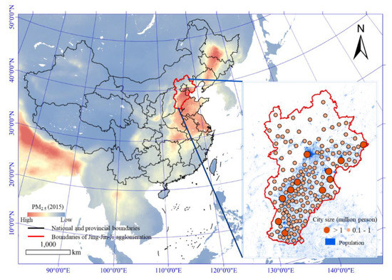
Figure 1.
Geographical location, air pollution level, and population distribution of the study area.
2.2. Schematic Diagram of Concept and Mechanism and the Research Framework
We first drew a schematic diagram of the urban form and impact mechanism (Figure 2a) and outlined the overall research framework to clarify the data processing and modeling process (Figure 2b). In Figure 2a, the diagram first shows the principal indicators of urban form. The AI is calculated from an adjacency matrix and is used as a descriptor of desperation, interspersion, subdivision, or isolation [27]. FRAC values greater than 1 indicate a departure from Euclidean geometry and an increase in shape complexity. This metric can be used across a range of spatial scales and thus overcomes limitations of the straight perimeter/area ratio [28,29,30]. AREA, POPDEN, urban nighttime light (NTL), and nighttime light intensity (NLI) also have close relationships with urban air pollution [31,32]. These indicators of urban form can affect the emission of urban air pollution through the influence on transportation and other paths. They can also affect the diffusion of air pollutants through the impact of urban microclimate and other factors. This brief schematic diagram lays the foundation for our further empirical analysis.
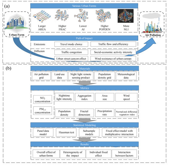
Figure 2.
The schematic diagram of the impact paths of urban form on air pollution (a) and the method flow (b).
As for the method flow (Figure 2b), we first quantified the urban form and air pollution indicators based on multisource data, including land use data, air pollution grid products, night light remote sensing images, POPDEN spatial grids, and meteorological monitored data. Based on these indicators, we built a variety of panel models. We used the Hausman test to determine the appropriate type of panel model, identify individual FEs, and evaluate the overall effect of each factor on air pollution indicators. After that, we built subsample models of all cities according to the natural and social economic conditions of cities, such as elevation and road network density, and we compared the differences of coefficients across models. Finally, we used the FE model with multiple interactions to quantify the interactions between urban form factors. Brief descriptions of some variables involved are listed in Table 1.

Table 1.
Brief description of the variables.
2.3. Data Sources and Metrics
2.3.1. Air Pollution
We used the satellite remote sensing inversion data (annual near-surface PM2.5 and NO2 concentration grids) from 2000, 2005, 2010, and 2015 as the basis to extract air pollution indicators (APIs). This method can overcome the problem of sparse spatial data recorded by air quality monitoring stations and help to obtain long time series and spatially continuous observations. The annual PM2.5 grid data set was derived from a combination of aerosol optical depth (AOD) retrievals from the NASA Moderate Resolution Imaging Spectroradiometer (MODIS), Multiangle Imaging Spectroradiometer (MISR), and Sea-Viewing Wide Field-of-View Sensor (SeaWiFS). The GEOS-Chem chemical transport model and geographically weighted regression model were used to relate the AOD to the near-surface PM2.5 concentration (https://sedac.ciesin.columbia.edu/data/set/sdei-global-annual-gwr-pm2-5-modis-misr-seawifs-aod) [33,34]. The annual ground-level NO2 grids were derived from the Global Ozone Monitoring Experiment (GOME), Scanning Imaging Absorption SpectroMeter for Atmospheric CHartographY (SCIAMACHY), and GOME-2 satellite retrievals. GEOS-Chem (https://sedac.ciesin.columbia.edu/data/set/sdei-global-3-year-running-mean-no2-gome-sciamachy-gome2) was also used to relate the tropospheric NO2 column densities and the NO2 concentrations at ground level [35]. PM2.5 and NO2 grids with original spatial resolutions of 0.01 and 0.1 degrees, respectively, were resampled to 1 km grids for subsequent analysis (Figure 3). Due to the lack of data, we replaced the 2015 NO2 concentration with the 3-year mean of 2010–2012.
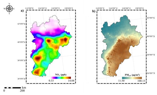
Figure 3.
Spatial pattern of PM2.5 (a) and NO2 (b) concentrations in 2015 for the Beijing-Tianjin-Hebei region.
2.3.2. Urban Form Indicators
We used land use data with a 30 m resolution to extract urban extent and calculate urban geometric indicators. The data were derived from the Resource and Environment Data Cloud Platform, Chinese Academy of Sciences (CAS) (http://www.resdc.cn/DataList.aspx). First, we took 2015 as a reference year for the identification of city samples and their boundaries. We selected the urban patches in 2015 according to the land use classification and merged the connected urban patches into one city sample since some cities may grow beyond their administrative boundaries. In this way, we obtained 150 independent urban units. Then, based upon the boundaries of the 150 urban units and the land use maps in different years, we calculated the landscape metrics AREA, AI, and FRAC for each urban unit in each year. The POPDEN dataset was obtained from the Center for International Earth Science Information Network at Columbia University (available at https://beta.sedac.ciesin.columbia.edu/data/set/gpw-v4-population-count-rev10). The Defense Meteorological Satellite Program (DMSP) Operational Line-scan System (OLS) night time light (NLT) version 4 stable average visible data were obtained from the NOAA, National Geophysical Data Center (http://ngdc.noaa.gov/eog/dmsp/downloadV4composites.html), and then the NTL data were calibrated via the ridgeline sampling regression method to obtain a consistent NLI time series [36]. Due to the lack of NLI data in 2015, we used the data in 2013 as a replacement. The calculations of FRAC and AI were performed in FRAGSTATS 4.2 software developed and supported by Dr. McGarigal and Dr. Cushman.
2.3.3. Control Variables
We further took meteorological and vegetation factors as control variables. The annual average WIND and PREC data were based on the existing Princeton reanalysis data, GLDAS (Global Land Data Assimilation System) data, GEWEX-SRB (Global Energy and Water Cycle Experiment—Surface Radiation Budget) radiation data, and TRMM (Tropical Rainfall Measuring Mission) PREC data as the background field, which are integrated with the records from meteorological stations in China [37]. The meteorological data with a spatial resolution of 0.1 degrees were resampled to 1 km for the zonal statistics. The normalized difference vegetation index (NDVI) was obtained from MODIS datasets (MOD13Q1) with a spatial resolution of 250 m. We used the growing season data as the annual measurement of urban vegetation coverage.
2.4. Statistical Methods
2.4.1. Econometric Models
A panel data model for the period 2000–2015 was utilized in this study. The panel model has several major advantages over conventional cross-sectional or time series models [38,39]: It usually has high-power control of individual heterogeneity and can help reduce the effects of multicollinearity among the variables and increase the degrees of freedom [38]. We used two methods for estimating unobserved effect panel data models, namely, the FE estimator and the random effect estimator. Let APIij be the air pollution indicator of the tth year (t = 2000, 2005, 2010, 2015) in the ith city (I = 1, 2, …, 150). We modeled the relationships between APIs and UFIs:
where APIit is the air pollution indicator of the tth year at the ith urban unit; μ is a scalar coefficient; β is a vector of the parameters; Ui denotes the individual effect of the ith urban unit, capturing the idiosyncratic characteristics of each urban unit; εit denotes the random error of the tth year at the ith urban unit; and UFIit is a vector of the urban form factors.
Before conducting the panel data model, we used the Hausman test to decide whether the FE model or random effect model should be used [40]. We applied the natural logarithm transformation to all the independent variables to avoid nonstationarity and heteroskedasticity phenomena in the time series [41]. A log transformation was applied for APIs, and then the elastic estimation coefficient was obtained.
2.4.2. Subsample Modeling for City in the Context of Various Natural and Social Conditions
To gain insight into the differences in the relationship between urban form and air pollution in the context of various natural and social conditions, we regrouped the cities from three perspectives and modeled them separately. First, we classified the cities according to their built-up areas as of 2015, using the criteria proposed in a previous study [42]. According to urban area size [42,43], these cities were divided into two categories of different sizes, including small-sized cites (≤50 km2) and medium/large-sized cities (>50 km2). Then, we divided all cities into two categories according to their elevation [44], including low-elevation cities (<500 m above sea level) and medium/high-elevation cities (≥500 m). Finally, we calculated the road density based on the road network obtained from the Baidu Map data of 2015, taking into account all levels from national roads to township roads. We divided the cities into low road density cities and high road density cities using the classification criteria determined according to the natural breakpoint of the road density of all cities.
2.4.3. Linear Regression Model with Multiplicative Interaction
Because POPDEN has led to one of the most important debates on compact city issues, we used the linear regression model with multiplicative interaction terms to estimate the conditional marginal effect of POPDEN on air pollution concentrations across different levels of NLI, AI, and FRAC. At the same time, the conditional marginal effect of NLI, AI, or FRAC on air pollution concentrations across different levels of POPDEN were also obtained.
The linear regression model with multiplicative interaction terms is a common model for examining whether the relationship between an outcome Y and a key independent variable D varies with the levels of a moderator X, which is often used to capture the differences in the context [22,45]. For example, the effect of D on Y may grow with higher levels of X. Such conditional hypotheses are ubiquitous in many social and natural sciences, and linear regression models with multiplicative interaction terms are the most widely used framework for testing these conditional hypotheses in applied work [45]. The corresponding formula of this model is as follows:
where APIit is the API of the tth year at the ith urban unit; μ is a scalar coefficient; β is a vector of the parameters; Ui denotes the individual effect of the ith urban unit, capturing the idiosyncratic characteristics of each urban unit; εit denotes the random error of the tth year at the ith urban unit; and UFIit is a vector of the urban form factors. Dit and Xit denote a key independent variable and a moderator variable of the tth year at the ith urban unit, respectively. To verify the robustness of the evaluation of the interaction, we also added the interaction item into the pooled sectional model as a comparison.
Moreover, we used linear interaction diagnostic (LID) plots to illustrate the marginal effect of D on Y. In LID plots, the horizontal axis is X, and the vertical axis is the estimated regression coefficient of D and Y. We further calculated the confidence intervals and binning estimator for comparison and verification, that is, the estimation results based on the regression of subgroups with high (H), medium (M), and low (L) values of the indicators. The graph was drawn using the ‘Interflex’ package of Stata 16 [46].
3. Results
3.1. Change Trends in Air Pollution Level and Urban Form Indicators
From 2000 to 2015, the concentrations of NO2 and PM2.5 in cities showed an upward trend (Figure 4a–c), especially in the central and eastern regions. Urban land expansion was significant, especially from 2010 to 2015, which led to dramatic changes in urban form. The probability density function (PDF) plots (Figure 4d,e) showed that from 2000 to 2015, the average concentrations of NO2 and PM2.5 increased. However, the peak density of NO2 decreased each year, and the density curve became low and fat, indicating that the number of heavily polluted cities increased. The trends in the AI and FRAC were concave curve and convex curve with inflection trends, respectively (Figure 4f). Other indicators of urban morphology, including NLI, AREA, and POPDEN, displayed rising trends. The change in NDVI showed fluctuations. These results showed that the urban form of the Beijing-Tianjin-Hebei urban agglomeration produced an uncertain trend in terms of expansion mode and urban greening, which may be related to the lack of unified macro planning guidance.
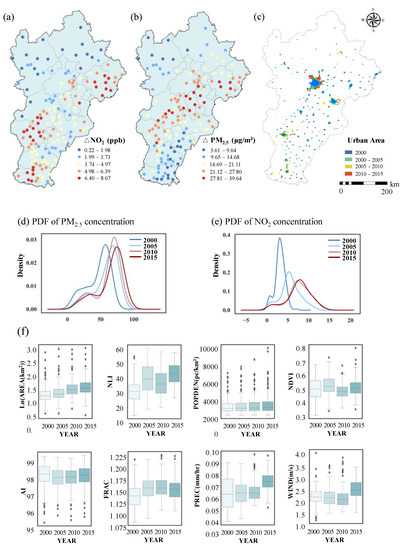
Figure 4.
Changes of PM2.5 (a), NO2 concentration (b), and urban land (c) from 2000 to 2015 and probability density function (PDF) plot of air pollution levels (PM2.5 in (d) and NO2 in (e)). (f) Boxplots of the urban form indicators (UFIs) from 2000 to 2015. The darker color of the boxplot means that the data are more recent. The whiskers encompass 1.5 of the interquartile range (IQR) above the third quartile and below the first quartile.
3.2. Panel Data Model Estimations
The results of the F test and Hausman test showed that it was reasonable to add individual FEs to the panel model (Table 2). The results showed that the combination of AREA, geometry, vegetation, and meteorological factors well fitted the PM2.5 and NO2 concentrations in the individual FE model, and the corresponding R2 values were up to 0.63 and 0.69, respectively (Table 2). The significant estimation coefficients of the influence of all urban morphology indexes on the concentrations of the two pollutants were obtained by FE regression (Table 3). The results showed that the increases in NLI, AREA, POPDEN, AI, and FRAC increased PM2.5 and NO2 concentrations. The increase in WIND significantly reduced the concentrations of the two pollutants. PREC showed a greater effect on PM2.5 concentration but no significant effect on NO2. In contrast, the NDVI showed a greater impact on NO2 than on PM2.5. More significantly, the coefficients (0.1–0.9 for PM2.5 and 0.6–2.2 for NO2) of the three indexes of NLI, AREA, and POPDEN were much lower than those of the two geometric shape indexes (1.8–5.1 for PM2.5 and 5.2–9.7 for NO2), which suggests that the change in AI or FRAC with the same proportion plays a much greater role in air pollution than other UFIs.
Table 2.
Results of the fixed effect (FE) model and individual effect test.
Table 3.
Estimations of the FE models.
3.3. The Relationships between Air Pollution and Urban Form Factors in Cities with Different Conditions
The classification of cities showed that cities below 500 m were mainly located in the North China Plain, while those above 500 m were mainly located in the Bashang Plateau [47] (Figure 5a). Medium and large cities, i.e., cities with an area of more than 50 km2, had relatively scattered geographical distribution (Figure 5b), which was similar to the distribution of cities with higher road network density (Figure 5c). According to the violin charts of PM2.5 and NO2 concentrations in the cities with different scales, elevations and road network densities from 2000 to 2015 (Figure 5d), there were change patterns of the air pollution. The air pollution level in low-elevation and medium/large cities was higher and changed faster. In contrast, cities with sparse road networks had more serious air pollution levels and the most rapidly increased trends.
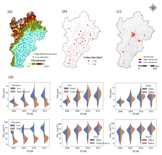
Figure 5.
The locations of cities with different elevations (a), area scales (b), and road network densities (c) and their respective statistical distribution of air pollution levels (d).
The results of sub panel models showed that the coefficients of most factors were similar to the coefficients of the whole regional scale regression (Table A1). However, the effects of various factors on air pollution differed between cities with different elevations, city sizes, and road network densities. In general, the regression R-square of cities with medium/large size, medium/high elevation, and low road network density is higher than that of small cities, cities with low elevation, and high road network density, respectively. As Figure 6 shows, from the perspective of urban scale, in the PM2.5 model, the elasticity coefficients of POPDEN, AI, FRAC, and WIND are significant, and their absolute values are larger in small cities, whereas AREA has a greater impact on air pollution in larger cities. From the perspective of elevation, in the PM2.5 model, POPDEN and PREC have a greater impact on the PM2.5 of the medium/high- elevation cities, while NLI, FRAC, AREA, and WIND have the opposite effect. The difference in the regression coefficient of the NO2 model is consistent with that of the PM2.5 model except for NLI and POPDEN. From the perspective of road network density, NLI and POPDEN have a greater impact on cities with a low road network density, while AREA has a greater impact on cities with a high road network density.
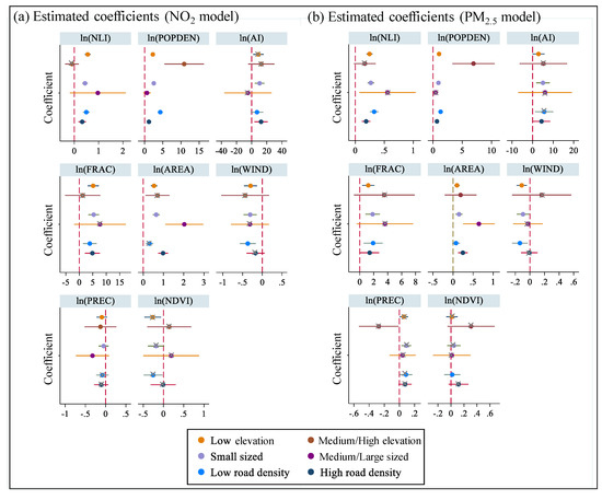
Figure 6.
Estimated coefficients of the FE models of cities with different sizes, elevations, and road densities. Estimated coefficients in NO2 (a) and PM2.5 models (b) and Parameter bounds for the regression slope are the 95% confidence interval. Coefficients with p less than 0.01 are marked with a cross.
3.4. The Internal Interactions of Urban Form Factors
In the FE model and pooled sectional linear model, the multiplicative interaction terms including POPDEN were added, and the regression estimation results are shown in Table 4. In the FE model, only in models A1 and B1, the main effect items and interaction items are statistically significant synchronously, while in the pooled sectional linear model, the interaction items are mostly significant. However, adding the interaction terms of POPDEN and NLI/AI/FRAC significantly increased the R-square of the FE model by approximately 0.06, while the improvement of the pooled sectional model is relatively small or even opposite.
Table 4.
Estimations of the FE panel models with different interaction items.
We focused on the analysis of models A1 and A2 with significant interaction terms and obtained the LID plots shown in Figure 7a–d. As a contrast, we also present the results derived from pooled sectional models, as shown in Figure 7e–h. The results of the binning estimator are also shown on all plots. Figure 7 shows that the positive or negative marginal effects of the binding estimator, the FE model, and the pooled sectional model are consistent, while the binning estimators have wider confidence intervals. There is also clear evidence of an interaction as the slope of the line that captures the relationship between NLI on PM2.5 is positive at low levels of POPDEN, flat at medium levels of POPDEN, and negative at high levels of POPDEN. Figure 7b,d show that when the POPDEN increases, the air pollution in the cities with a low economic development level and low morphological compactness will be impacted more greatly.
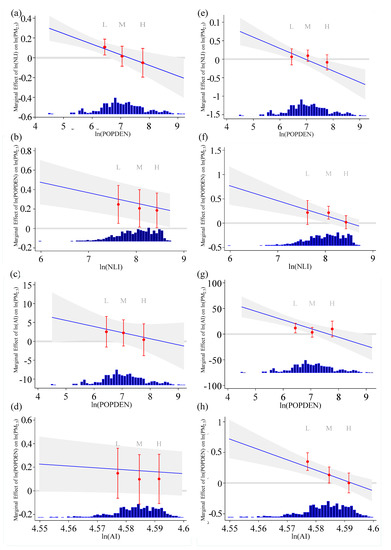
Figure 7.
Linear interaction diagnostic plots. The above plots examine the marginal effects plot, marginal effects estimate from the model (blue line) and the binning estimator (red dots). H, M, and L represent subgroups with high-, medium-, and low-level indicators, respectively. (a–d) illustrate the interactions in the FE model, while (e–h) illustrate the interactions in the pooled sectional model.
4. Discussion
4.1. The Influence of Urban Form on Air Pollution
The rise in AI and FRAC show a negative impact on air quality. Our results regarding AI are consistent with the findings of Yupeng Liu on Chinese cities at the national scale [48,49] and the findings of Qiannan She of the Yangtze River Delta in China [50]. However, these results are inconsistent with the findings of Bereitschaft and Debbage [51] in the United States and the findings of Shi et al. [42] in Chinese cities. Note that the latter used the urban continuity index and percentage of like adjacencies index to represent the urban agglomeration degree. In contrast, our FRAC results are consistent with most of the existing studies [51]. Considering that we set control variables in the regression and used a reliable FE panel model [21], our results provide a reliable reference for understanding the role of urban morphology at the regional scale.
AI represents the dispersion or aggregation distribution of multiple patches, which is closely related to the traffic flow inside and between cities, further affecting the air pollutant emissions caused by traffic [5,52]. On the one hand, the separated leapfrog urban form corresponding to low AI leads to an increase in long-distance travel flow between urban patches, which has been suggested to have a negative impact on urban air quality. On the other hand, the high AI corresponding with an aggregated and monocentric urban form has a negative impact on ventilation and convective efficiency in the city. In addition, the high concentration of corresponding social and economic resources will increase local traffic flow and cause traffic congestion, and the low-efficiency vehicle driving conditions will increase the emissions of NO2 and PM2.5 and accelerate the generation of secondary particles. The negative impact of high AI seems to be more significant in the Beijing-Tianjin-Hebei urban agglomeration than in other regions.
High FRAC can better represent disordered urban sprawl development, and the extra traffic burden it causes can be better correlated with the increase in air pollution emissions. Fragmented cities with highly convoluted, irregular boundaries are expected to have higher nonpoint emissions (primarily from automotive sources) [51], as well as higher secondary aerosol contributions (e.g., NO2 and SO2) to particulate matter (PM) pollution [53]. Although the confirmation of this positive or negative relationship is consistent with the existing research, the relatively larger coefficients of FRAC and AI that we obtained suggest the interesting potential impact of minor changes in urban geometry.
4.2. The Influences of Natural Conditions and Urban Characteristics and Their Implications for Urban Planning
The results of the sub panel models show that planning strategies should be adjusted for cities with different geographical environments and urbanization characteristics. This is consistent with or conflicting with the conclusions of the existing studies based on sub panel or cross-sectional models. For example, for small size cities, the population density and morphological sprawl need to be well managed. This is similar to Bechle et al.’s research results based on 1274 global cities [11], whose study showed that the impact of morphological compactness on the concentration of NO2 in small-population sized cities is significantly higher than that in large-scale cities, and the value of the regression coefficient of the small-scale compactness index is more than twice the value of the global scale regression coefficient. However, our conclusion is inconsistent with that of one research based on 830 cities in East Asia [54]. Larkin et al. found that the impact of urban sprawl index on NO2 concentration is greater in large sized cities, while the impact on PM2.5 concentration is the largest in medium-sized cities. It is worth noting that these two studies used a cross-sectional rather than panel data research design, which might be one important reason for the inconsistent results.
For medium/large cities, it is more important to prevent excessive urban area expansion. This is consistent with the conclusion of another study based on sub panel models, whose results show that urban expansion had more significant positive impacts on PM2.5 concentration in medium/large-sized cites (>50 km2). For the plain cities at low elevation, the control of social economic intensity plays an important role in clean air, but for the cities at medium/high elevation, the control of POPDEN has a profound impact. The influence of elevation on the relationship between urban form and air pollution is closely related to meteorological conditions. The low-elevation areas of the Beijing-Tianjin-Hebei region are mainly located on the North China Plain, which is bordered on the north by the Yanshan Mountains and on the west by the Taihang Mountains’ edge of the Shanxi Plateau [55]. This terrain causes the North China Plain to be dominated by a cold high pressure system with low surface wind speeds, sometimes also accompanied by surface temperature inversion [55]. Therefore, the air pollutants produced by socio-economic activities are favorable for the formation of haze or fog, and usually lead to high levels of pollutants concentration due to weak mixing and dispersion [55,56], and thus the larger regression coefficient corresponding to the variable of NLI. For cities with low road network density, NLI and POPDEN have a greater impact, implying that the improvement of traffic efficiency brought by the construction of adequate traffic infrastructure can effectively reduce the impact of POPDEN and economic growth on air pollution, and possibly a reduction of per capita air pollutant emissions.
4.3. Implications of Interactions among Urban Form Indicators for Urban Planning
In most previous studies, the effect of each urban form indicator was considered separately, without consideration of their interactions. Our research shows that the increase of POPDEN has an overall improvement on the air pollution of the cities in the Beijing-Tian-Hebei region. However, the results of interaction analysis reveal that this effect is context-dependent, which is regulated by social and economic conditions (represented by NLI) and morphological aggregation.
The analysis of the interaction between NLI and POPDEN shows that social and economic development will reduce the impact of population growth density. According to the Environmental Kuznets curve, the development of cities can reduce pollutant emissions through industrial upgrading and the strengthening of clean policies [10,57], which will further restrain the negative impact of POPDEN. Therefore, giving priority to areas with higher economic development levels for the increase of POPDEN, or giving priority to the economic development in areas with more dense populations, may be effective measures to reduce air pollution on the regional scale.
Previous studies suggested that more concentrated cities have great benefits to help control pollutant emissions, heat island effect, carbon emissions, etc. [5,10,41,58]. However, from the perspective of cleaner air, for cities with low population density in the Beijing-Tianjin-Hebei region, the aggregated urban form is not a good choice. What is more informative is that aggregated urban form can inhibit the effect of POPDEN on urban air quality deterioration. That is, more aggregated cities can greatly reduce the negative impact of POPDEN. This is because a more compact city can effectively reduce the average travel distance and travel mode choice of the population on the urban scale, thus affecting the overall pollution emissions. This role can have a greater impact in more densely populated areas. Therefore, in more densely populated areas, it is more urgent to maintain aggregated distribution. At the same time, excessive urban sprawl should be avoided, since it is difficult to reverse urban geometry once it has been built and has a lock-in effect on the city [59,60].
The existence of interactions means that the expansion and development of cities will have a greater joint effect with the evolution of urban forms, which cannot be measured only according to their respective independent functions. The estimated coefficients from traditional linear models should be considered more carefully because interactions will lead to the formation of a complex nonlinear relationship between urban form factors and air pollution indicators and thus not be robust.
5. Conclusions
In this paper, we studied the role of urban form in air pollution based on a panel data model from multiple perspectives, including elevation, area size, and road density. The results show that the expansion of AREA, the increase in NLI, high POPDEN, an aggregated layout, and a disordered sprawl aggravate air pollution. Among the urban form factors, the elastic coefficients of the urban AI and FRAC are highest at the regional scale. However, NLI, POPDEN, AI, and FRAC are all more influential in small cities, while AREA has the opposite trend. POPDEN has a greater impact on medium/high-elevation cities, while NLI and FRAC have a greater impact on low-elevation cities. NLI and POPDEN have a greater impact on low-density road network cities, while AREA does not.
The result of the linear regression model with multiplicative interaction provides evidence of interactions between POPDEN and NLI or AI as the slope of the line that captures the relationship between NLI on PM2.5 is positive at low levels of POPDEN, flat at medium levels of POPDEN, and negative at high levels of POPDEN. When the POPDEN increases, the air pollution in a city with low economic development level and low aggregation degree will be impacted more greatly. The results imply that in the process of urban development or expansion, urban form optimization and context-dependent adjustment are urgent.
The first limitation of our study is that most of the urban samples used were small and medium-sized cities, and more samples are needed to confirm the patterns in medium/large cities. Second, the relationship between urban form and air pollution may change with season [49], but we did not consider seasonal variations. Third, this work focused on the regional scale. Although more accurate assessment can be obtained for these cities, larger-scale observations are necessary because of the strong heterogeneity of the background characteristics of global cities. Finally, our linear regression model with multiplicative interaction maintained an important assumption: that the interaction effect is linear. The linear interaction effect assumption often fails in empirical settings because many interaction effects are not linear, and some may not even be monotonic. In future studies, it will be meaningful if the complex interaction among more variables can be included based on a machine learning algorithm (such as random forest, Gradient Boosting model, or corresponding multi-objective learning model), which will further deepen the insight into the impact of multi-perspective urban form on air pollution.
Author Contributions
Conceptualization, Z.L.; Formal analysis, F.W. and Y.W.; Funding acquisition, S.L.; Investigation, F.W., Y.W., H.J., and F.S.; Methodology, Z.L.; Resources, Y.W. and H.J.; Supervision, S.L.; Writing—original draft, Z.L.; Writing—review and editing, J.H. All authors have read and agreed to the published version of the manuscript.
Funding
This research was funded by the Major Projects of the National Natural Science Foundation of China, grant number 41590843.
Acknowledgments
We thank the Major Projects of the National Natural Science Foundation of China (grant number 41590843) for its support. We are also grateful to the editor and the reviewers for their helpful comments.
Conflicts of Interest
No conflict of interest exits in the submission of this manuscript, and it has been approved by all authors for publication. The work described was original research that has not been published previously and is not under consideration for publication elsewhere, in whole or in part. All of the authors listed have approved the manuscript that is enclosed.
Appendix A
Table A1.
Estimations of the FE models of different sizes, elevations, and road densities.
Table A1.
Estimations of the FE models of different sizes, elevations, and road densities.
| Model of PM2.5 | Model of NO2 | |||||||||||
|---|---|---|---|---|---|---|---|---|---|---|---|---|
| Area Size | Elevation | Road Density | Area Size | Elevation | Road Density | |||||||
| Small | Medium/Large | Low | Medium/High | Low | High | Small | Medium/Large | Low | Medium/High | Low | High | |
| ln(NLI) | 0.268 *** | 0.556 * | 0.245 *** | 0.165 | 0.325 *** | 0.187 *** | 0.440 *** | 0.968 | 0.551 *** | −0.0936 | 0.496 *** | 0.326 *** |
| (9.47) | (2.36) | (9.56) | (1.76) | (8.63) | (4.95) | (8.03) | (1.73) | (9.23) | (-0.67) | (6.99) | (4.26) | |
| ln(POPDEN) | 0.932 *** | 0.451 * | 1.032 *** | 6.921 *** | 1.301 *** | 0.673 *** | 2.522 *** | 0.651 | 2.260 *** | 10.90 *** | 4.306 *** | 1.186 *** |
| (7.58) | (2.14) | (10.98) | (3.83) | (6.76) | (5.29) | (10.58) | (1.30) | (10.32) | (4.02) | (11.90) | (4.60) | |
| ln(AI) | 5.031 ** | 6.050 | 2.872 | 5.243 | 5.643 * | 4.344 * | 10.56 ** | −4.887 | 8.875 * | 12.72 | 7.047 | 12.41 ** |
| (3.03) | (0.95) | (1.93) | (0.91) | (2.53) | (2.01) | (3.27) | (−0.32) | (2.56) | (1.47) | (1.68) | (2.83) | |
| ln(FRAC) | 1.842 *** | 3.607 | 1.222 ** | 3.511 | 1.914 ** | 1.419 * | 5.352 *** | 7.690 | 5.151 *** | 1.264 | 3.906 ** | 4.869 *** |
| (3.51) | (1.84) | (2.73) | (1.62) | (2.77) | (2.06) | (5.25) | (1.65) | (4.94) | (0.39) | (3.01) | (3.48) | |
| ln(AREA) | 0.149 *** | 0.644 ** | 0.0981 ** | 0.188 | 0.0740 | 0.245 *** | 0.642 *** | 2.031 *** | 0.533 *** | 0.705 * | 0.310 *** | 0.981 *** |
| (3.43) | (3.37) | (2.91) | (0.95) | (1.52) | (4.09) | (7.61) | (4.47) | (6.78) | (2.38) | (3.39) | (8.05) | |
| ln(WIND) | −0.0943 * | −0.0271 | −0.112 ** | 0.162 | −0.137 * | −0.00764 | −0.308 *** | −0.313 | −0.298 *** | −0.433 | −0.368 *** | −0.170 |
| (−2.16) | (−0.28) | (−3.10) | (0.80) | (−2.50) | (-0.13) | (−3.64) | (−1.34) | (-3.54) | (-1.43) | (−3.59) | (−1.47) | |
| ln(PREC) | 0.0915 ** | 0.0421 | 0.0588 * | −0.272 * | 0.0868 * | 0.0758 | −0.0501 | −0.324 | −0.0942 | −0.127 | −0.0802 | −0.109 |
| (2.81) | (0.50) | (2.07) | (−2.09) | (2.09) | (1.74) | (−0.79) | (−1.63) | (−1.42) | (−0.65) | (−1.03) | (−1.23) | |
| ln(NDVI) | 0.0450 | 0.0124 | 0.0151 | 0.310 | 0.0196 | 0.117 | −0.184 | 0.192 | −0.266 * | 0.142 | −0.255 * | −0.00773 |
| (0.85) | (0.09) | (0.34) | (1.71) | (0.31) | (1.51) | (−1.79) | (0.58) | (−2.54) | (0.52) | (−2.16) | (−0.05) | |
| Cons. | −28.18 *** | −33.87 | −18.58 ** | −71.02 * | −33.81 ** | −23.50 * | −67.62 *** | 3.172 | −58.63 *** | −129.3 ** | −63.67 ** | −68.26 *** |
| (−3.72) | (−1.19) | (−2.76) | (−2.41) | (−3.31) | (−2.40) | (−4.60) | (0.05) | (−3.73) | (−2.93) | (−3.31) | (−3.44) | |
| N | 546 | 54 | 516 | 84 | 328 | 272 | 546 | 54 | 516 | 84 | 328 | 272 |
| R2 | 0.623 | 0.854 | 0.660 | 0.783 | 0.654 | 0.647 | 0.714 | 0.831 | 0.709 | 0.753 | 0.751 | 0.713 |
Note: In parentheses are the t statistics corresponding to the coefficients. The t statistics in parentheses = “* p < 0.05, ** p < 0.01, *** p < 0.001”.
References
- Friedrich, M. WHO’s Top Health Threats for 2019. JAMA 2019, 321, 1041. [Google Scholar] [CrossRef] [PubMed]
- Nations, U. 2018 Revision of World Urbanization Prospects; United Nations: New York, NY, USA, 2018. [Google Scholar]
- Breiman, L. Random Forests. Mach. Learn. 2001, 45, 5–32. [Google Scholar] [CrossRef]
- Marquez, L.; Smith, N.C. A framework for linking urban form and air quality. Environ. Model. Softw. 1999, 14, 541–548. [Google Scholar] [CrossRef]
- Rodríguez, M.C.; Dupont-Courtade, L.; Oueslati, W. Air pollution and urban structure linkages: Evidence from European cities. Renew. Sustain. Energy Rev. 2016, 53, 1–9. [Google Scholar]
- Stone, B., Jr. Urban sprawl and air quality in large US cities. J. Environ. Manag. 2008, 86, 688–698. [Google Scholar] [CrossRef]
- Ahlfeldt, G.; Pietrostefani, E. The Effects of Compact Urban Form: A Qualitative and Quantitative Evidence Review; The Coalition for Urban Transitions: Washington, DC, USA; London, UK, 2017. [Google Scholar]
- Mccarty, J.; Kaza, N. Urban form and air quality in the United States. Landsc. Urban Plan. 2015, 139, 168–179. [Google Scholar] [CrossRef]
- Clark, L.P.; Millet, D.B.; Marshall, J.D. Air quality and urban form in US urban areas: Evidence from regulatory monitors. Environ. Sci. Technol. 2011, 45, 7028–7035. [Google Scholar] [CrossRef]
- Bechle, M.J.; Millet, D.B.; Marshall, J.D. Effects of income and urban form on urban NO2: Global evidence from satellites. Environ. Sci. Technol. 2011, 45, 4914–4919. [Google Scholar] [CrossRef]
- Bechle, M.J.; Millet, D.B.; Marshall, J.D. Does urban form affect urban NO2? Satellite-based evidence for more than 1200 cities. Environ. Sci. Technol. 2017, 51, 12707–12716. [Google Scholar] [CrossRef]
- Yuan, M.; Song, Y.; Huang, Y.; Hong, S.; Huang, L. Exploring the association between urban form and air quality in China. J. Plan. Educ. Res. 2017, 38, 413–426. [Google Scholar] [CrossRef]
- Burton, E. The compact city: Just or just compact? A preliminary analysis. Urban Stud. 2000, 37, 1969–2006. [Google Scholar] [CrossRef]
- Neuman, M. The compact city fallacy. J. Plan. Educ. Res. 2005, 25, 11–26. [Google Scholar] [CrossRef]
- Bennett, M.; Saab, A. Modelling of the urban heat island and of its interaction with pollutant dispersal. Atmos. Environ. 1982, 16, 1797–1822. [Google Scholar] [CrossRef]
- Eliasson, I.; Holmer, B. Urban Heat Island Circulation in Göteborg, Sweden. Theor. Appl. Clim. 1990, 42, 187–196. [Google Scholar] [CrossRef]
- Vukovich, F.M.; King, W.J.; Dunn, J.W.; Word, J.J.B. Observations and Simulations of the Diurnal Variation of the Urban Heat Island Circulation and Associated Variations of the Ozone Distribution: A Case Study. J. Appl. Meteorol. 2010, 18, 836–854. [Google Scholar] [CrossRef]
- Cairnes and Lorraine. The Compact City: A Sustainable Urban Form. Urban Des. Int. 1996, 1, 293–294. [Google Scholar] [CrossRef]
- Rydin, Y. Environmental dimensions of residential development and the implications for local planning practice. J. Environ. Plan. Manag. 1992, 35, 43–61. [Google Scholar] [CrossRef]
- Zhou, B.; Rybski, D.; Kropp, J.P. The role of city size and urban form in the surface urban heat island. Sci. Rep. 2017, 7, 4791. [Google Scholar] [CrossRef]
- Wooldridge, J. Introductory Econometrics: A Modern Approach; Thomson/South-Western: Mason, OH, USA, 2006. [Google Scholar]
- Brambor, T.; Clark, W.R.; Golder, M. Understanding interaction models: Improving empirical analyses. Political Anal. 2006, 14, 63–82. [Google Scholar] [CrossRef]
- Braumoeller, B.F. Hypothesis testing and multiplicative interaction terms. Int. Organ. 2004, 58, 807–820. [Google Scholar] [CrossRef]
- Zhang, Z.; Wang, W.; Cheng, M.; Liu, S.; Xu, J.; He, Y.; Meng, F. The contribution of residential coal combustion to PM2.5 pollution over China’s Beijing-Tianjin-Hebei region in winter. Atmos. Environ. 2017, 159, 147–161. [Google Scholar] [CrossRef]
- Zhu, L.; Gan, Q.; Liu, Y.; Yan, Z. The impact of foreign direct investment on SO2 emissions in the Beijing-Tianjin-Hebei region: A spatial econometric analysis. J. Clean. Prod. 2017, 166, 189–196. [Google Scholar] [CrossRef]
- Gong, Y.; Li, J.; Li, Y. Spatiotemporal characteristics and driving mechanisms of arable land in the Beijing-Tianjin-Hebei region during 1990–2015. Socio-Econ. Plan. Sci. 2019, 100720. [Google Scholar] [CrossRef]
- He, H.S.; Dezonia, B.E.; Mladenoff, D.J. An aggregation index (AI) to quantify spatial patterns of landscapes. Landsc. Ecol. 2000, 15, 591–601. [Google Scholar] [CrossRef]
- Mandelbrot, B.B. Fractals: Form, Chance and Dimension; Mandelbrot, B.B., Ed.; WH Freeman & Co.: San Francisco, CA, USA, 1979. [Google Scholar]
- Mandelbrot, B.B. The Fractal Geometry of Nature; WH Freeman: New York, NY, USA, 1983; Volume 173. [Google Scholar]
- Milne, B.T. Lessons from applying fractal models to landscape patterns. Ecol. Stud. 1991, 82, 199–235. [Google Scholar]
- Gao, B.; Huang, Q.; He, C.; Ma, Q. Dynamics of urbanization levels in China from 1992 to 2012: Perspective from DMSP/OLS nighttime light data. Remote Sens. 2015, 7, 1721–1735. [Google Scholar] [CrossRef]
- Ma, T.; Zhou, Y.; Zhou, C.; Haynie, S.; Pei, T.; Xu, T. Night-time light derived estimation of spatio-temporal characteristics of urbanization dynamics using DMSP/OLS satellite data. Remote Sens. Environ. 2015, 158, 453–464. [Google Scholar] [CrossRef]
- Van Donkelaar, A.; Martin, R.V.; Brauer, M.; Hsu, N.C.; Kahn, R.A.; Levy, R.C.; Lyapustin, A.; Sayer, A.M.; Winker, D.M. Global Annual PM2.5 Grids from MODIS, MISR and SeaWiFS Aerosol Optical Depth (AOD) with GWR, 1998–2016; NASA Socioeconomic Data and Applications Center (SEDAC): New York, NY, USA, 2018.
- Van Donkelaar, A.; Martin, R.V.; Brauer, M.; Hsu, N.C.; Kahn, R.A.; LevyiD, R.; Lyapustin, A.; Sayer, A.M.; Winker, D. Global Estimates of Fine Particulate Matter using a Combined Geophysical-Statistical Method with Information from Satellites, Models, and Monitors. Environ. Sci. Technol. 2016, 50, 3762–3772. [Google Scholar] [CrossRef]
- Geddes, J.; Martin, R.V.; Boys, B.L.; Van Donkelaar, A. Long-term trends worldwide in ambient NO2 concentrations inferred from satellite observations. Environ. Health Perspect. 2016, 124, 281–289. [Google Scholar] [CrossRef]
- Zhang, Q.; Pandey, B.; Seto, K.C. A Robust Method to Generate a Consistent Time Series from DMSP/OLS Nighttime Light Data. IEEE Trans. Geosci. Remote Sens. 2016, 54, 5821–5831. [Google Scholar] [CrossRef]
- Chen, Y.; Yang, K.; He, J.; Qin, J.; Shi, J.; Du, J.; He, Q. Improving land surface temperature modeling for dry land of China. J. Geophys. Res. Space Phys. 2011, 116, D20104. [Google Scholar] [CrossRef]
- Al-mulali, U. Factors affecting CO2 emission in the Middle East: A panel data analysis. Energy 2012, 44, 564–569. [Google Scholar] [CrossRef]
- Du, L.; Wei, C.; Cai, S. Economic development and carbon dioxide emissions in China: Provincial panel data analysis. China Econ. Rev. 2012, 23, 371–384. [Google Scholar] [CrossRef]
- Hausman, J.A. Specification Tests in Econometrics. Econometrica 1978, 46, 1251–1271. [Google Scholar] [CrossRef]
- Fang, C.; Wang, S.; Li, G. Changing urban forms and carbon dioxide emissions in China: A case study of 30 provincial capital cities. Appl. Energy 2015, 158, 519–531. [Google Scholar] [CrossRef]
- Shi, K.; Wang, H.; Yang, Q.; Wang, L.; Sun, X.; Li, Y. Exploring the relationships between urban forms and fine particulate (PM2.5) concentration in China: A multi-perspective study. J. Clean. Prod. 2019, 231, 990–1004. [Google Scholar] [CrossRef]
- Chen, Q.; Cai, B.; Dhakal, S.; Pei, S.; Liu, C.; Shi, X.; Hu, F. CO2 emission data for Chinese cities. Resour. Conserv. Recycl. 2017, 126, 198–208. [Google Scholar] [CrossRef]
- Giussani, D.A.; Phillips, P.S.; Anstee, S.; Barker, D.J.P. Effects of Altitude versus Economic Status on Birth Weight and Body Shape at Birth. Pediatr. Res. 2001, 49, 490–494. [Google Scholar] [CrossRef]
- Hainmueller, J.; Mummolo, J.; Xu, Y. How Much Should We Trust Estimates from Multiplicative Interaction Models? Simple Tools to Improve Empirical Practice. Political Anal. 2019, 27, 163–192. [Google Scholar] [CrossRef]
- Xu, Y.; Hainmueller, J.; Mummolo, J.; Liu, L. INTERFLEX: Stata Module to Estimate Multiplicative Interaction Models with Diagnostics and Visualization; Statistical Software Components: Boston, MA, USA, 2017. [Google Scholar]
- Zhai, Q.; Guo, Z.; Li, Y.; Li, R. Annually laminated lake sediments and environmental changes in Bashang Plateau, North China. Palaeogeogr. Palaeoclimatol. Palaeoecol. 2006, 241, 95–102. [Google Scholar] [CrossRef]
- Liu, Y.; Wu, J.; Yu, D. Disentangling the complex effects of socioeconomic, climatic, and urban form factors on air pollution: A case study of China. Sustainability 2018, 10, 776. [Google Scholar] [CrossRef]
- Liu, Y.; Wu, J.; Yu, D.; Ma, Q. The relationship between urban form and air pollution depends on seasonality and city size. Environ. Sci. Pollut. Res. 2018, 25, 15554–15567. [Google Scholar] [CrossRef] [PubMed]
- She, Q.; Peng, X.; Xu, Q.; Long, L.; Wei, N.; Liu, M.; Jia, W.; Zhou, T.; Han, J.; Xiang, W. Air quality and its response to satellite-derived urban form in the Yangtze River Delta, China. Ecol. Indic. 2017, 75, 297–306. [Google Scholar] [CrossRef]
- Bereitschaft, B.; Debbage, K. Urban form, air pollution, and CO2 emissions in large US metropolitan areas. Prof. Geogr. 2013, 65, 612–635. [Google Scholar] [CrossRef]
- Zhang, N.; Huang, H.; Duan, X.; Zhao, J.; Su, B. Quantitative association analysis between PM2.5 concentration and factors on industry, energy, agriculture, and transportation. Sci. Rep. 2018, 8, 1–9. [Google Scholar] [CrossRef]
- Huang, R.-J.; Zhang, Y.; Bozzetti, C.; Ho, K.-F.; Cao, J.; Han, Y.; Daellenbach, K.R.; Slowik, J.G.; Platt, S.; Canonaco, F.; et al. High secondary aerosol contribution to particulate pollution during haze events in China. Nature 2014, 514, 218–222. [Google Scholar] [CrossRef]
- Larkin, A.; Van Donkelaar, A.; Geddes, J.; Martin, R.V.; Hystad, P. Relationships between changes in urban characteristics and air quality in East Asia from 2000 to 2010. Environ. Sci. Technol. 2016, 50, 9142–9149. [Google Scholar] [CrossRef]
- Zhao, X.; Zhao, P.S.; Xu, J.; Meng, W.; Pu, W.W.; Dong, F.; He, D.; Shi, Q.F. Analysis of a winter regional haze event and its formation mechanism in the North China Plain. Atmos. Chem. Phys. 2013, 13, 5685–5696. [Google Scholar] [CrossRef]
- Xu, W.Y.; Zhao, C.S.; Ran, L.; Deng, Z.Z.; Liu, P.F.; Ma, N.; Lin, W.L.; Xu, X.B.; Yan, P.; He, X.; et al. Characteristics of pollutants and their correlation to meteorological conditions at a suburban site in the North China Plain. Atmos. Chem. Phys. 2011, 11, 4353–4369. [Google Scholar] [CrossRef]
- Azam, M.; Khan, A.Q. Testing the Environmental Kuznets Curve hypothesis: A comparative empirical study for low, lower middle, upper middle and high income countries. Renew. Sustain. Energy Rev. 2016, 63, 556–567. [Google Scholar] [CrossRef]
- Liang, Z.; Wu, S.; Wang, Y.; Wei, F.; Huang, J.; Shen, J.; Li, S. The relationship between urban form and heat island intensity along the urban development gradients. Sci. Total. Environ. 2020, 708, 135011. [Google Scholar] [CrossRef] [PubMed]
- Avner, P.; Rentschler, J.; Hallegatte, S. Carbon Price Efficiency: Lock-in and Path Dependence in Urban Forms and Transport Infrastructure; No.6941; The World Bank: Washington, DC, USA, 2014. [Google Scholar]
- Ürge-Vorsatz, D.; Rosenzweig, C.; Dawson, R.; Rodriguez, R.S.; Bai, X.; Barau, A.S.; Seto, K.C.; Dhakal, S. Locking in positive climate responses in cities. Nat. Clim. Chang. 2018, 8, 174–177. [Google Scholar] [CrossRef]


© 2020 by the authors. Licensee MDPI, Basel, Switzerland. This article is an open access article distributed under the terms and conditions of the Creative Commons Attribution (CC BY) license (http://creativecommons.org/licenses/by/4.0/).