Refining Urban Built-Up Area via Multi-Source Data Fusion for the Analysis of Dongting Lake Eco-Economic Zone Spatiotemporal Expansion

Abstract

Rapid urbanization has given rise to serious urban problems. It is crucial to understand the urbanization process to accurately and quickly identify boundary changes in urban built-up areas and implement planning schemes and adjustments in scientific and effective ways. This study proposes a new method to automate and refine the extraction of urban built-up areas by using Landsat and nighttime light (NTL) imagery. The urban agglomeration of Dongting Lake Ecological Economic Zone (UADLEEZ) Landsat data are mapped to NTL data using resampling, superpixel segmentation, and assigning the blank part with the Euclidean distance method. We then compared our findings with those produced via traditional threshold extraction methods. In total, 33 built-up areas of UADLEEZ boundary maps were produced between 1992 and 2018. Thus, we reached the following conclusions: (1) the urban built-up areas obtained via our proposed method are finer than those obtained via other threshold extraction methods; (2) we applied the extraction method to UADLEEZ, and analyzed the expansion of the urban agglomeration based on expansion scale, gravity center offset, and landscape pattern index, the analysis of expansion process is consistent with the actual situation; (3) the proposed method can be used to draw long-term dynamic maps of urban extents in units of years, and the results can be used to update the existing products. This study can serve as a reference for future urban planning, and provide both adjustment programs for relevant departments, and an objective basis for governmental decision-making.

1. Introduction

In recent years, rapid population, economic, and social development have accelerated urbanization processes in China, leading to a sharp expansion in urban construction land [1]. The urban built-up area in China expanded from 17,416 km² in 1992 to 58,456 km² in 2018, and the urbanization rate increased from 27.63% to 59.58% during that same period. Because of the increasing pressure resulting from urban land expansion, mapping urban boundaries at regional or larger scales has become an urgent task. Driven by the urbanization process and economic development, urban areas continue to spread to the hinterland of rural areas, the loss of agricultural land has threatened and damaged the ecological environment, and caused a series of social problems, including insufficient resources, land growth rate being higher than population growth rate, and economic problems. Understanding urbanization processes is therefore crucial and doing so requires a more effective scientific method to extract data regarding urban built-up areas. However, mapping built-up areas involves significant challenges due to the high spatial frequency and heterogeneity of surface features [2].

Since the 1970s, remote sensing (RS) data have been collected using various sensors and recorded at multifarious resolutions, including spectral and temporal resolutions. The revolution in these data has transformed the scale and methods of urban research. As modified satellite imagery has become conveniently available, urban expansion surveillance capacities have been enhanced, especially when it comes to monitoring the spatio-temporal expansion of new urban built-up areas [3]. However, in previous studies, most of these maps are only available for one or two years [4,5]. The ability to understand urbanization processes has been limited at the geographic scale due to the lack of ground-referenced data and extensive satellite data, as well as computational deficiencies. Global Human Settlement Layer (GHSL) is frequently used in the global understanding of urbanization trends and dynamics. It provides us with a systematic differentiation and identification method of built-up area and non-built-up area, which can draw large-scale and complex human settlement information map with unprecedented spatial resolution and spatial scale. Covers a fairly long time series (1975, 1990, 2000, and 2014). GHSL has advantages in studying urbanization process and human settlement environment, but obtaining a fresh picture of urban built-up areas over continuous long periods of time is difficult [6,7]. NTL data (DMSP/OLS and NPP-VIIRS) are associated with developed urban construction land [8,9,10], can be used to deduce socio-economic activities at the city or regional levels [11,12], and to predict the extension of urban built-up areas [13,14]. NTL data have been used alone in the new cluster-based methods; because of their high sensitivity to light, they are used to obtain global land areas [15], but these data contain lights from roads, ports, and industrial fields, which reduce accuracy, and the supporting data are limited, meaning they cannot be analyzed for longer periods [16]. Landsat data have been widely used in urban expansion analyses [17,18], and are ideal data references for drawing land cover maps [19]. Liu et al. used the Landsat imagery to map the expansion of the middle Yangtze River basin [20]. However, problems remain in data research, including the huge data processing workload, and the large spectral differences between ground features, which hinders the automation of urban boundary extraction at national or large regional scales [21,22]. Both kinds of data have their advantages and disadvantages. A single NTL dataset suffers from the blooming effect problem, which can be alleviated via the integration of Landsat data [23,24]. Combining the advantages of these two types of data, we extracted the built-up area of the urban agglomeration (UA) and studied how it expanded and changed.

Many scholars have also attempted to combine the characteristics of NTL and Landsat data from multiple sources to draw urban built-up area maps. The approaches can generally be divided into two categories: the supervised and unsupervised classification, and the automated and semi-automated classification [25,26]. The current methods for extracting urban built-up areas include the deep learning method [27], the index method [28], the cluster-based method [15], and the threshold segmentation method [29], etc. These approaches are designed to transform data into meaningful information about human activities and changes in urban built-up areas. Han et al. used deep learning methods to classify Landsat imagery and analyzed changes in urban expansion. The overall accuracy and Kappa coefficient of deep learning are high, and the rate of misjudgment is low. However, due to the complexity of the graph model in deep learning, the time complexity of the algorithm has increased dramatically, and a large amount of data are required to support it [27]. Wu et al. used DMSP/OLS data and Landsat-7 data to extract the urban built-up areas via the weighted fusion method. This integrated approach to urban built-up areas is more reliable. However, the study also had many problems including the fuzzy definition of urban built-up areas, the lack of ground truth value, and the fact that it did not put forward a method for verifying the accuracy of the results [30]. Ke et al. proposed an unsupervised urban region extraction method combining Landsat data with DMSP/OLS data, which can reliably and efficiently extract large-scale urban areas; however, in the case of a single city, the results produced by this method for economically developed cities (such as Shanghai) are not ideal [31]. Roychowdhury et al. separately classified the land cover types of Landsat data, divided the luminance region of DMSP data, and used the optimal threshold method to classify urban and non-urban regions. The accuracy of their classifications of urban, suburban and rural land cover types were all above 90%. However, the authors did not combine the advantages of these two types of data, where scaling may lead to threshold errors, and thus could not avoid the blooming effect [32]. Tang et al. combined Landsat-8 data with NPP-VIIRS data to extract and analyze urban construction land. They constructed a new calculation method that effectively eliminated low-density vegetation and bare land information from the results. However, due to the large differences in resolution between the two types of data, some information was missing, and they were unable to eliminate mining areas and large construction fields in the region [33]. The above examples demonstrate that current methods are unlikely to improve the credibility and effectiveness of the extraction of urban built-up areas, and to solve related problems of quantify urban expansion.

In the process of extracting UA built-up areas, determining how to design or learn better methods to retain and characterize details, and how to select the most suitable strategy is of primary importance. We considered combining the advantages of NTL and Landsat data to optimize data noise and avoid errors and omissions in information acquisition. This approach can be applied to different types of land cover, and used to conduct research in larger areas and continuously monitor for longer periods. Crucially, it does not rely on expensive manual tagging examples and adjustments to local parameters. It can quickly and accurately extract information about UA built-up areas, and is highly accurate compared to other available methods [34,35,36,37].

To better solve the above problems, we developed a new method that combined the advantages of NTL and Landsat data, which we called the superpixel segmentation with assignment method (SSAM). Figure 1 illustrates this process in detail. In this way, we extracted the information of UADLEEZ urban built-up area and examined the spatiotemporal expansion from 1992 to 2018. Following this, we quantitatively analyzed the process of extension through expansion scale, gravity center offset, and landscape pattern index. It provides a valuable model for the extraction and mapping of urban built-up areas as well as for research regarding and engagement in urban, regional, and global human activities [38,39,40].

2. Study Areas and Data Sources

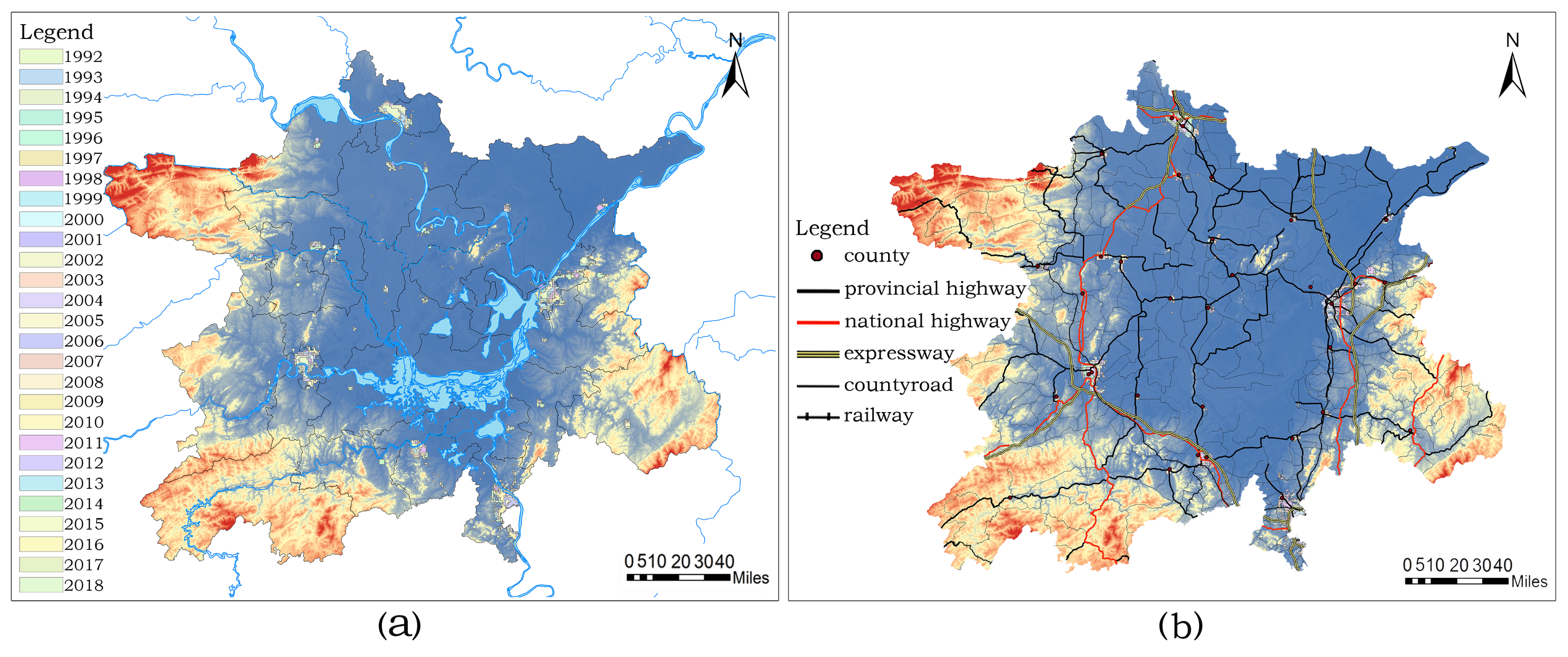
2.1. Study Areas

The study area for this research was the UADLEEZ (as shown in Figure 2), an important water storage lake and international wetland in the middle reaches of the Yangtze River. It spans two provinces, Hunan and Hubei, and has the unique advantages of connecting the east to the west and the south to the north. In accordance with the principles of “ecological priority, comprehensive management, cluster development, and win-win cooperation”, a “one circle, four belts, and four groups” space development pattern will be created. As of 2018, the planned area was 60,500 km² with a permanent population of about 23.38 million and a regional GDP of about $153.46 billion. Promoting the establishment of a “beautiful and rich Great Lakes Economic Zone” is a major measure of a broader strategy designed to bolster the rise of the central region. Exploring the Great Lakes region, guiding the new path of economic and social development with ecological civilization construction, promoting the integrated development of the middle reaches of the Yangtze River, and the opening up development of the Yangtze River Basin are crucial goals. Therefore, we believe that our selection of UADLEEZ as the research area for this study was scientific and representative.

In 2014, the State Council approved the “Dongting Lake Ecological Economic Zone Plan” and defined its regional scope. The UADLEEZ encompasses 33 counties (four cities and one district) including Jingzhou City in Hubei Province and Yiyang City, Changde City, Yueyang City, and the Wangcheng District of Changsha City in Hunan Province.

Table 1. Research area of the urban agglomeration of Dongting Lake Ecological Economic Zone (UADLEEZ).

Province	City	District	County-Level City	County
Hubei	Jingzhou	Shashi,	Songzi,	Jiangling,
		Jingzhou	Shishou, Honghu	Gong’an, Jianli
Hunan	Yiyang	Ziyang,	Yuanjiang	Anhua,
		Heshan		Taojiang, Nan
	Changde	Wuling,	Jin	Hanshou, Taoyuan,
		Dingcheng		Linyi, Shimen, Li, Anxiang
	Yueyang	Yueyang Tower,	Miluo,	Yueyang, Pingjiang,
		Junshan, Yunxi	Linxiang	Xiangyin, Huarong
	Changsha	Wangcheng

includes related details.

2.2. Data Sources

RS has been recognized as an important source of continuous and consistent data, and has been used to study urbanization and related changes on various spatial and temporal scales. In this study, we mainly combined NTL with Landsat RS data, as well as a small amount of statistical yearbook data and actual reference data for analysis.

2.2.1. NTL Data

DMSP/OLS RS data from the Earth Observation Group (EOG) (https://www.ngdc.noaa.gov/eog/dmsp/); since September 1976, the first US Defense Meteorological Satellite Program (DMSP) satellite OLS sensors were used to start acquiring data. The digital information obtained after 1992 provides a new form of research data on large-scale urban expansion. In this study, we extracted DMSP/OLS data from 1992 to 2013. These data eliminate the effects of unexpected light, such as clouds, smoke, and flares. They directly average the gray values from visible detection throughout the year, and are used for grid gray RS. The image gray value range is 0–63, where 63 represents the saturated gray value.

NPP-VIIRS RS data from the EOG (https://ngdc.noaa.gov/eog/viirs/); the first launch of the US New Generation National Polar Orbiting Business Environment Satellite System Suomi-NPP satellite in October 2011. In this study, we extracted the Tile_3 (75N/060E) VIIRS/DNB data from 2014 to 2018 and combined the monthly VIIRS data to obtain the annual average. This data eliminates moonlight illumination under the micro-light channel, and the accuracy of radiation resolution correction is high. As the gray level increases, the pixels do not have saturation values, the spatial resolution increases, and the pixel jump decreases.

While existing urban research has used DMSP/OLS data extensively, relatively few studies have examined and applied NPP-VIIRS data. NTL data differ from traditional statistical data, offering more uniform indicators for spacious urban mapping and reduce regional differences [41]. In urban studies, combining DMSP/OLS with NPP-VIIRS has great advantages, including maintaining the continuity of temporal sequences [42].

2.2.2. Landsat Data

NASA and USGS jointly manage Landsat series satellites to monitor global resources and the environment. They have high spatial resolution (30 m) and large spatial coverage, and provide rich spectral and spatial information. Suitable for extraction and expansion analysis of single cities or regional areas, data can be derived from the Geospatial Data Cloud website (http://www.gscloud.cn/) and USGS (https://www.usgs.gov/). More than 240 Landsat images extracted in this paper, to choose good quality data, we used Landsat-5 data (1992–2000, 2003, 2006 and 2008–2010), Landsat-7 data (2001, 2002, 2004, 2005, 2007, 2011, and 2012), and Landsat-8 data (2013–2018).

Landsat data have the advantage of high resolution and they can clearly reflect the features of terrain. In particular, they can visually distinguish the most basic ground cover types [43]. Based on two different regions, application purposes, and image data, the most suitable band combination is selected via a comprehensive method to achieve the application effect. Therefore, to accurately and reliably extract the urban built-up area, we used the surface reflectance of Landsat data as the main source of spatial and spectral information.

2.3. Other Data Sources

The statistical data used in this study came mainly from the China City Statistical Yearbook (1993–2019), the Hunan Statistical Yearbook (1993–2019) and the Hubei Statistical Yearbook (1993–2019). The National Basic Geographic Information System website (http://ngcc.sbsm.gov.cn/) provides prefecture- and county (district)-level data in China geographic database, as well as data regarding current major rivers, lakes, transportation networks, and terrain.

3. Methods

3.1. Data Pre-Processing

Although obtaining the NTL and Landsat data were convenient, it can be easily corruption during acquisition. To obtain accurate data regarding the reflection and radiation characteristics of the built-up area, it was necessary to eliminate or reduce the data corruption. We used the correction functions provided by ArcGIS and ENVI softwares; the NTL data and Landsat data were corrected respectively. Orthographic topographic maps need to be used to geometrically correct this distortion.

Given that DMSP/OLS and NPP-VIIRS data had inconsistent DN value saturation, we processed all NTL data at the same spatial resolution and projected coordinates as DMSP/OLS data [44]. The projection was the Mercator (UTM) projection of the WGS1984 coordinate system, regional coordinates (49N), applying GIS self-correcting data, and using the natural fracture method to reclassify the data from 2014–2018 in the gray value range 0–63.

3.2. Landsat Data Band Selection

We selected the images received by the sensor on the Landsat (-5, -7, -8). Due to the large amount of cloud in spring and autumn, to ensure the quality of data, we selected the Landsat map with few clouds in each summer as the initial data images. We stitched and adjusted the initial Landsat images with ENVI, and cropped the images with ArcGIS [45].

As shown in Figure 3, the band 321(a) and 743(l) were dark tones, and there was relatively little useful information in these two bands. The information in band 345(b) can be read well for water systems, residential areas and forested land. Band 432(c) was a natural true color map. Band 453(d) clearly reflected the shoreline and tidal flat, and band 564(h) showed clear water boundaries for coastal identification, but neither made urban boundaries obvious. Band 541(e) and 543(f) were bright in color and rich in vegetation information. Band 562(g) vegetation presented different colors, and was suitable for healthy vegetation research. Band 632(j) highlights bare ground landscape. The bare land information enhancement in 652(k) could distinguish crop-cultivated land, which was suitable for agricultural research. Band 571(i) was a false color synthesis that effectively monitored vegetation and water bodies. Band 752(m) could effectively detect forest fire information. Band 764(o) was suitable for urban studies. Band 765(p) was blue, indicating penetration into the atmosphere. The above fifteen bands were not suitable for studying urban built-up areas and their expansion. However, band 753(n) showed a natural surface and removes atmospheric effects, which enhanced urban, water, and vegetation information, clearly distinguishing urban boundaries. Therefore, band 753 showed the right data characteristics and met our requirements for urban research.

3.3. Superpixel Segmentation and Assignment of Resampled Data

To achieve better data fusion, we resampled the Landsat images to 1 km using bilinear interpolation, then clipped the image to a size of 310 × 368 pixels. In recent years, many researchers have examined image processing methods for Hyperspectral Image (HSI) spatial structure information [46]. Studies have shown that superpixel segmentation is a very efficient method for processing such images; consequently, we attempted to use this method for data processing. First, we reflected the texture ratio W_tex generated by the texture detector and the base image according to the complexity of the HSI structured texture. In addition, we selected the number of superpixels W_n based on the complexity of the structured texture information. Finally, we obtained a superpixel image [47]. The calculation formula of W_n is as follows:

$$W_n=W_{np}\times W_{tex}$$

(1)

where W_np is a preset base superpixel value. After calculating W_n, we applied an entropy rate superpixel segmentation algorithm to the base image to generate a superpixel image. The process was as follows.

Based on the image clustering algorithm, the ERS first mapped the base image to the G = (V, E) image, where V represented a vector of pixels and E represented the edges of pairwise similarity between adjacent pixels set. After that, we selected a subset O of the edge set, so that the image was divided into local regions related to W_n. Next, we combined H(·) (entropy rate term for random walk) and B(·) (balance term to reduce unbalance) into the objective function to form a balanced superpixel [48], The formula is as follows:

$$\underset{O}{\mathrm{m}\mathrm{a}\mathrm{x}}\left\{H\left(O\right)+\lambda B\left(O\right)\right\}\hspace{1em}\mathrm{s}\mathrm{u}\mathrm{b}\mathrm{j}\mathrm{e}\mathrm{c}\mathrm{t} \mathrm{t}\mathrm{o}\hspace{1em}O\subseteq E$$

(2)

where λ ≥ 0 is the weight to control the entropy rate and balance contribution. The problems in (2) could be effectively solved with greedy algorithms. Finally, by measuring the distance between each superpixel and each type of training sample, a universal label for each superpixel was given. The base image U can be described as:

$$U=\underset{i=0}{\overset{W_n}{\cup }}{L}_i\hspace{1em}\mathrm{and}\hspace{1em}{L}_i\cap L_j=\varnothing ,(i\ne j)$$

(3)

where L_i and L_j represents any two different superpixels of the base image.

We performed superpixel segmentation algorithm on each superpixel block of the resampled Landsat images. First, we set up an empty pixel image. The size of this empty pixel image was the same as the resampled Landsat image and NTL image. It was a storage container for new values generated by the fusion of Landsat image and NTL image. We needed to use the Landsat spectral value and NTL gray value to generate an image (the empty pixel image) with a new value between 0–63. Second, we established a definition. If the NTL block corresponding to the superpixel block had 50% of DN > 0, we defined the area as an urban built-up area; otherwise, we defined it as a non-urban built-up area, and the superpixel block was assigned a value of 0. Third, in the definition of the built-up area we established, there were two cases that needed to be discussed. One case was that the defined built-up area corresponded exactly to the portion with NTL gray value, and this part was directly assigned the NTL gray value (1–63). In another case, the NTL gray value corresponding to the part defined as the built-up area was 0 (we defined this point as a). Then we needed to apply the Euclidean distance formula to find the point closest to the RGB spectral value of Landsat of a in the same superpixel block (we defined the point that we needed to find as b). The Euclidean distance formula was used cyclically until the b point closest to the RGB spectral value of a was found, and then assigned the NTL gray value of this b point to a.

$$\mathrm{I}=\sqrt{{\left(R_a-R_b\right)}^2+{\left(G_a-G_b\right)}^2+{\left(B_a-B_b\right)}^2}$$

(4)

The above formula is the Euclidean distance formula, where R is the red light band, G is the green light band, and B is the blue light band.

3.4. Urban Expansion Scale Algorithm

Based on the results of the data optimal assignment from 1992 to 2018, we extracted the spatial range of the UA built-up areas year by year, and obtained the clear boundaries, which enabled us to further examine the spatio-temporal scale expansion of the UA, mainly including the indicators of mode, speed, and intensity.

The modes included enclave type, edge type, and filling type; the speed index EV referred to the absolute increment of the UA built-up areas in different periods; we used the intensity index EI to reflect the strength of the UA expansion, so that the expansion in different periods could be deeply comparable [49].

$$\mathrm{E}\mathrm{V}=\frac{E_i-E_j}{i-j}$$

(5)

$$\mathrm{E}\mathrm{I}=\frac{E_i-E_j}{\left(i-j\right)\times E_j}\times 100\%$$

(6)

where E_i and E_j were the UA areas in year i and j respectively, and i − j was the difference in unit of year.

3.5. Gravity Center Offset Algorithm

Examining the gravity centers of the UA built-up areas with degrees as the units enabled us to clearly analyze the basic situation of the UA spatio-temporal expansion trend. The main research content included four indicators: position, offset distance, offset angle, and offset speed.

The position of the gravity center (P, Q) was the weighted average of the coordinates of all the elements in the study area, and we used the gray value as the intensity weighted calculation of the NTL data. The offset distance OD referred to the distance that the gravity center moved in the region during a given research period. The offset angle OA referred to the angle between the gravity center movement and the positive east angle in the corresponding time period. The offset speed OV referred to the average moving speed during the study period [50].

$$\mathrm{P}=\sum _{k=1}^n{G}_k{p}_k/\sum _{k=1}^n{G}_k;\mathrm{Q}=\sum _{k=1}^n{G}_k{q}_k/\sum _{k=1}^n{G}_k$$

(7)

$$\mathrm{O}\mathrm{D}=\sqrt{{\left(P_i-P_j\right)}^2+{\left(Q_i-Q_j\right)}^2}$$

(8)

$$\mathrm{O}\mathrm{A}=n\pi +\mathrm{a}\mathrm{r}\mathrm{c}\mathrm{t}\mathrm{a}\mathrm{n}\left(Q_i-Q_j/P_i-P_j\right),\left(n=0,1,2\right)$$

(9)

$$\mathrm{O}\mathrm{V}=OD/(i-j)$$

(10)

where (P, Q) represent the longitude and latitude coordinates of the UA built-up area gravity center, G_k is the gray value of the k-th pixel of the element (i.e., Weight), p_k, ^q_k represent the coordinates of the k-th pixel, and n is the sum of the pixel elements in the region. (P_i, Q_i), (P_j, Q_j) are the coordinates of the gravity center in the i and j years respectively.

3.6. Landscape Pattern Index Algorithm

The landscape pattern index can highly concentrate regional information, and we explored the landscape pattern based on the spatial distribution of landscape patches. We used ArcGIS10.3 and Fragstats4.2 softwares as tools to conduct research. The Fragstats analysis software is divided into three levels: Patch, Class, and Landscape, the scale is enlarged step by step, and the level index has a high correlation. To avoid the missing or inconspicuous reflection of selected elements on the key elements of the morphological characteristics of the regional landscape pattern. In previous studies, researchers have usually selected the most basic indicators to reflect the characteristics. Therefore, we selected 16 indicators to balance the three levels in this study. Mainly include Total Area (TA), Patch Density (PD), Perimeter Area Fractal Dimension (PAFRAC), and so on.

$$\mathrm{P}\mathrm{A}\mathrm{F}\mathrm{R}\mathrm{A}\mathrm{C}=\frac{2}{\frac{\left[n_i{\displaystyle \sum _{j=1}^n}\left(\mathrm{l}\mathrm{n} {\mathrm{m}}_{ij}-\mathrm{l}\mathrm{n} w_{ij}\right)\right]-\left[\left({\displaystyle \sum _{j=1}^n}\mathrm{l}\mathrm{n} m_{ij}\right)\left({\displaystyle \sum _{j=1}^n}\left(\mathrm{l}\mathrm{n} w_{ij}\right)\right)\right]}{\left(n_i{\displaystyle \sum _{j=1}^n}\mathrm{l}\mathrm{n} {m_{ij}}^2\right)-\left({\displaystyle \sum _{j=1}^n}\mathrm{l}\mathrm{n} m_{ij}\right)}}$$

(11)

where n_i represented the number of patches, m_ij represented the perimeter of patch ij, and w_ij represented the area of patch ij.

4. Experimental Process and Result Analysis

4.1. Parameter Selection of Superpixel Segmentation with Assignment Method

In the program written in Matlab, we considered three parameters in refining the UA built-up area: the selection of the optimal ratio, the size of the superpixel block segmentation, and the choice of the distance formula. Below, we describe the selection of each parameter in detail.

4.1.1. Optimal Ratio Selection in Superpixel Segmentation

Figure 4 shows the Yueyang area with fixed superpixel segmentation size and distance formula parameters in 2012. To refine the built-up area and select the parameters of the optimal ratio, we drew a to p, and a to p were the area with noctilucent gray value in the top 20% to 95% of the superpixel block respectively. After a comparison with the actual high definition (HD) satellite image (Google Earth data), we found that the area of the top 60% of the superpixel blocks with the luminous gray value was closest to the actual one. Thus, we determined that the area was an urban built-up area, and the remaining area was a non-urban built-up area.

As Figure 4(1) shows, when we conducted a comparative analysis by looking at the real situation in the area, the red circle position was distributed along the Yangtze River. The urban area had a certain curvature based on the flow of the water system, while the l was partially missing and the line did not align with the actual situation. As shown in Figure 4(2), the actual situation was that the water in the blue circle in the South Lake of Yueyang was not illuminated at night. Figure 4a–d identified the blue circle as an urban built-up area, and the water could be identified after Figure 4e. The green circle part of Figure 4(3) is the town distributed along the road. Although the town lights were relatively weak, Figure 4a–i clearly identified them; meanwhile Figure 4j–p completely ignored the existence of the towns. The yellow circle in Figure 4(4) shows the road connecting Yueyang City to Yueyang County, the length of which was dense with residences and small towns. After Figure 4k, the existence of these built-up areas was ignored.

4.1.2. Superpixel Block Size Selection in Superpixel Segmentation

Figure 5 shows the case in which the selected threshold percentage parameter was that the area of the first 60% of the superpixel blocks with luminous gray values constituted the urban built-up area, with a fixed distance formula parameter. UADLEEZ area total pixel was 114,080. After we changed the superpixel block segmentation size parameter, we found that the segmentation from a to p in different superpixel blocks was 2000 to 500. After conducting a comparison, we found that when the partition size parameter was 160—that is, when the superpixel blocks size was 625—it was the closest to the actual size.

The orange circle in Figure 5(1) is the Yunxi District, which was a relatively dense built-up area. The luminous data should have been easy to obtain, but it was not shown in the k map. The black circle in Figure 5(2) is the Junshan area. Most of the area inside the circle was farmland; only a small part of the area had residents, so light would not have been as dense as k shows, and the l picture was more consistent with the actual situation. Figure 5(3), where there was a water system passing through the white circle district, the l picture clearly identified the outline, separating the water system from the built-up area, but the water body was not recognized in Figure 5a–g. The area in the purple circle of Figure 5(4) is the area below Yueyang County. Under actual circumstances, most of the area was mountainous, forest, and field area, and the residential buildings were very sparse. Therefore, lighting should be relatively scarce and not connected as in h and n.

4.1.3. Distance Formula Selection in Superpixel Segmentation

For the parameter of the distance calculation formula, we used the data of 2012 and 2018 as reference, fixed the first two parameters, and calculated them by Euclidean distance, City distance, and Chessboard distance, respectively. The Euclidean distance represents the linear distance between the two most commonly used points in the Cartesian coordinate system.

The City distance (D4 distance) means that the next point can be reached must be in the 4 neighborhoods of the current pixel point. Meanwhile the Chessboard distance (D8 distance) is the longer side of a rectangle with two points at a diagonal; that is, the next point that can be reached each time must be in the 8 neighborhoods of the current pixel. Figure 6 shows the calculation results.

We used the above three algorithms to process the data, and calculated the minimum distance to assign the values. The data did not change much with the changes in arithmetic, and the obtained result was almost the same. Changing this parameter had little effect on the result, so we selected the classic Euclidean distance for subsequent calculations in the study.

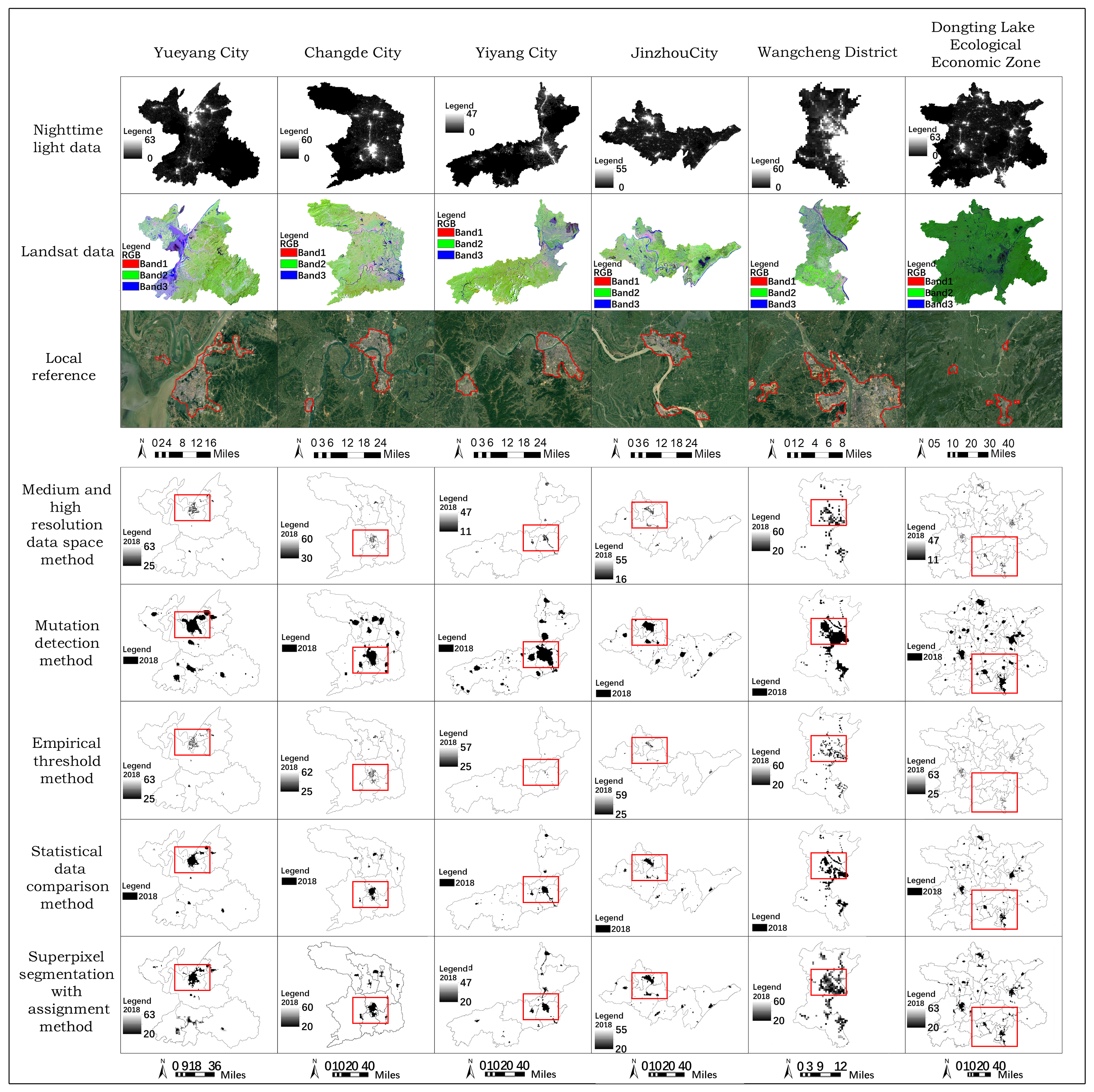
4.2. Extraction Methods Comparison and the UADLEEZ Expansion Display

Based on the 2018 data, we conducted a comparative analysis of the UADLEEZ extraction results with those produced using different methods. As the Figure 7 shows we used the NTL data, Landsat data, the medium and high resolution data space method (MHRDSD), the mutation detection method (MDM), the empirical threshold method (ETM), the statistical data comparison method (SDCM), and superpixel segmentation with assignment method (SSAM) to compare Changde City, Yiyang City, Yueyang City, Jingzhou City, Wangcheng District, and the UADLEEZ, respectively.

The MHRDSD distinguishes between urban and non-urban categories based on higher-resolution data, extracts gray histograms of NTL data, and takes the increasing gray value as the segmentation threshold. We observed that the range of the method extraction is very high, but the method requires a huge amount of data and powerful computer equipment, involves a long extraction times, and has no related verification method. The MDM seeks to determine the side length of the urban built-up area under each threshold. The required process is complicated and the workload is large, which greatly increases the difficulty of extracting the urban built-up area. We found that the final extraction range is larger than the actual built-up area. In the ETM, the extraction threshold is determined based on previous experience and relevant background knowledge. Therefore, the urban built-up areas extraction results vary depending on the subjective influence of researchers, and each range varies greatly due to subjective will. The SDCM uses computer language and adopts the idea of a dichotomy, continuously calculating the area of urban built-up areas under each dynamic threshold and comparing them to statistical data released by relevant departments to extract the threshold. However, the statistical data that this method relies on are not necessarily true values, so there are biases. Nevertheless, SDCM is more accurate than either the MDM or the ETM. The local reference images in Figure 7 are from HD satellite imagery. We circled the urban built-up areas, which correspond to the areas in the red frame of each extraction result. It can be clearly observed that SSAM was closer to the true value than other methods, indicating that it was more accurate. Unlike the above methods, the SSAM requires that researchers have specific programming knowledge and the ability to use multiple software application.

The accuracy of the extracted data was tested. The sampled data were the local range of the Dongting Lake area corresponding to the 2018 Landsat data, and 100 sample points each of the built-up area and the non-built-up area are randomly selected, as shown in Figure 8. Based on this model, the MHRDSD, the MDM, the ETM, the SDCD, and the SSAM were evaluated for sampling accuracy. We used sample data to test the accuracy of five methods, the results are shown in

Table 2. Methods comparative accuracy analysis.

Region	MHRDSD	MDM	ETM	SDCM	SSAM
urban built-up area(OA)	0.803921569	0.743119266	0.791666667	0.858585859	0.861386139
non-urban built-up area(OA)	0.816326531	0.791208791	0.769230769	0.851485149	0.886597938
Kappa	0.62	0.53	0.56	0.71	0.75

.

According to the results of overall accuracy (OA) and Kappa coefficient, it is known that the data extracted from the built-up area using the SSAM has higher precision, indicating that the results of the method of extracting urban built-up area data in this paper are higher than the four classical threshold methods. Reaching the expected goal of refined processing. This method can be used in single or larger areas, which makes it most capable of capturing the reality, and it can be studied continuously for long time periods. Using this method, we not only clearly determined the boundary of the built-up area, but also identified the gray value of noctilucent. Figure 9 shows the annual expansion process of the UADLEEZ built-up area from 1992 to 2018. It authentically reflects the UA expansion and change process. We could observe the changes of cities from the subtle changes, summarize the rules of urban expansion, and have value as a reference for the formulation of subsequent research and planning.

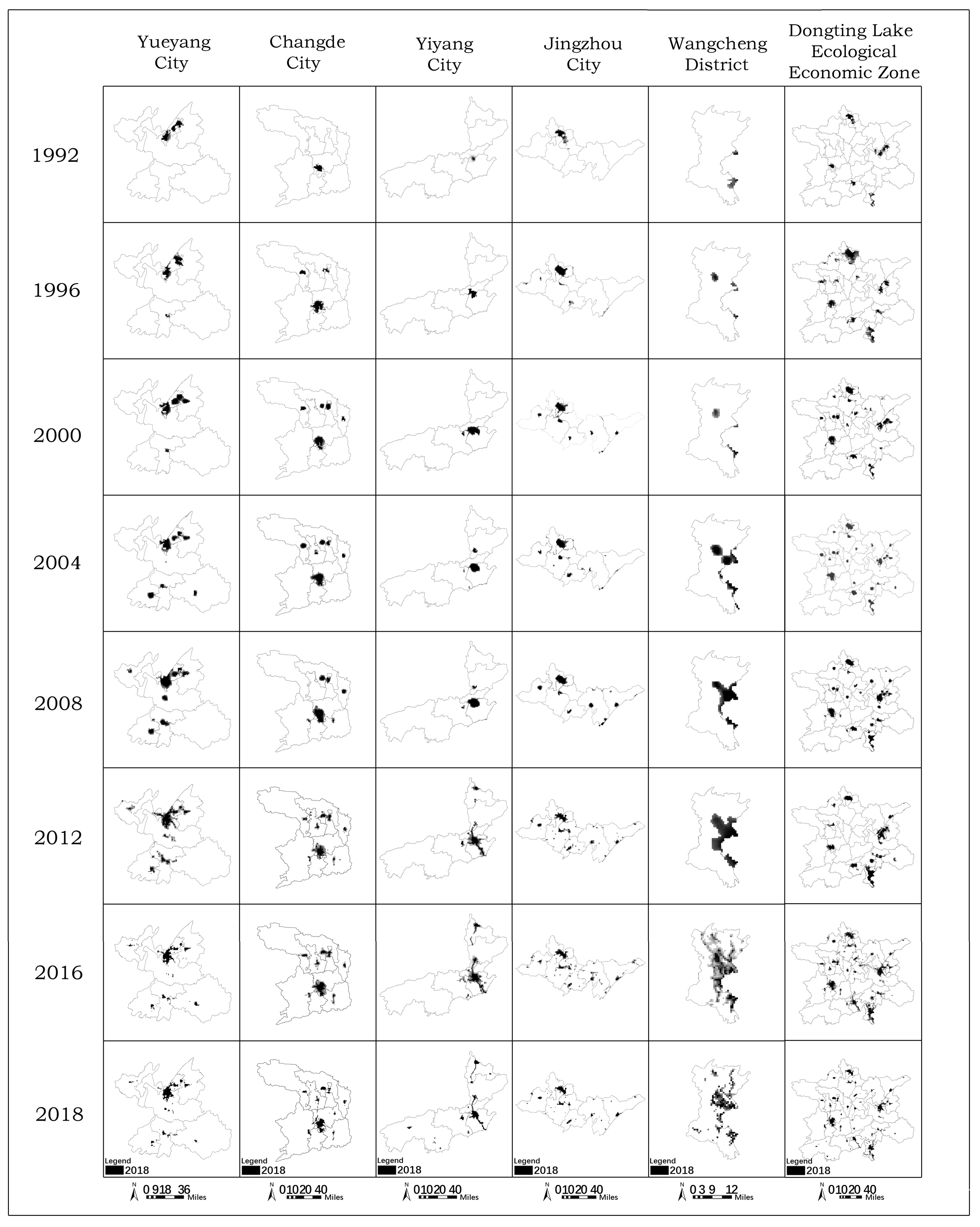
4.3. The UADLEEZ Spatiotemporal Expansion Analysis

4.3.1. Scale Expansion Analysis

Figure 10 shows an extended overlay map of the UADLEEZ from 1992 to 2018. The bottom is a topographic map; blue indicates lower elevations, mainly lakes and low plains, while red indicates higher elevations dominated by hills and mountains. The “horseshoe” terrain features low in the middle and north—near half of the area is less than 50 m—and high in the west, south and east. Dongting Lake swallows the Yangtze River and accommodates four bodies of water. It is a typical over-water lake, with a high, middle, and low lake basin shape. The hydrological characteristics of summer waterlogging and winter dryness have restricted the development of the lake area to a certain extent, and also contributed to the unique spatial form. Natural conditions are the basis for the expansion of UA. Yueyang City, etc., are located on the plains at lower elevations. The terrain is flat and wide, and the conditions are convenient for promoting the rapid development of cities. However, Anhua County, and Shimen County, etc., are located in hillocks and hills. They are mainly mountainous and narrow in areas, which are not conducive to large-scale development and construction. Due to the differences in natural conditions, the urbanization level in the lake area was significantly lower than the average level in Hunan and Hubei province.

We analyzed the spatial and temporal expansion and change process of the UADLEEZ from 1992 to 2018 in terms of expansion area, speed, and intensity. It can be observed from Figure 11 that from 1992 to 2000, except for the sudden increase in the expansion area in 1998, when expansion reached a maximum intensity of 33.8%, the overall trend was decreasing. During this period, the expansion intensity dropped sharply and the expansion speed was slow. From 2000 to 2006, the area and speed of expansion increased in stages, with little change in intensity. Starting from the valley value in 2000, the expansion area and speed were 20.42 km² and 10.21 km²/y, respectively, and the intensity was also at a lower value of 4.5%. The area and speed of urban growth steadily increased to an average level, with little change in intensity and a steady rise. From 2006 to 2014, the expansion followed a “W”-shaped growth pattern, and the growth intensity reached a peak of 3.7% in 2012. During this period, urban growth fluctuated violently, a combination of infill and outward expansion. From 2014 to 2018, the city developed at a high speed, the expansion area and speed reached the peak of 171.19 km² and 85.6 km²/y, respectively, and the expansion intensity showed signs of slowing down. In general, the total area of the region has increased and the expansion speed and expansion intensity have fluctuated, but the area will soon experience a new rising period. Indeed, the UA is likely to face new accelerated development.

From 1992 to 2000, regional expansion occurred in the form of an enclave, separated from the original main urban area and obviously developing in the county. For example, in 1995, the Jingzhou Yihuang Expressway and the Jingsha Railway Xiahe Line were completed and opened to traffic, accelerating the connection between cities and towns and thereby facilitating the development of villages and towns. From 2000 to 2006, the area experienced marginal expansion, extending outward around the original center under the UA effect, which manifested as the “reproduction effect” in patches. The extension speed increased year by year and the area spread irregularly around the patch, based on the increase in the area of a single plaque. In 2004, China formulated the “Industrial Structure Adjustment Guidance Catalogue” and “Interim Regulations on the Direction of Industrial Structure Adjustment.” The main motivation for these policies was that the population gathering had increased social production and living demand, making the area capable of supporting the functions of urban facilities for industrial park expansion and upgrading. From 2006 to 2012, it expanded in a filling manner, and the gray value of the light intensity gathering inside the patch increased. Under the policies of “old city renewal” and “shantytown reconstruction”, the urban area transformed from a state of scattered and disorderly diffusion to one of adjustment, improvement, and optimization of internal functional structures. For example, in 2007, the Yueyang Municipal Government issued a notice to strengthen controls on illegal construction and demolition work in central urban areas. Cities experienced slower horizontal growth, but the vertical growth of spaces increased. From 2012 to 2018, it expanded in enclaves and the spatial distribution was relatively scattered, basically jumping out of existing patches and relying on radioactive expansion of state roads, provincial roads, and water transportation, etc. urban expansion had obvious orientation, accessibility, and planning, enabling the surrounding areas to effectively drive the transfer of functions, land conversion, and expand regional development frameworks, signs of the implementation of a “traffic-led development” strategy in the region. Such as the notice of cement (asphalt) road plan of the natural village in Yiyang City in 2018 construction, the notice of the provincial trunk line construction and the highway construction.

4.3.2. Gravity Center Offset Analysis

To extend our analysis, we drew a spatial-temporal gravity center offset chart. Figure 12a was developed using a simple geometric center method commonly used in previous studies—that is, an unweighted homogeneous luminous center. It can be observed that the offset distance and intensity of (a) was significantly larger than that of (b), and the moving lines and directions are relatively simple. In this study, we used the gray value of the luminous intensity pixel as the weight, and calculated the gravity center of the multi-gray value homogeneous space. The average light intensity of gravity center was not the same. The stronger the light intensity, the closer it was to the downtown area. Figure 12b plots the gravity center offset for the method of adding weights. The law of the space of gravity center movement can be more realistically and intuitively reflected on the road map. The movement was more complex and tighter, which is in line with the reality.

As Figure 12 shows, the gravity center of the UADLEEZ was mainly concentrated in the northeast of the center. As the years progressed, it moved between Shishou City, Huarong County, Nan County, and Yuanjiang City. The north latitude was 29°60′ to 29°0′, and the east longitude was 112°10′ to 112°40′. The gravity center moved from Jingzhou City to Yueyang City through Yueyang City. It can be observed from Figure 12b, from 1992 to 2018, the gravity center moved southward, indicating that development occurred more rapidly in Yueyang City, Yiyang City, and the Wangcheng District than in Jingzhou City and Changde City. However, there were several periods, such as 2014–2017, when a leap to the north, Changde City and Jingzhou City development accelerated in these periods. In the east-west direction, it moved at a distance of about 30′. Before 2003, the gravity center moved slowly from east to west, indicating that Changde City and Yiyang City developed well. After 2003, Yueyang City and Wangcheng District accelerated their development, and the gravity center moved rapidly to the east, reaching the eastern end in 2014; after that, it moved slowly to the west, and development sped up in this region. In 2018, the gravity center fell on Nan County, Yiyang City. As Figure 13 shows, we separately analyzed the gravity centers of the five areas (the four cities and one district); we found that each area tended to move closer to the center year by year, especially after 2014. This indicates that the policy (Dongting Lake Ecological Economic Zone Planning, 2014) promoted regional development and traction made it accumulate.

From 1992 to 2000, the offset distance and velocity slowly decreased, from 22,531.81 m/y to 5101.24 m/y, and the angle shift was relatively severe. In 1994 and 1997, the turning points in the same direction were 147.06° and 112.42°, respectively. During this period, urbanization accelerated and urban areas expanded rapidly; from 2000 to 2006, the movement speed and distance showed two rising climaxes, which were 19,329.94 m/y in 2000 and 15,588.22 m/y in 2003, but reached the minimum offset value of 2870.859 m/y in 2006. The overall change was gentle and the angle change was small. During this time, the speed of urban expansion slowed down, indicating that the city was undergoing internal filling development; from 2006 to 2014, the gravity center migration velocity fluctuated. In 2009, the velocity reached a high value of 17,093.2 m/y and the moving angle was −98.57°. During this period, the cities in the UA developed steadily and relatively stable; the offset distance and velocity were relatively fast from 2014 to 2018, and the angle changed drastically. In 2015, it reached the maximum change angle of 175.04°, the research areas were developed rapidly.

4.3.3. Landscape Pattern Analysis

We used the landscape pattern analysis to examine the regional ecological environment of the UA. As shown in Figure 14, we divided regional landscape pattern indicators into four groups for analysis: (a) to (d) are area edge indicators, (e) to (h) are separation indicators, (i) to (l) are cluster indicators, and (m) to (p) are diversity indicator. In Figure 14 below, several landscape pattern indexes changed dramatically in 2014, because we tried to unify the DN value saturation of NTL data during pre-processing, and the gray value of VIIRS/DNB data is 0–63 Reclassified. The processing results did not meet our expectations. The DN value saturation of the NTL data was consistent, but the spatial resolution of the VIIRS/DNB data is higher than the DMSP/OLS data, and the night light of the VIIRS/DNB are more elaborate, so this huge change occurred.

As the total area (TA) results in Figure 14a show, the landscape area increased steadily, except for in 1998 when the fluctuation reached 35,745.2 ha. The data could be used as the basis for calculating other indicators. As Figure 14b clearly shows, the patch density (PD) value in this area was higher than 0.5, except for in 2013, when it was 0.39. This is a relatively high level, indicating that the landscape fragmentation of the area was relatively large. However, in terms of the entire time period, PD decreased year by year, meaning the degree of fragmentation was gradually decreasing, a good trend for the development of UA. The overall area of perimeter area fractal dimension (PAFRAC) in Figure 14c is above 1.5; it was only around 1.48 in 1997, 1998, and 2001 and it increased in waves year by year, reaching 1.71 in 2017. This shows that the spatial scale shape of the area as relatively complicated and became more complicated under the influence of human activities. Since the method we used in this study can obtain more accurate city boundaries, the patch boundary curve DNB also more accurate and complicated. The landscape shape index (LSI) in Figure 14d fluctuated between 1.3 and 1.56. From 1992 to 2003, there were a small fluctuation and a slow trend towards 1; in 1997, the patch was most regular. During this period, the region transitioned from “quantity growth” to “scale expansion”, and the UA became more compact. After 2004, the patches changed rapidly in complexity. In 2013, the shapes of the patches were the most complicated, and the UA developed rapidly during this period.

The fluctuation range of the interspersion and juxtaposition index (IJI) in Figure 14e was between 78% and 88%, and the overall stability was stable, indicating that the patch distribution was more uniform. Taking 2007 and 2013 as the peak and trough, respectively, we separated the patch distribution changes in three periods to reflect the development of the UA. The overall landscape division index (DIVISION) in Figure 14f was above 0.982, indicating that the landscape patch subdivision index was very high and the landscape fragmentation was serious. These trends are accelerating and better means are needed to plan governance. Effective mesh size (MESH) was based on TA’s corresponding patch size and area-weighted average patch size. In Figure 14g, the area of these patches was relatively small compared to TA. The study period increased from 119.03 ha to 391.33 ha with the year. The splitting index (SPLIT) in Figure 14h showed that the fluctuation of the degree of separation with the change of the year was relatively small, fluctuating in 1998 and remaining stable since then. In other words, the distance separation between the patches remained relatively stable, and the patches were balanced.

Figure 14i shows an overall perspective on the contagion (CONTAG); the regional spread was stable, between 11% and 20%, indicating that the connectivity between landscape patches was low, the layout of landscape elements was scattered, and the landscape was fragmented to a high degree. In 2007, it reached its lowest value of 11.67%. From 1992 to 2007, it trended downward, and after 2007, it trended upward. The period generally extended upwards, and the extension trend and connectivity gradually strengthened. As Figure 14j shows, the percentage of like adjacencies (PLADJ) data gradually climbed from a lower value of 6.87% in 1992 to 26.59% in 2013. The urban development moved from quantity to quality, and the degree of aggregation slowly increased. The patch cohesion index (COHESION) measures the physical connectivity of corresponding patch types. As Figure 14k shows, the physical connectivity was basically lower than 50% initially, a low connectivity level, but it gradually increased as years passed. The connectivity of the region gradually rose from a lower level, and the development of the UA gradually transitioned from independent development to overall development. As Figure 14l shows, the aggregation index (AI) percentages were all lower than 35%, and they fluctuated around 15%; in other words, the degree of regional patch accumulation was low. In general, the agglomeration degree increased over time, indicating that cities were developing increasingly close relationships.

As Figure 14m shows, the comprehensive Shannon’s diversity index (SHDI) value for the study area during the study period was relatively stable at about 3, reaching a maximum of 3.31 in 1994 and a minimum of 2.43 in 2013. This indicates that the land use types were relatively rich, the degree of fragmentation was high, and the information content of uncertainty was large. As Figure 14n shows, Shannon’s evenness index (SHEI) approached 1 in the region, reaching a high value of 0.985 in 2007. There was no obviously advantageous type of landscape with low dominance, and each patch was evenly distributed with high diversity. Figure 14o shows the largest patch index (LPI) during the study period; only 2002 and 2013 were higher than 50%, at 51.9% and 67.5%, respectively. The types and proportions of the largest patches were still relatively small, and they experienced a steady decline, indicating that interference from human activities was intense and highly frequent, affecting the degree of fragmentation and ecological fragmentation. As Figure 14p shows, the patch richness density (PRD) gradually decreased with time, indicating that the growth rate of the landscape area was faster than the quantity growth, and there was no proportional growth. Thus, while the UA expansion occurred via enclave-type expansion, it also occurred through the edge- and infill-type expansion modes.

5. Discussion

5.1. Discussion of UADLEEZ Expansion

The UADLEEZ expansion has resembled most urban development models. During the 27 years covered in this study, the construction land of the UA showed an epitaxial expansion trend, with an average annual growth of 42.11 km², an area growth rate of 423.3%, and an average expansion intensity of 10.04%. The spatiotemporal evolution of the urban system followed a steady outward enclave-type expansion at a medium speed from 1992 to 2000, when the compactness of the UA also decreased; from 2000 to 2006, it underwent high-speed spread edge-type expansion and the compactness continued to decline; from 2006 to 2012, it experienced low-speed fill-type expansion and increased compactness; and from 2012 to 2018, it underwent rapid extension of the enclave-type expansion and the space compactness of the UA declined rapidly. The process of development gradually changing from quantitative growth to scale growth and then back to quantitative growth is cyclical. The spatiotemporal expansion of the UADLEEZ is a three-process cycle, with each process lasting about 5–6 years.

From 1992 to 2003, the gravity center of the UADLEEZ shifted to the southwest (Changde, Yiyang direction); from 2003 to 2014, it shifted to the southeast (Yueyang, Wangcheng direction); from 2015 to 2017, it changed its direction to the northwest (Changde, Jingzhou direction); and finally, in 2018, it moved in a southeast direction (Yueyang, Wangcheng direction). The growth rates of the built-up areas in the region were Changde City > Yueyang City > Jingzhou City > Yiyang City > Wangcheng District. Changde City and Yueyang City led the rapid development of the UA. According to the plan, Yueyang would develop to the west, Jingzhou to the south, Changde to the east, and Yiyang and Wangcheng to the north. The expansion speed of the combination of terrain with good basic conditions is faster, while the expansion speed of the lower plain areas that are easily affected by floods and the higher hilly areas that are more difficult to develop is slower.

The landscape pattern index morphological of the UADLEEZ indicates that the cities and towns in the UA are relatively independent with weak connectivity. There is no large-scale urban sprawl area, and has the characteristic of spatial diffusion. The “five-core” space expansion model is based on the central urban district and the surrounding high-speed expansion areas and counties as the core, and other counties and cities as the edges. The main urban area expansion mode mainly refers to marginal-type expansion, and it extends outward in irregular circles around the original center, as seen in the plaque characteristics of Jingzhou District and Dingcheng District. In recent years, the proportion of enclave-type expansion has increased; the trend of extension along regional traffic arteries and the waters axis is obvious, as seen in Pingjiang and Shimen Counties.

5.2. Discussion of Future Trends in this Region

We collected the planning policies for the nation, Hunan province, Hubei province, and various regions from 1992 to 2018, and used them to analyze the reasons for the expansion. This investigation showed that the results of the above analysis are consistent with the actual situation. After 2014, the UA expanded in size, improved regional functions, strengthened infrastructure construction, and improved urban quality. During this period, the goal among cities was to develop towards an overall regional system, but the situation had not yet coalesced, and the plan did not emphasize coordinated development among cities. Due to the particular characteristics of terrain, topography, and ecological forms, the development mode of the UADLEEZ did not resemble the regional integration of other UAs (such as the Beijing-Tianjin-Hebei UA, etc.). The development model is more suitable for independent urban development that preserves and maintains unique wetland resources and species diversity. However, it remains necessary to strengthen the links between cities, break provincial boundaries, promote the construction of ecological civilization and modern industrial systems, etc., and improve mutual benefits and complementarity.

Due to the complex terrain structure and large span of the UADLEEZ, existing spatial structures need to be optimized, and the construction of related facilities at terrain junctions need to be strengthened. This study found that water and land transportation have played a key role in regional development. Taking Yueyang City as an example, the region has convenient transportation, with Chenglingji port, Guangzhou-Wuhan express railway, Beijing-Guangzhou railway, the Beijing-Hong Kong-Macau expressway, G56 HangRui highway, and other important transportation trunks passing through, so Yueyang City is the most developed city in the region. Therefore, we should pay attention to improving transportation, accelerating the construction of water and land transportation in underdeveloped cities and towns, forming a transportation network system, and achieving the organic combination of high-speed roads, national roads, provincial roads, county roads, and rural roads, which will not only enhance the connectivity among cities and towns within the region, but also facilitate the sharing of resources and the achievement of common development.

To protect the sustainable development and carrying capacity of the UADLEEZ’s ecological resources, industry and population size should be regulated based on the ecological environment’s capacities, the ecological environmental pressure caused by the expansion of the UA should be reduced, and the quality of development should be improved. The development of the UADLEEZ should actively extend north and south direction of the Beijing-Guangzhou railway to connect the Chang-Zhu-Tan UA and the Wuhan urban circle, connect Sanxiang by “four waters”, link the “Yangtze River Delta” and “Pearl River Delta” economic belt, and build a regional development pattern of "lake development, ecological civilization".

6. Conclusions

After analyzing the advantages and disadvantages of current methods, we explored the reasonable use of multi-source data combined with newer technologies, leading us to develop and utilize the SSAM to study 27 consecutive years of UA expansion. We verified the effectiveness of this method in the case of UADLEEZ, showing that the method can extract the urban built-up area in 3.16 s, and the visual extraction of the area is more in line with the actual situation. In the accuracy detection, the Kappa coefficient reaches 0.75, which is more precise than other classic extraction methods. The regional evolution law is consistent with planning, traffic, and policies. The expansion has undergone medium-speed adjustment and enclave-type expansion development, high-speed edge expansion, low-speed internal filling, and a rapid enclave expansion process, showing complex periodic changes. It has expanded following the “five-core” space model, with unique features of regional topography and characteristics of diffusion development. This study provides SSAM that should prove useful for subsequent research, lays the foundation for urban studies, and also provides an important reference for the decision-making of planning departments.

In the following research, we will try to explore two aspects. (1) We will try to apply the proposed method to single-core cities (Changsha, etc.), megacities (Shanghai, etc.), larger regions (the middle reaches of the Yangtze River, etc.), and other countries. (2) We will try to construct a standard data set of the Dongting Lake Ecological Economic Zone to provide a certain reference for future method research and accuracy comparison.

References

1. Seto, K.C.; Fragkias, M.; Güneralp, B.; Reilly, M.K. A meta-analysis of global urban land expansion. PLoS ONE 2011, 6, e23777. [Google Scholar] [CrossRef]
2. Xu, Y.; Yu, L.; Zhao, F.; Cai, X.; Zhao, J.; Lu, H.; Gong, P. Tracking annual cropland changes from 1984 to 2016 using time-series Landsat images with a change-detection and post-classification approach: Experiments from three sites in Africa. Remote Sens. Environ. 2018, 218, 13–31. [Google Scholar] [CrossRef]
3. Pesaresi, M.; Ehrlich, D.; Ferri, S.; Florczyk, A.; Carneiro Freire, S.M.; Halkia, S.; Julea, A.M.; Kemper, T.; Soille, P.; Syrris, V. Operating Procedure for the Production of the Global Human Settlement Layer From Landsat Data of the Epochs 1975, 1990, 2000, and 2014. Publ. Office Eur. Union 2016, 2016, JRC97705. [Google Scholar]
4. Bartholomé, E.; Belward, A. GLC2000: A new approach to global land cover mapping from Earth observation data. Remote Sens. 2005, 26, 1959–1977. [Google Scholar] [CrossRef]
5. Elvidge, C.D.; Tuttle, B.T.; Sutton, P.C.; Baugh, K.E.; Howard, A.T.; Milesi, C.; Bhaduri, B.; Nemani, R. Global distribution and density of constructed impervious surfaces. Sensors 2007, 7, 1962–1979. [Google Scholar] [CrossRef]
6. Melchiorri, M.; Florczyk, A.J.; Freire, S.; Schiavina, M.; Pesaresi, M.; Kemper, T. Unveiling 25 Years of Planetary Urbanization with Remote Sensing: Perspectives from the Global Human Settlement Layer. Remote Sens. 2018, 10, 768. [Google Scholar] [CrossRef] [Green Version]
7. Liu, X.; Hu, G.; Chen, Y.; Li, X.; Xu, X.; Li, S.; Pei, F.; Wang, S. High-resolution multi-temporal mapping of global urban land using Landsat images based on the Google Earth Engine Platform. Remote Sens. Environ. 2018, 209, 227–239. [Google Scholar] [CrossRef]
8. Elvidge, C.; Hsu, F.-C.; Baugh, K.; Ghosh, T. National trends in satellite-observed lighting: 1992–2012. In Global Urban Monitoring and Assessment through Earth Observation; CRC Press: Boca Raton, FL, USA, 2014; pp. 97–120. [Google Scholar]
9. Levin, N.; Duke, Y. High spatial resolution night-time light images for demographic and socio-economic studies. Remote Sens. Environ. 2012, 119, 1–10. [Google Scholar] [CrossRef]
10. Sutton, P.C. A scale-adjusted measure of “urban sprawl” using nighttime satellite imagery. Remote Sens. Environ. 2003, 86, 353–369. [Google Scholar] [CrossRef]
11. Henderson, M.; Yeh, E.T.; Gong, P.; Elvidge, C.; Baugh, K. Validation of urban boundaries derived from global night-time satellite imagery. Remote Sens. 2003, 24, 595–609. [Google Scholar] [CrossRef]
12. Keola, S.; Andersson, M.; Hall, O. Monitoring economic development from space: Using nighttime light and land cover data to measure economic growth. World Dev. 2015, 66, 322–334. [Google Scholar] [CrossRef]
13. Bagan, H.; Yamagata, Y. Analysis of urban growth and estimating population density using satellite images of nighttime lights and land-use and population data. Remote Sens. 2015, 52, 765–780. [Google Scholar] [CrossRef]
14. Zhang, Q.; Seto, K.C. Can night-time light data identify typologies of urbanization? A global assessment of successes and failures. Remote Sens. 2013, 5, 3476–3494. [Google Scholar] [CrossRef] [Green Version]
15. Liu, Z.; He, C.; Zhang, Q.; Huang, Q.; Yang, Y. Extracting the dynamics of urban expansion in China using DMSP-OLS nighttime light data from 1992 to 2008. Landsc. Urban Plan. 2012, 106, 1–72. [Google Scholar] [CrossRef]
16. Zhang, Q.; Schaaf, C.; Seto, K.C. The vegetation adjusted NTL urban index: A new approach to reduce saturation and increase variation in nighttime luminosity. Remote Sens. Environ. 2013, 129, 32–41. [Google Scholar] [CrossRef]
17. Patel, N.N.; Angiuli, E.; Gamba, P.; Gaughan, A.; Lisini, G.; Stevens, F.R.; Tatem, A.J.; Trianni, G. Multitemporal settlement and population mapping from Landsat using Google Earth Engine. Int. J. Appl. Earth Obs. Geoinf. 2015, 35, 199–208. [Google Scholar] [CrossRef] [Green Version]
18. Jie, Y.; Zhang, Y.; Zhong, H. Monitoring urban expansion and land use/land cover changes of Shanghai metropolitan area during the transitional economy (1979–2009) in China. Environ. Monit. Assess. 2011, 177, 609–621. [Google Scholar] [CrossRef]
19. Woodcock, C.E.; Allen, R.; Anderson, M.; Belward, A.; Bindschadler, R.; Cohen, W.; Gao, F.; Goward, S.N.; Helder, D.; Helmer, E.; et al. Free access to Landsat imagery. Science 2008, 320, 1011. [Google Scholar] [CrossRef]
20. Liu, D.; Chen, N.; Zhang, X.; Wang, C.; Du, W. Annual large-scale urban land mapping based on Landsat time series in Google Earth Engine and OpenStreetMap data: A case study in the middle Yangtze River basin. ISPRS J. Photogramm. Remote Sens. 2020, 159, 337–351. [Google Scholar] [CrossRef]
21. Ning, X.; Wang, H.; Zhang, H.; Liu, Y.; Pang, B.; Hao, M. High-Precision Urban Boundary Extraction and Urban Sprawl Spatial-Temporal Analysis in China’s Prefectural Cities from 2000 to 2016. Geomat. Inf. Sci. Wuhan Univ. 2018, 43, 1916–1926. [Google Scholar] [CrossRef]
22. Wang, H.; Ning, X.; Zhang, H.; Liu, Y.; Yu, F. Urban Boundary Extraction and Urban Sprawl Measurement Using High-resolution Remote Sensing Images: A Case Study of China’s Provincial Capital. ISPRS Technol. Remote Sens. 2018, 42, 1862–1868. [Google Scholar] [CrossRef] [Green Version]
23. Jing, W.; Yang, Y.; Yue, X.; Zhao, X. Mapping Urban Areas with Integration of DMSP/OLS Nighttime Light and MODIS Data Using Machine Learning Techniques. Remote Sens. 2015, 7, 12419–12439. [Google Scholar] [CrossRef] [Green Version]
24. Goldblatt, R.; Stuhlmacher, M.F.; Tellman, B.; Clinton, N.; Hanson, G.; Georgescu, M.; Wang, C.; Serrano-Candela, F.; Khandelwal, A.K.; Cheng, W. Using Landsat and nighttime lights for supervised pixel-based image classification of urban land cover. Remote Sens. Environ. 2018, 205, 253–275. [Google Scholar] [CrossRef]
25. Ban, Y.; Jacob, A.; Gamba, P. Spaceborne SAR data for global urban mapping at 30 m resolution using a robust urban extractor. ISPRS J. Photogramm. Remote Sens. 2015, 103, 28–37. [Google Scholar] [CrossRef]
26. Ma, X.; Tong, X.; Liu, S. Optimized Sample Selection in SVM Classification by Combining with DMSP-OLS, Landsat NDVI and GlobeLand30 Products for Extracting Urban Built-Up Areas. Remote Sens. 2017, 9, 236. [Google Scholar] [CrossRef] [Green Version]
27. Han, J.; Li, S.; Zhang, T. Research on Urban Expansion Method Based on Deep Learning of Remote Sensing Image. Manned Spacefl. 2017, 23, 414–426. [Google Scholar]
28. Zhang, P.; Pan, J.; Xie, L.; Zhou, T.; Bai, H.; Zhu, Y. Spatial-Temporal Evolution and Regional Differentiation Features of Urbanization in China from 2003 to 2013. ISPRS Int. J. Geo-Inf. 2019, 8, 31. [Google Scholar] [CrossRef] [Green Version]
29. Shi, K.; Huang, C.; Yu, B.; Yin, B.; Huang, Y.; Wu, J. Evaluation of NPP-VIIRS night-time light composite data for extracting built-up urban areas. Remote Sens. Lett. 2014, 5, 358–366. [Google Scholar] [CrossRef]
30. Wu, X.; Zhang, P. Urban Boundary Extraction by Fusing of DMSP-OLS and Landsat Images. J. Appl. Sci. 2016, 34, 67–74. [Google Scholar] [CrossRef]
31. Ke, W.; Tao, C.; Ma, J.; Liu, Y.; Zou, Z. Research on Unsupervised City Extraction Based on Landsat and DMSP-OLS. Geomat. Spat. Inf. Technol. 2018, 41, 183–186. [Google Scholar]
32. Roychowdhury, K.; Taubenböck, H.; Jones, S. Delineating urban, suburban and rural areas using Landsat and DMSP-OLS night-time images. In Proceedings of the 2011 Joint Urban Remote Sensing Event, Munich, Germany, 11–13 April 2011. [Google Scholar]
33. Tang, L.; Cui, H. Improvement of Urban Construction Land Extraction Method Based on NPP-VIIRS Nighttime Light Data and Landsat-8 Data: A Case Study of Guangzhou City. Geomat. Spat. Inf. Technol. 2017, 40, 69–73. [Google Scholar]
34. Yin, Z.; Li, X.; Tong, F.; Li, Z.; Jendryke, M. Mapping urban expansion using night-time light images from Luojia1-01 and International Space Station. Int. J. Remote Sens. 2020, 41, 2603–2623. [Google Scholar] [CrossRef]
35. Bai, Y.; He, G.; Wang, G. WE-NDBI-A new index for mapping urban built-up areas from GF-1 WFV images. Remote Sens. Lett. 2020, 11, 407–415. [Google Scholar] [CrossRef]
36. Wang, K.; Li, Z.; Zhang, J. Built-up land expansion and its impacts on optimizing green infrastructure networks in a resource-dependent city. Sustain. Cities Soc. 2020, 55, 102026. [Google Scholar] [CrossRef]
37. Pekel, J.-F.; Cottam, A.; Gorelick, N.; Belward, A.S. High-resolution mapping of global surface water and its long-term changes. Nature 2016, 540, 418–422. [Google Scholar] [CrossRef] [PubMed]
38. Huang, X.; Schneider, A.; Friedl, M.A. Mapping sub-pixel urban expansion in China using MODIS and DMSP/OLS nighttime lights. Remote Sens. Environ. 2016, 175, 92–108. [Google Scholar] [CrossRef]
39. Chen, Y.; Ge, Y.; An, R.; Chen, Y. Super-Resolution Mapping of Impervious Surfaces from Remotely Sensed Imagery with Points-of-Interest. Remote Sens. 2018, 10, 242. [Google Scholar] [CrossRef] [Green Version]
40. Tu, W.; Hu, Z.; Li, L.; Cao, J.; Jiang, J.; Li, Q.; Li, Q. Portraying Urban Functional Zones by Coupling Remote Sensing Imagery and Human Sensing Data. Remote Sens. 2018, 10, 141. [Google Scholar] [CrossRef] [Green Version]
41. Zhou, Y.; Smith, S.J.; Elvidge, C.D.; Zhao, K.; Thomson, A.; Imho, M.A. Cluster-based method to map urban area from DMSP/OLS nightlights. Remote Sens. Environ. 2014, 147, 173–185. [Google Scholar] [CrossRef]
42. Bennett, M.M.; Smith, L.C. Advances in using multitemporal night-time lights satellite imagery to detect, estimate, and monitor socioeconomic dynamics. Remote Sens. Environ. 2017, 192, 176–197. [Google Scholar] [CrossRef]
43. Zhou, Y.; Wang, Y. Extraction of impervious surface areas from high spatial resolution imageries by multiple agent segmentation and classification. Photogramm. Eng. Remote Sens. 2008, 74, 857–868. [Google Scholar] [CrossRef] [Green Version]
44. Hu, X.; Qian, Y.; Pickett Steward, T.A.; Zhou, W. Urban mapping needs up-to-date approaches to provide diverse perspectives of current urbanization: A novel attempt to map urban areas with nighttime light data. Landsc. Urban Plan. 2020, 195, 103709. [Google Scholar] [CrossRef]
45. Shi, L.; Zhong, T. The Spatial Pattern of Urban Settlement in China from the 1980s to 2010. Sustainability 2019, 11, 6704. [Google Scholar] [CrossRef] [Green Version]
46. Tu, B.; Zhou, C.; He, D.; Huang, S.; Plaza, A. Hyperspectral classification with noisy label detection via superpixel-to-pixel weighting distance. IEEE Trans. Geosci. Remote Sens. 2019, 10, 2961141. [Google Scholar] [CrossRef]
47. Tu, B.; Zhang, X.; Kang, X.; Wang, J.; Benediktsson, J.A. Spatial Density Peak Clustering for Hyperspectral Image Classification with Noisy Labels. IEEE Trans. Geosci. Remote Sens. 2019, 57, 5085–5097. [Google Scholar] [CrossRef]
48. Tu, B.; Yang, X.; Li, N.; Zhou, C.; He, D. Hyperspectral Anomaly Detection via Density Peak Clustering. Pattern Recognit. Lett. 2020, 129, 144–149. [Google Scholar] [CrossRef]
49. Song, Y.; Chen, B.; Kwan, M. How does urban expansion impact people’s exposure to green environments? A comparative study of 290 Chinese cities. J. Clean. Prod. 2020, 246, 119018. [Google Scholar] [CrossRef]
50. Al, R.; Shaikh, A.; Liu, W. Quantifying Spatiotemporal Patterns and Major Explanatory Factors ofUrban Expansion in Miami Metropolitan Area During 1992–2016. Remote Sens. 2019, 11, 2493. [Google Scholar] [CrossRef] [Green Version]
Figure 1. The flowchart of the proposed superpixel segmentation with assignment method. (a) Oringinal Landsant data, Band selectiion, 753 band combination, Matched resolution, Processed Landsat Data; (b) Nighttime light data, Superpixel segmented Landsat Data.
Remotesensing 12 01797 g001
Figure 2. Map of study area in China.
Remotesensing 12 01797 g002
Figure 3. From image (ap) are band 321, 345, 432, 453, 541, 543, 562, 564, 571, 632, 652, 743, 752, 753, 764, 765 composition in 2017, respectively.
Remotesensing 12 01797 g003
Figure 4. 2012 comparison of optimal threshold percentage segmentation parameter settings.
Remotesensing 12 01797 g004
Figure 5. 2012 comparison of superpixel block size parameter settings.
Remotesensing 12 01797 g005
Figure 6. 2012 and 2018 comparison of distance algorithm parameter settings.
Remotesensing 12 01797 g006
Figure 7. Extraction results comparison.
Remotesensing 12 01797 g007
Figure 8. Sample of accuracy test data.
Remotesensing 12 01797 g008
Figure 9. 27-year spatiotemporal expansion of UADLEEZ (four cities and one district).
Remotesensing 12 01797 g009
Figure 10. (a) Shows a 27-year expanded overlay map, (b) shows an expanded road traffic map.
Remotesensing 12 01797 g010
Figure 11. An expandsion area, speed, and intensity line chart.
Remotesensing 12 01797 g011
Figure 12. (a) Shows weightless gravity center offset, (b) shows weight gravity center offset.
Remotesensing 12 01797 g012
Figure 13. Weighted gravity center offset map of four cities and one district.
Remotesensing 12 01797 g013
Figure 14. Analysis chart of 16 kinds of landscape index polylines.
Remotesensing 12 01797 g014