Article

Uncertainty in Parameterizing Floodplain Forest Friction for Natural Flood Management, Using Remote Sensing

by
Alexander S. Antonarakis
1,* and
David J. Milan
2
1
Department of Geography, School of Global Studies, University of Sussex, Brighton BN1 9QJ, UK
2
Department of Geography, Geology and Environment, University of Hull, Hull HU6 7RX, UK
*
Author to whom correspondence should be addressed.
Remote Sens. 2020, 12(11), 1799; https://doi.org/10.3390/rs12111799
Submission received: 7 April 2020 / Revised: 22 May 2020 / Accepted: 28 May 2020 / Published: 2 June 2020
(This article belongs to the Section Remote Sensing in Geology, Geomorphology and Hydrology)

Abstract

:
One potential Natural Flood Management (NFM) option is floodplain reforestation or manage existing riparian forests, with a view to increasing flow resistance and attenuate flood hydrographs. However, the effectiveness of floodplain forests as resistance agents, during different magnitude overbank floods, has yet to be appropriately parameterized for hydraulic models. Remote sensing offers high-resolution datasets capable of characterizing vegetation structure from a variety of platforms, but they contain uncertainty. For the first time, we demonstrate uncertainty propagation in remote sensing derivations of complex vegetation structure through roughness prediction and floodplain flow for extreme flows and different forest types (young and old Poplar plantations, young and old Pine plantations, and an unmanaged riparian forest). The lowest uncertainties resulted from terrestrial and airborne lidar, where airborne lidar is currently best at defining canopy leaf area, but more research is needed to determine wood area. Mean literature uncertainties in stem density, trunk diameter, wood, and leaf area indices (20, 10, 30, 20%, respectively) resulted in a combined Manning’s n uncertainty from 11–13% to 11–17% at 2 m to 8 m flow depths. This equates to 7–8% roughness uncertainty per 10% combined forest structure uncertainty. Individually, stem density and trunk diameter uncertainties resulted in the largest Manning’s n uncertainty at all flow depths, especially for flow though Pine plantations. For deeper flows, leaf and woody areas become much more important, especially for unmanaged riparian forests with low canopy morphology. Forest structure errors propagated to flow depth demonstrate that even small flows can change by a decimeter, while deeper flows can change by 40 cm or more. For flow depth, errors in canopy structure are deemed more severe in flows depths beyond 4–6 m. This study highlights the need for lower uncertainty in all forest structure components using remote sensing, to improve roughness parameterization and flood modeling for NFM.

Graphical Abstract

1. Introduction

River flooding between 1987–2017 has killed an estimated 665,000 and displaced 628 million people worldwide, while extreme events (>100 year recurrence interval) account for 290,000 deaths and 265 million displaced people [1]. Climatic changes may increase the risk and impact of flooding, where the global exposure to extreme flooding with a 2 ℃ and 4 ℃ increase rises by around 3.4 and 7.7 times to 27 and 62 million people, respectively [2]. Land use change, such as deforestation, agricultural practices, artificial drainage, and urbanization, has also been shown to increase hydrograph peaks [3,4]. Traditionally, hard engineering solutions have been applied to many floodplains to reduce flood risk. However, these approaches have well documented negative impacts to a river’s sediment budget [5,6], environment and ecology [7,8,9], and in aggravating flooding downstream [10,11]. Natural Flood Management (NFM) practices have recently gained traction and have been promoted by governments [12,13] as a sustainable alternative to hard engineering practices. NFM aims to create interconnected river channels, floodplains and catchments that serves to reduce flooding, improve sediment and nutrient transfer, and improve biodiversity, carbon sequestration, and water quality [12]. Forests have been recognized by, e.g., the European Water Framework Directive and the Forestry Commission, as an important medium in reducing flood risk and mitigating floodwater impact [14,15,16]. However, the scientific underpinning is still limited in determining the impact of NFM measures on the fluvial system once implemented, confirmed recently with the UK Natural Environmental Research Council’s 2017 call in improving our understanding of the effectiveness of NFM (https://nerc.ukri.org/research/funded/programmes/nfm/). The science and message to policy concerning forest effects on flooding have been conflicted [17], especially in relation to the magnitude of flow and the complexity of the system at large spatial scales, such as studies stating that forests cannot effectively delay large-scale floods in larger river systems [18,19]. Yet, most of these considerations have not largely focused on riparian nor floodplain forests, nor accurately describing their structural frontal area to flow.
Floodplain and riparian forests attenuate flow once a flood event is underway, and they can retain and delay water [20]. Floodwater energy is reduced through contact with trunks, branches, and foliage of forests with different densities, ages, and species [21,22,23,24]. The significance of plant-flow interactions has been recognized in recent years but has largely focused on applications to rigid cylinders or shorter vegetation [25,26]. There is the need to create a framework for forest roughness parameterization in hydraulic models that allows the effects of various reforestation scenarios upon flood mitigation to be assessed and facilitate flood simulation for current regenerated floodplains. Current hydrological models allow the evaluation of flow resistance as a function of plant spacing, diameter, and height of vegetation [27,28,29] but do not provide for the complexity of vertical plant frontal area. The parameterization of vegetation and especially woody vegetation in hydraulic models needs to consider the complex structure of plants and their flexibility under flow, particularly when considering more extreme flooding where floodwater can enter tree canopies (e.g., Reference [23,24,30,31,32]). Linking remote sensing derived forest structure with hydraulic model parameterization is an essential step when simulating flow over large river reaches. This is because remote sensing is capable of measuring forest attributes at larger spatial scales compared with ground-based forest inventories and can obtain information on complex tree branching and leaves that is otherwise difficult to obtain by conventional forest inventories. Recent advances in ground and airborne remote sensing have resulted in varying accuracies of predicted forest structural metrics, such as stem spacing, trunk diameters, wood areas, and leaf areas. Yet, it is unclear how important these errors in forest structure are in predicting roughness, as well as which errors can most effectively be reduced.
Quantifying how vegetation blocks flow in complex vegetative environments is an essential step to then investigate what type, distribution, density, structure, and management of forests is needed on a floodplain to effectively reduce the impact of flooding. Floodplain forests in temperate Europe and North America have been dominated by broadleaf forests [33,34]. Their composition and structure are controlled by differences in floodplain elevation, which controls the period of flood inundation, and by variations in floodplain morphology, including features, such as natural levees, paleochannels, and ridge and swale topography. Pioneer stands of Populus and Salix, found in the most active areas of the channel, are subject to active fluvial processes, such as bank erosion, bar evolution, and sediment deposition. Further away from the river channel, mixed broadleaf forests grow on well-drained mineral soils, including Ulmus, Quercus, Fraxinus, and Alnus. This type of forest would usually be inundated by winter and larger magnitude floods. In some ecosystems, conifers, such as Pinus, can be found in wet to drained areas of floodplains (e.g., Pinus sylvestris [35]) or can even be present in the poorly drained riparian zone (e.g., Pinus taeda).
Equations to calculate the friction effects of vegetation require complex and depth-dependent information on vegetation structure. Much of this input data is best attained using remote sensing technologies. This paper investigates uncertainty propagation in remote sensing-based estimates of forest structure, including stem, branch, and leaf area, through roughness prediction for different forest types and for potentially extreme flows. We (1) compile literature-based uncertainty in determining vegetation structural components necessary in predicting roughness, using remote sensing; (2) use an equation for vegetation roughness parametrization for simulating flow through forest stands, incorporating stem density, trunk diameter, wood area index (WAI) and leaf area index (LAI); and (3) quantify and propagate levels of uncertainty in predicting roughness in forested floodplains necessary for numerical modeling of floodplain forest friction. For this analysis, uncertainty propagation will be presented in two stages; (a) roughness uncertainty resulting from uncertainty in remote-sensing estimates of forest structure and (b) demonstrate flow uncertainty (discharge, velocity, and flow depth) resulting from roughness uncertainty in two test floodplain cross-sections. The paper finally seeks to make recommendations to advance the science behind vegetation roughness parameterization in hydraulic models linked to remote sensing data.

2. Literature Uncertainty in Remote Sensing-estimated Forest Structure

Uncertainty from the literature in deriving forest structure variables using remote sensing is reported in this study to quantify levels of uncertainty in predicting roughness. The four main forest structure components considered in this study are stem density or stem spacing, diameter at breast height, woody, and leafy areas. These are provided in Table 1 and Table 2, where Table 1 presents literature estimated stem density and trunk diameter uncertainty using various remote sensing instruments and platforms, and Table 2 gives uncertainties associated with remote sensing studies deriving LAI and WAI. The uncertainties given in these tables are the reported percentage root mean square errors. A number of studies were investigated using terrestrial laser scanning, small- and large-footprint airborne lidar, UAV lidar, photogrammetry, radar, and multispectral imagery.

2.1. Trunk Diameters and Trunk Position

Higher resolution remote sensing platforms that can enter the understory are the best at determining trunk diameters and stem density. Terrestrial Laser Scanning (TLS) offers the rapid collection of very dense three-dimensional point cloud datasets of desired surfaces, which is less time consuming than traditional ground surveying. TLS is a non-invasive technique and can provide a digital and multi-temporal spatial record of forest structure. Good coverage from various scanning angles can optimize the information that could be extracted and reduce TLS’s issue of occlusion (see Reference [36]). Stem detection and spacing estimated from TLS can vary, depending on the forest stand density, with 80–100% detection for a sparse plot (200–400 stems/ha) and 70% for dense plots (500–1500 stems/ha) using single scans [36]. Reference [37] achieved 13–37% detection uncertainty in stands less than 1000 stem/ha with multiple scans, and Reference [38] achieved <13% detection uncertainty for stands between 212–400 stem/ha. In very dense riparian stands (e.g., >2000 stems/ha), where the canopy can start near the ground, the trunk detection could be as low as 60%, even with multiple scans [39] (see Table 1).
Trunk diameter estimation using TLS has reported root mean standard errors (RMSEs) of up to 5.9 cm (21%) (see Table 1). Uncertainties of 1.5–5.9 cm in trunk diameter have been determined from single TLS scans for varying stand densities of 212–1042 stems/ha [38,40,41]. Multiple scans have resulted in lower absolute uncertainty of up to 2.39 cm [37,42,43] but translate to percent uncertainty, again, of around 20%.
Airborne techniques can derive metrics for larger areas than TLS. Prior to the extensive use of lidar, very-high-resolution (<1 m) airborne multispectral data or air photographs were used (e.g., Reference [44,45,46]) with detection uncertainty of 10–20% for overstory trees in organized temperate forests. Airborne techniques have been widely applied to sparse stands or plantations, with overstory tree detection uncertainty usually <30% (e.g., Reference [47,48,49]). Reference [50] used variable search window methods and identified 65–98% of trees in stands of 200–1200 stems/ha. Reference [51], using large footprint, full-waveform lidar determined the density of trees in stands of 500–1400 stems/ha with 6–34% uncertainty. High tree detection uncertainties have also been determined from UAV lidar (e.g., Reference [52], with 8–20%), as well as photogrammetry (e.g., Reference [53], with <13%]. Recent work has also detected overstory tropical crowns [54].
Individual trunk diameters estimated allometrically from lidar detection and delineation methodologies have determined RMSEs up to 21% and R2 > 0.75 [55,56,57,58]. Reference [50] determined a similar RSME for floodplain plantations (10–20%). Using larger footprint lidar, quadratic mean trunk diameter, or basal area have been extracted from single or multiple lidar height intervals [59,60,61,62] or in combination with radar interferometry [63]. Full tree size distributions have been derived recently using full waveform airborne [51] and satellite lidar [64], estimating plot trunk diameter to RMSEs 2.45–5.7 cm (12–31%).
Overall, the uncertainty range reported in the literature (Table 1) is 0–40% for stem spacing and 0–30% for trunk diameter. Average uncertainties are around 20% for stem spacing and 10% for trunk diameter, when obtained using TLS and small footprint lidar.

2.2. Branches and Leafless Structure

Terrestrial Laser Scanning (TLS) is currently the most widely used remote sensing method in determining real complex woody structure with centimeter-millimeter resolution. This is done through scanning an individual tree or a set of trees with their leaves-off, or scanning with leaves-on using a dual-wavelength TLS and subsequently removing the leaves through post-processing the point cloud. TLS has the ability to detect trunks, branches connected to trunks, and even lower order branches [36]. It is noted that smaller branches can make a significant contribution to the total woody surface area [66]. The point cloud of TLS returns needs to be aggregated to a solid surface to determine wood area, e.g., complex meshes [23], voxels [23,67,68,69], or Quantitative Structure Models method [43,70]. Dual-waveform lidar, such as Echidna [71], are now growing in capability to separate trees and branches, if scanning leafless trees is not an option, e.g., for evergreen trees.
Literature on branch surface area from TLS or other remote sensing instruments is limited (Table 2). Reference [72] determined stem surface area with 10% uncertainty, and Reference [23] observed a 40% different between complex meshing and voxel methods to determine branch surface area of riparian poplars. Branch volume has been estimated by, e.g., Reference [73,74], with up to 34% uncertainty. Total tree volume including stems and branches has been estimated to around 24% uncertainty [75]. Crown and branch biomass have also been estimated using TLS to uncertainties of 23–38% [76,77], and total biomass has been estimated by Reference [43] with an uncertainty of 16%.
With the caveat that few branch area studies using remote sensing have been reported, the uncertainty range from Table 2 are up to 40% and an average uncertainty of around 30%.

2.3. Foliage Structure

Vertical foliage profiles are difficult to measure in the field (e.g., Reference [68,78]). Terrestrial Laser Scanning (TLS) has been used to determine LAI and vertical foliage profile. Reference [79] was one of the first to determine a gap fraction from TLS. The gap fraction, or the percentage transmission of light through the canopy can be used to estimate LAI through the Beer–Lambert law (e.g., Reference [24]). Hemispherical projection techniques are also used with the Echidna TLS [80]. Other methods have used voxelization of leafy trees [68]. Using TLS to determine LAI (Table 2) has resulted in uncertainties of between 7–46% and, for LAI, ranges of 0.2–6.5 [81,82,83,84].
Airborne lidar has been used in the recent past to determine vertical profiles of foliage. One approach, using discrete lidar (point clouds) is to simply calculate the ratio of the number of returns below the canopy and within the canopy, providing an estimate of the canopy light transmittance [85,86]. Using small footprint lidar (Table 2), LAI uncertainties have been reported between 6–29% for LAI ranges of up to 12 [87,88,89,90,91,92]. Reference [93,94] developed an equation to extract the vertical gap distribution from full waveform lidar, incorporating all energy returned from all heights within the canopy and from the ground. Use of waveform lidar (Table 2) has produced total LAIs to < RMSE 0.9 m2/m2 or 20% uncertainty in a temperate forest [51] and RMSE 1.36 m2/m2 or 25% uncertainty in a tropical forest [95]. LAI profile problems may occur in areas with uneven topography, or in LAIs > 8 if the ground return energy is low [92,95]. Radar and specifically interferometric radar has been used to create vertical profiles, and through combinations with hyperspectral or lidar, have been able to determine a foliage profile (see Reference [96,97,98]), with resulting LAI uncertainties of 15% (Table 2; Reference [98]).
In general, the uncertainty ranges from the literature (Table 2) are 0–30% for LAI. Average uncertainties are around 20%, with low uncertainties for all remote sensing techniques investigated, i.e., TLS, airborne lidar, and radar.

3. Method

We calculate vegetative roughness of trunks, branched and leaved elements until theoretical full-submergence of trees, incorporating flexibility of branches and leaves, using the Darcy–Weisbach equations and translating them to Manning’s n. To this end, we use an equation for vegetation roughness parametrization for flow through a forested environment, including stem spacing, trunk diameter, WAI, and LAI from Reference [31,32]. Remote sensing is best able to derive complex forest structure when simulating flow over larger river reaches compared to field campaigns. We explore the effects of propagating various levels of uncertainty in predicting roughness in a series of test forest types: young and mature poplar plantations, young and mature pine plantations, and an unmanaged riparian forest, using literature forest structure uncertainty from Section 2. We then demonstrate a second stage error propagation, when the resulting uncertainty in predicting roughness is propagated through flow uncertainty (discharge, velocity, and flow depth) in two test floodplain cross-sections.

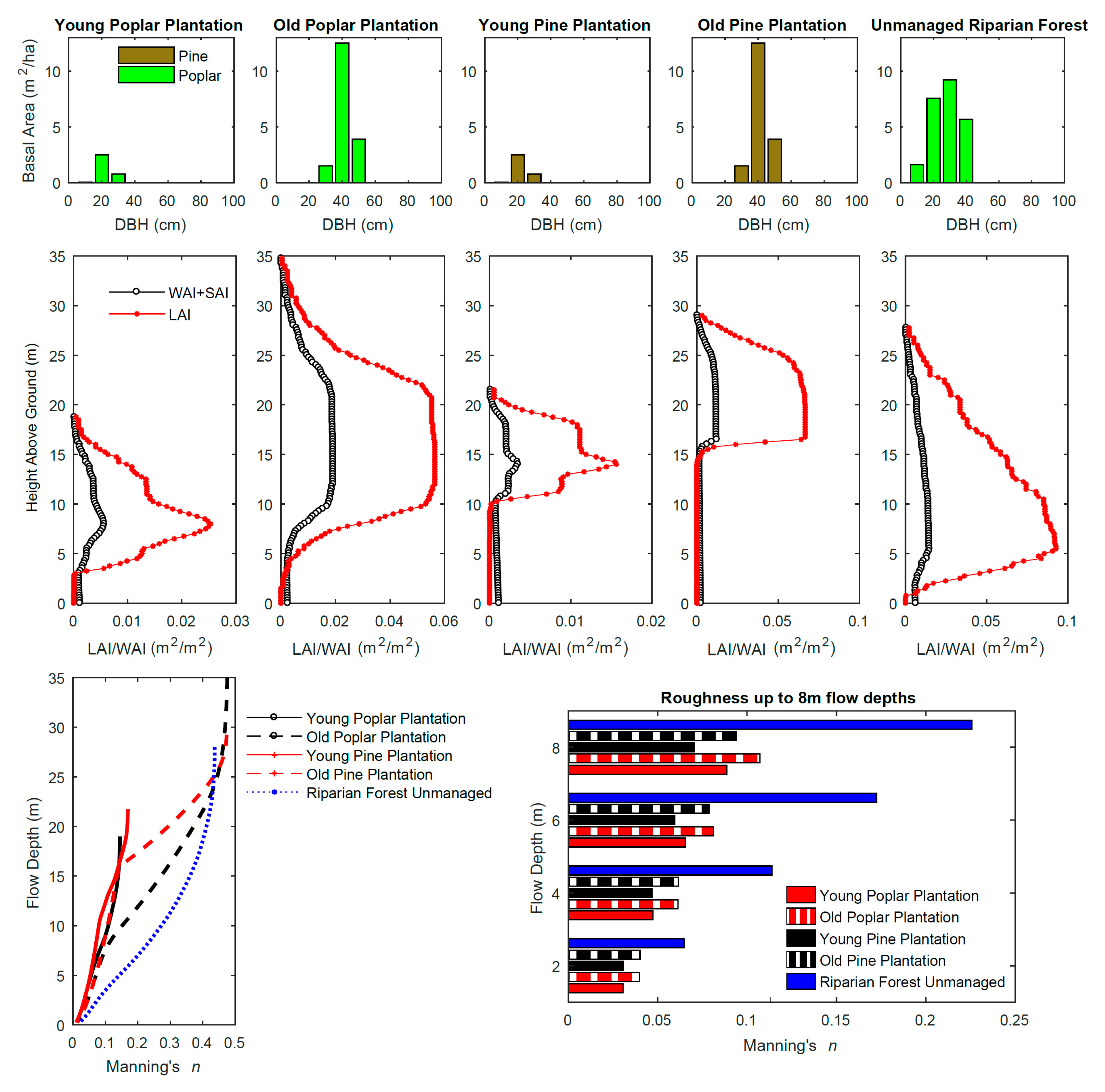
3.1. Vegetation Roughness of a Forest Stand

Darcy–Weisbach equations representing vegetative roughness of trunks, as well as branched and leaved elements, are chosen for this study, presented in Reference [22,31,32,105,106]. These Equations (1) accommodate for incorporation of plant frontal area of bark, branches, and leaves until full submergence of vegetation; (2) are thus conducive to linking with remote sensing derivations of forest structure when large-scale numerical flood simulations are desired; and (3) factor in flexibility of natural riparian plant canopies in flow. Our study uses the friction factor equation presented in Equation (5) from Reference [32], which combines the stem and leaves into a single equation, incorporating the species-specific drag coefficient (Cdi) and the species-specific deformation parameter (χi) for both leaves and stems. In our study, we annotate the friction factor for a whole forested stand ( f s t a n d ( h , x ) ) to more appropriately define stem frontal area as a rigid stem and flexible branches (as a WAI), as well as accommodate for different species in a stand. Theoretical information and more detailed derivation of rigid trunk roughness, as well as flexible branch and flexible leaf roughness, are presented in the Supplementary Materials. The final friction at flow depth (h) over the entire water column and at location x is:
f s t a n d ( h , x ) = 4 [ i ( C d i , T   S A I i ( h , x ) ) + i ( C d i , W ( U c ( x ) U χ i , w ) χ i , w W A I i ( h , x ) ) + i ( C d i , F ( U c ( x ) U χ i , f ) χ i , f L A I i ( h , x ) ) ] .
Here, the rigid stem component ( C d i , S S A I i ( h , x ) ) is calculated from the stem drag coefficient (Cdi,S), and the one-sided area sum of all stems in a plot x ( S A I i ( h , x ) ), with references to flow depth h, of a certain species i per unit area. The derivation of Cdi,S is given in the Equation (S4) and depends on the stem diameter and spacing [107]. The W A I i ( h , x ) considers the frontal projected area of woody branches and twigs of a certain species i per unit area. C d i , W is the species-specific drag coefficient, and χ i , w is the species-specific deformation parameter for branched elements. Here, the total woody friction is calculated as the sum of all trees of all species within a plot. The L A I i ( h , x ) considers the frontal projected area of leaves of a certain species i per unit area. C d i , F is the species-specific drag coefficient, and χ i , F is the species-specific deformation parameter for leaved elements. Again, the total leafy friction is calculated as the sum of all trees of all species within a plot. U χ i , w and U χ i , f are the lowest velocity used in determining χi and is typically 0.1–0.2 m/s, and U c is the depth-averaged mean cross-sectional velocity.
Once the trunk diameters, stem density, WAI, LAI, χw, χf, and drag coefficients have been derived or estimated, Equation (1) can be solved iteratively to estimate f s t a n d ( h , x ) for a desired flow depth. In the first iteration, an initial estimate for velocity U c is provided, if it is unknown, for a certain depth of flow. The resulting first-estimate friction factors calculated from Equation (1) is then input into the Darcy–Weisbach equation to calculate a new velocity given as:
U c = 8 g h S f .
The acceleration due to gravity (g) is 9.81 m/s2, and the slope of the channel (S) can be measured for each specific reach. The new velocity calculated in Equation (2) is replaced in Equation (1) to calculate a new friction factor. This process is repeated until the velocity does not change. The converged velocity is then used to calculate the final resistance for a specified flow depth (see Reference [22,32]). Darcy–Weisbach’s friction factor f can be converted to Manning’s n [105] as:
n = f   ( h 1 / 3 8 g ) .

3.2. Quantification of Forest Structure Uncertainty in Predicting Roughness

3.2.1. Test Forest Types and Control Forest Structure

Poplars are early-successional species that have formed the fabric of wet riparian woodlands due to their ability to withstand seasonally wet hydrological conditions. Poplar plantations are common on floodplains throughout Europe since the 1950s, especially in France, Spain, and Italy [108,109]. It has been estimated that poplar plantations are almost 40 times more abundant globally than willow plantations [110]. Scots pine is one of the most widely distributed trees in Northern Europe and encompasses 20% of the productive forest area of the EU [111]. In the UK, it is the second most abundant commercial conifer, where conifers account for 95% of all forest products [112]. Although Scots Pine is not necessarily a typical riparian forest species, it is evident on floodplains in Scotland, appearing on the River Spey and Feshie [33]. Furthermore, as part of managing and restoring Scotland’s native forest, Caledonian Scots Pine is being actively planted on floodplains in Scotland [35,113]. New native woodlands are also being planted in upland areas in Scotland as part of slow-the-flow projects, where Scots Pine is one of the suitable species being used [114]. Furthermore, beyond the strong presence of pines in floodplains in Scotland, and its dominance in commercial plantations in Northern Europe, the relevance of this species in our study is also that it typifies plantation forests with high canopies, where extreme flooding will not likely come into contact with foliage.
In this study, five test forest types are presented; Young Poplar Plantation, Old Poplar Plantation, Young Pine Plantation, Old Pine Plantation, and Unmanaged Riparian Forest. The Poplar Plantations and Unmanaged Riparian Forest (Populus nigra and Populus deltoides hybrids) are real forests measured in June 2006 in the Garonne River floodplain near Verdun-sur-Garonne, France (UTM31; 359500E 4854000N and 356000E 4861500N; see Reference [23,24]). The Young Plantation contained 86 trees all less than 8 years old, in a plot of 4260 m2; the Mature Plantation contained 110 trees all older than 10 years, in a plot of 5930 m2; and the Unmanaged Riparian Forest contained 234 trees in a plot of 2070 m2. Measurements included trunk diameter, stem number, tree height, and trunk height for all trees greater than 3 cm in trunk diameter. The pine plantations considered in this study are identical to the poplar plantations in terms of trunk diameter and stem density, but have different trunk and tree heights based on Scots Pine (Pinus sylvestris). Tree height was calculated as H = 3.935 × diameter at breast height (DBH)^0.531 and trunk height as Htrunk = H × (0.817-0.0048*DBH-0.00002 × DBH^2), following Reference [115]. Trunk frontal area is defined as the surface areas of trunks until the trunk height.
WAI for the forest types was determined from metabolic scaling theory. The metabolic scaling theory, or West Brown Enquist model [116,117], is based on determining woody structure from branch (RB), diameter (RD), and length (RL) ratios between mother and daughter branches, which, for conifers, is defined as RB =5; RD = RB−0.5; RL=RB−1/3; and, for deciduous trees, RB =3. For poplars, Reference [23] defined branching ratios of RB =3.363; RD = RB−0.429; RL=RB−0.281. To compute the total branched area, as in Reference [22], the initial trunk diameters, finest twig diameter (1 cm in this study), and trunk length need to be defined. The one-sided wood area is defined as half of the product of all branches in each daughter branch order, with their diameters and lengths. The projected area with height was then linearly interpolated from the trunk height to the tree height, i.e., the crown. WAI is then calculated by taking the total one-sided wood area of all trees and dividing by the plot area.
LAI was calculated based of DBH and specific leaf area (SLA): L A I = S L A × a r e a p l o t × ( β D B H α ) . For Scots Pine, β = 0.0065, α = 2.363, and SLA = 5 [118,119,120], and for Poplar β = 0.0114, α = 2.026, and SLA = 14 [121,122,123]. Again, the LAI with height was then linearly interpolated from the trunk height to the tree height. Resulting WAI was 0.172, 1.361, 0.079, 0.489, 0.917 m2 m−2, and LAI was 0.736, 3.997, 0.385, 2.724, 5.306 m2 m−2, for Young and Old Poplar Plantations, Young and Old Pine Plantations, and an Unmanaged Riparian Forest, respectively.

3.2.2. Predicting Roughness and Incorporating Forest Structure Uncertainty

Using Equations (1)–(3), Manning’s n is calculated using the control forest structure described above. The drag coefficients for woody and leaf area ( C d i , W and C d i , F ) can either be determined using experimental studies or through literature. In this study, C d i , W is defined as 0.95 for both pines and poplars, and C d i , F is given as 0.57 and 0.33 for pine and poplar from Reference [31,124]. The species-specific deformation parameter for branches and leaves χ i , w and χ i , f were also obtained from Reference [31,124], where χ w is −0.27 for both pines and poplars, and χ f is given as −0.44 and −1.03 for pine and poplar. The lowest velocity Uχ is defined as 0.2 m/s as in Reference [124], and Uc was initially set to 1 m/s. The slope of the channel (S) in Equation (2) was set to a value of 0.001, chosen for a lowland river, such as the Garonne around Toulouse [23], and is the same as in Reference [32].
Remote sensing errors in estimates of the four forest structural variables—stem density, DBH, WAI, and LAI—are propagated through roughness Equations (1)–(3). The percentage uncertainty used in each case depends on the range of uncertainty values stated in the literature and are reported in the Results section. Each of the four structural components were first varied individually and then in combination in predicting roughness. The uncertainty was not varied randomly, but systematically. For example, the LAI for the unmanaged riparian forest stand is varied by ± 10, 20, and 30%, and each variation is input into Equations (1)–(3) to determine the effect on roughness. The combined roughness uncertainty, e.g., ± 20, 10, 30, 20%, average literature uncertainty in stem density, DBH, WAI, and LAI were input into Equations (1)–(3), together, for each forest type. Correlation between forest structural errors were not considered in this study as the estimations of forest structural components in Table 1 and Table 2 are often using different remote sensing instruments and different measurement methods.
Resulting uncertainty in vegetation roughness for the five forest types is reported for up to 8 m flow depth, i.e., considering extreme flooding where flow enters the canopy. It is recognized that 8 m flow depth is high, but this study would like to demonstrate extreme flooding (e.g., beyond 100 flood events) in riparian zones, which, in some cases, has been shown to correspond to depths of greater than 5–6 m (e.g., Reference [125,126]). Furthermore, NFM practices, such as increasing forest cover, will likely result in a higher roughness and retention time of floodwater, which may result in higher flow depths. It is also recognized that roughness due to topography and undergrowth may be significant [28], especially for lower flow depths, but, for this study, the effects of forests only are sought.

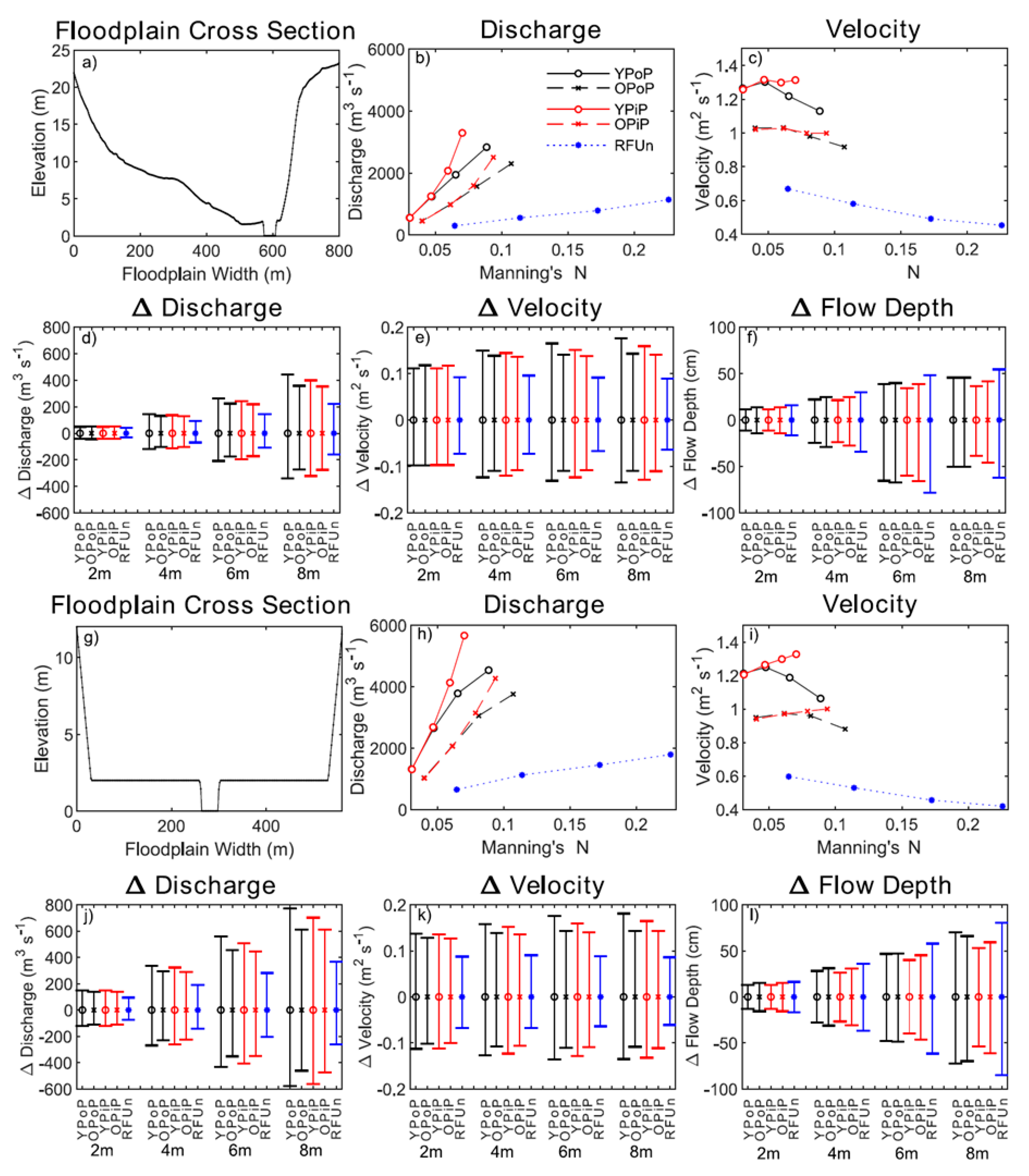
3.2.3. Demonstrating Flow Prediction and Incorporating Roughness Uncertainty

Uncertainty in remote sensing estimated forest structure is first propagated to roughness (as in Section 3.2.2 above), and then this study demonstrates how this uncertainty affects flow characteristics of discharge, velocity, and water depth over two test floodplain cross-sections. The two cross-sections presented in this study are directly upstream of Evesham on the river Avon, UK, with the topography defined from Environment Agency Lidar, and the other is a generic flat floodplain of 500 m cross-sectional width, similar in length to the Avon. The Evesham site was chosen as gauging station data and indicated a >5.5 m flow depth event during the 2007 summer floods (https://nrfa.ceh.ac.uk/data/station/peakflow/54002). The bankfull depth was taken to be 2 m, as stated in the Evesham gauging station. Discharge (Q) and depth-averaged velocity (Uc) are first calculated at 2, 4, 6, and 8 m flow depth using the standard Manning’s equation using a composite roughness value over the floodplain of each of the 5 floodplain forest types as a function of water depth. The composite floodplain roughness was based off Equations (6)–(18) from Reference [127], assuming that the total force resisting the flow in the cross-section is equal to the sum of forces resisting the flow in each cross-sectional perimeter bins. Where the floodplain is not flat, the Manning’s roughness applied to each topographical point changed to reflect the actual depth (e.g., flow depth next to the bank may be 2 m, but 100 m away from the bank may be 1 m). To illustrate the propagation of uncertainty, the 5 floodplain forest types were applied uniformly in space demonstrating full floodplain reforestation scenarios. In the Manning’s equation, the slope (S) was defined as 0.0005 from Lidar at Evesham and was considered constant at all discharge levels, and the cross-sectional area to flow (A) and hydraulic radius (R) were calculated based on the area wetted by the flow. With uneven topography, A is calculated as the integral between ground elevation and flow elevation at each discretized point along the floodplain cross-section. The wetted perimeter necessary for determining R is calculated as the sum of hypotenuse lengths of each discretized cross-section bin.
Uncertainty propagation through discharge and depth-averaged velocity was achieved by altering the Manning’s roughness value in the Manning’s equation for each of the 5 forest types. The amount Manning’s n is varied corresponds to combined mean literature uncertainty in remote sensing forest structure discussed in Section 2. In other words, the ± 20, 10, 30, 20% uncertainty in stem density, trunk diameter, wood area and leaf area indices is systematically propagated through Equations (1)–(3) first obtaining upper and lower roughness uncertainty estimates, which are then used to calculate upper and lower discharge and velocities for each forest type. Water Depth uncertainty is achieved by iteratively matching the left-hand side of the Manning’s equation below (Equation (4)) with the right-hand side, where water depth is changed in the right-hand side reflected in the cross-section area of flow A and hydraulic radius R:
( Q × n ) S = A × R 2 / 3   .

4. Results

4.1. Uncertainty in Roughness Estimates Resulting from Errors in Forest Structure Measurements

The size class distribution of each of the five forest types are presented in Figure 1 (top row), along with the vertical distribution LAI and WAI for each forest type (Figure 1, middle row). Using Equations (1)–(3), Manning’s n using the control forest structure is provided in Figure 1-bottom row. Remote sensing errors in estimating forest structural variables—stem density, DBH, WAI, and LAI—are propagated through the roughness Equations (1)–(3). Stem density and WAI are varied by 10–40%, and DBH and LAI are varied by 10–30%, according to Table 1 and Table 2. The resulting uncertainty of Manning’s n roughness up to 8 m flow depth due to errors in forest structural parameters is given in Figure 2.
Uncertainty in estimating stem density using remote sensing by 10, 20, 30, and 40% results in average changes in Manning’s n by 4.2, 8.4, 12.8, and 17.2%, respectively, at 2 m flow depth by 2.9, 5.9, 8.9, and 12%, respectively, at 8 m flow depth (Figure 2). This is an increase of Manning’s n uncertainty by 3–4.2% for every 10% uncertainty increase in stem density. Manning’s n estimates are most sensitive to uncertainties in stem density at the lowest flow depth of 2 m, with decreasing sensitivity for higher flow depths. This is true for the poplar plantations and especially for the unmanaged riparian forest (decrease in roughness sensitivity from 16.8–4.7% at 40% stem spacing uncertainty from 2–8 m flow depths). This is because the proportion of stem roughness, and so the influence of stem density, becomes smaller with an increase in woody and leaf roughness contribution. The unmanaged riparian forest has wood and leaf area starting from only a couple of meters from the ground (Figure 1). The pine plantations do not contain any leafy nor woody material within the first 8 m, resulting in equal sensitivity values throughout the vertical profile (Figure 2).
Uncertainty in estimating trunk diameter (DBH) using remote sensing by 10, 20, and 30% results in average changes in Manning’s n by 3.5, 7.0, 10.5%, respectively, at 2 m flow depth and 2.4, 4.9, 7.4%, respectively, at 8 m flow depth (Figure 2). This is an increase of Manning’s n uncertainty by 2.5–3.6% for every 10% uncertainty increase in DBH. As for stem spacing, the largest uncertainty in Manning’s n are a result of DBH uncertainty at the lowest flow depth of 2 m. As for stem spacing, this is due to the decreasing proportional influence of DBH with an increase in woody and leaf roughness contribution at higher flow depths.
Uncertainty in estimating WAI using remote sensing produces a different vertical change in Manning’s n (Figure 2). Here, WAI uncertainties by 10, 20, 30, and 40% results in average uncertainties in Manning’s n by 1.3, 2.6, 3.8, 5.1%, respectively, at 8 m flow depth with less than 0.15% for 2 m flow depths (these values include pine plantations). This is an increase of Manning’s n uncertainty at 8 m flow depths by 1.3% for every 10% uncertainty increase in DBH. Increases in roughness sensitivity with height are due to increasing woody areas for forest types with low canopies (see Figure 1, middle row). The unmanaged riparian site and the old poplar plantation increase in Manning’s n uncertainty to ~10% at 8 m flow depth at 40% WAI uncertainty. These two forest types have the highest WAI (WAI = 0.917–1.361) and so are expected to have the largest roughness sensitivity to changes in woody area.
Uncertainty in estimated LAI also results in increasing roughness uncertainty at deeper flows (Figure 2). LAI uncertainties of 10, 20, and 30% results in average uncertainty in Manning’s n by 0.9, 1.8, 2.7%, respectively, at 8 m flow depth with less than 0.25% for 2 m flow depths (averages include pine plantations). As with WAI, LAI for the poplar plantations and the unmanaged riparian forest started from within the first few meters. The unmanaged riparian site had a larger LAI than the old poplar plantation (5.306 vs 3.997) and a canopy that started within the first 2 m of tree height. This resulted in roughness being 3 times more sensitive to changes in LAI between the unmanaged riparian and the old poplar plantation.
Of the four forest structure variables, uncertainty in deriving stem density resulted in the largest uncertainty in Manning’s n, with Manning’s n varying by 4–4.5% at 2 m flow depths every 10% stem density uncertainty increase. Uncertainty in DBH was also substantial in varying Manning’s n by 3.1–3.9% at 2 m flow depths every 10% DBH uncertainty increase. Stem density and DBH uncertainty also result in the largest roughness sensitivity at 8 m flow depths, for 3 out of 5 forest sites, with Manning’s n varying by 1.2–4.5% every 10% stem density uncertainty increase and 1–3.9% every 10% DBH uncertainty increase. WAI and LAI uncertainty becomes important for increasing flow depths, with resulting uncertainty of Manning’s n at 8 m flow depth of up to 2.6 and 2.9% per 10% uncertainty increase in WAI and LAI. For the Young Poplar Plantation and the Unmanaged Riparian Forest, LAI uncertainty results in the largest roughness sensitivity at 8 m flow depths: 2.6 and 2.9%, respectively, for every 10% LAI uncertainty increase.
Yet, uncertainties in defining forest structure are not confined to one attribute. Uncertainties in all four forest structural variables are likely to be present if remote sensing is used to estimate roughness of a forested region. Figure 3a,b shows uncertainty of Manning’s n roughness to mean literature errors and maximum literature errors, respectively, in forest structural uncertainty. Using mean literature values in stem density, DBH, WAI, and LAI (i.e., 20, 10, 30, 20% uncertainty, respectively) results in combined uncertainty in Manning’s n from 11–13% to 11–17% at 2 m to 8 m flow depths. Using maximum literature errors in stem density, DBH, WAI and LAI (i.e., 40, 30, 40, 30% uncertainty, respectively) results in combined uncertainty in Manning’s n from 26–29% to 25–29% at 2 m to 8 m flow depths. Therefore, with combined uncertainties, the sensitivity of roughness estimates to errors in forest structure variables is around 7–8% for every 10% increase in combined forest structure uncertainty (see Table S1).
Propagating uncertainties in the species-specific drag coefficient (Cdi) and the species-specific deformation parameter (χi) up to 50% to roughness are provided in Figure S1. Uncertainties for these two parameters result in high sensitivities in roughness, with 3.8 and 5.5% sensitivity in Manning’s n for every 10% uncertainty increase in Cdi and χi, respectively.

4.2. Implications of Roughness Uncertainty on Flow

Figure 4 presents uncertainty in discharge, depth-averaged velocity, and flow depth propagated from the uncertainty in Manning’s n roughness from combined mean literature errors (see Figure 3a) in stem density, DBH, WAI, and LAI. The magnitude of discharge (Figure 4 panels b,h) and depth-averaged velocity (Figure 4 panels c,i) reflect the shape of the floodplains and the type of floodplain forest. Flow through the river Avon cross-section (Figure 4a) is calculated with discharge up to 550–1250 m3 s−1 at 4 m flow depth, which is 47–49% lower than flow through the generic floodplain (Figure 4g) calculating discharge up to 1100–2700 m3 s−1 at 4 m flow depth. At 8 m flow depth, the difference increases to 58–63% between floodplains. Note the gauging station on the Avon at Evesham estimated discharge at 3.5 m flood depth above bankfull level, to 464 m3 s−1 in July 2007. Depth-averaged velocities calculated from the river Avon cross-section are only around 4–10% higher than the generic floodplain at 4 m flow depth (0–8% at 8 m). In both floodplains, flow through the Unmanaged Riparian Forest resulted in the lowest discharge and velocity, and flow through the Young Pine Plantation had the highest discharge and velocity, reflecting their respective control roughness values (see Figure 1, bottom row).
The uncertainty in discharge, propagated from uncertainty in roughness, increases from around 10% to 12%, 13%, and 13.5 % at 2, 4, 6, and 8 m flow depths (~45, 115, 195, 315 m3 s−1) at the Avon river cross-section (Figure 4d). The uncertainty in discharge over the generic floodplain (Figure 4j) increased similarly from around 11.5% to 12.5%, 13.5%, and 14% at 2, 4, 6, and 8 m flow depths (~120, 255, 400, 540 m3 s−1). The smallest absolute uncertainties in discharge resulted from roughness uncertainties of the Unmanaged Riparian Forest, then the Old Pine and Poplar Plantations, and finally the Young Pine and Poplar Plantations (Figure 4d, j). The relative uncertainty is opposite, with the highest discharge uncertainty, for all flow depths at the river Avon cross-section, at 12–17% for Unmanaged Riparian Forest, 10.5–12.5% for Old Pine and 10.5–13.5% for Old Poplar Plantations, and 8–11% for Young Pine and 8–13.5% for Young Poplar Plantations (these relative uncertainties are on average 1% higher at the generic floodplain).
Interestingly, unlike discharge, absolute depth-averaged velocity uncertainties, propagated from uncertainty in roughness (Figure 4e,k) show very similar magnitudes, regardless of the tested floodplain, i.e., uncertainties of ~0.101, 0.120, 0.122, 0.125 m s−1 at 2, 4, 6, and 8 m flow depths at the river Avon cross-section versus uncertainties of ~0.111, 0.121, 0.125, 0.126 m s−1 at 2, 4, 6, and 8 m flow depths at the generic cross-section. The reason is that depth-averaged velocity is calculated as discharge per unit area (i.e., Q/A), taking away the influence of the floodplain shape. Similar to discharge, relative uncertainties in velocity are also similar between the floodplains tested, i.e., uncertainties of 10–13.5% and 11.5–14% at 2–8 m flow depths at the Avon and generic cross-sections, respectively. As with discharge uncertainty, the relative velocity uncertainties resulting from each floodplain forest type are the same as described in the previous paragraph.
Flow Depth is affected by the uncertainty in Manning’s roughness even at low to medium flow by decimeters (Figure 4f,l). With flow over the river Avon cross-section, uncertainty in roughness results in changes in flow depth from 2, 4, 6, and 8 m by 11–17 cm, 22–34 cm, 34–78 cm, and 36–62 cm, respectively (Figure 4f). The large range in flow depth changes with a 6 m floodplain depth are caused by the topography (see flattening out in Figure 4a). With flow over the generic floodplain, uncertainty in roughness also resulted in decimeter changes in flow depth from 2, 4, 6, and 8 m by 13–17 cm, 26–37 cm, 40–62 cm, and 53–85 cm, respectively (Figure 4l). In terms of forest type, roughness uncertainty over Unmanaged Riparian Forests, with leaves closer to the ground, had the largest effect on flow depth uncertainty, with a flow depth change from 2, 4, 6, and 8 m by around 16, 32, 63, and 58 cm, respectively. Flow depth uncertainty using Old and Young Pine Plantations was around 13, 25, 53, 48 cm, and using Old and Young Poplar Plantations was around 13, 24, 50, 41 cm for original depths of 2, 4, 6, and 8 m, respectively. Similar patterns exist with flow over the generic floodplain.

5. Discussion

Determining vegetation roughness of all aspects of a tree’s complex structure is crucial considering extreme flood frequency may increase with climate change for many parts of the world [1,2]. Quantifying blockage to flow in complex vegetative environments is an essential step to then modeling the effects of various reforestation scenarios upon flood mitigation. Vegetative blockage to flow can be parameterized using an appropriate roughness equation (see Equation (1)) and input data gathered using remote sensing technology, namely terrestrial and airborne lidar. This study has propagated the uncertainty in remote sensing derivations of complex woody vegetation structure—namely on defining stem density, trunk diameter, branch, and leaf areas—through roughness prediction for different forest types and for potentially extreme flows. This study then demonstrates the implications of roughness uncertainty on flow discharge, depth-averaged velocity, and flow depth using two test floodplain cross-sections.
Monitoring and measuring floodplain forests should ideally incorporate at least two remote sensing instruments—terrestrial and small-footprint airborne lidar—with campaigns in both winter and summer. Here, stem spacing using TLS, small footprint and large footprint lidar report similar uncertainties of up to 35% (Table 1). Trunk diameters should be monitored from TLS with multiple scans, with uncertainties of 4–20% (Table 1). Small-footprint lidar can estimate trunk diameters to similar levels of uncertainty (5–23%), although cannot readily detect smaller trunk diameters of understory trees. The vertical distribution of branches should be determined using TLS (Table 2). Yet, future work on scanning winter forests could determine vertical wood area indices using airborne lidar (e.g., Reference [84,101]). To determine leafy structure and LAI, small-footprint airborne lidar is best with uncertainties of around 6–30% (Table 2). In this case, TLS is worse that small and large-footprint lidar in detecting leafy structure, with uncertainty of up to 45%. If a single instrument is used for all four forest structure components, then TLS will produce the lowest uncertainty for all components except LAI, although LAI uncertainty offers the lowest change in Manning’s n uncertainty (see Figure 3). Using small-footprint airborne lidar only will improve leaf area estimations and maintain similar uncertainty for stem spacing and trunk diameter but may increase uncertainty for the branch components (see Table 2). An effective magnitude of this increase in uncertainty cannot be given due to the lack of ALS studies deriving branching structure.
Uncertainty in Manning’s n is smaller than any of the individual forest structure components (Figure 2 and Figure 3), with uncertainty in deriving stem density and DBH contributing the largest uncertainty to calculating Manning’s n (10% uncertainty in stem density and DBH resulted in ~4.2% and ~3.5% uncertainty in roughness, respectively). For more extreme flow entering the canopy, the uncertainty in defining WAI and LAI become more important, resulting in uncertainty to calculating Manning’s n by up to 2.6% and 2.9% per 10% uncertainty increase in WAI and LAI. For these reasons, improving remote sensing methods that estimate trunk diameter and stem spacing should be prioritized over canopy structure, in floodplains with a likelihood of low flood depths. For larger flood depths, TLS and airborne lidar should be used to reduce errors in estimating woody and leafy structure. Of course, this also depends on the type of forest (see next two paragraphs). Uncertainty in Manning’s n is also smaller than the combined forest structure components (Figure 3), where a 10% increase in combined forest structure uncertainty results in Manning’s n uncertainty of 7–8% (also, see Table S1).
River re-naturalization is currently being promoted by the UK-Government through Natural England and the Environment Agency to create an interconnected channel and floodplain system that serves both flood defense and biodiversity targets through the enhancement of natural processes. One approach is to develop and manage riparian and floodplain vegetation communities to increase roughness and decrease flood wave celerity. Evidence has shown that floodplain woodland can slow flood wave travel time and increase temporary flood storage (e.g., Reference [20]) and that older forest enhances this effect [128]. Modeling studies have also demonstrated the beneficial effects of floodplain forest in ‘slowing the flow’ [129,130]. However, most modeling studies simplify floodplain roughness often assuming uniform roughness across a given area, and often for a single species (e.g., Reference [131]). Catchment managers interested in restoring floodplain forest for flood risk management, require better information concerning the most appropriate species to plant, or to manage for. Catchment managers also need to understand how floodplain roughness will change over time, with tree growth and vegetation succession [131]. Better species-specific information will improve the predictive capabilities of the next generation of flood inundation models.
Our findings have floodplain management implications if floodplain reforestation or plantations are a desired NFM strategy for flood mitigation. First, as expected, forests with a higher basal area offer more resistance than sparser forests. Figure 1 shows that older and denser plantations offered 30% more resistance in the first 2 m flow depths than younger and sparser plantations. Roughness of older plantations are up to 5% more sensitive to uncertainty in stem density and DBH than young plantations but up to 4.6% and 1.8% less sensitive to uncertainty in WAI and LAI than young plantations (Figure 2). Therefore, deriving lower uncertainty stem density and DBH is more important for older forest plantations, while deriving lower uncertainty WAI and LAI is more important for younger plantations due to their lower canopies (Figure 1). Second, forests with lower canopies (e.g., the unmanaged riparian forest) offer more resistance than forests with higher canopies (e.g., old plantations), and uncertainties in WAI and LAI result in higher roughness uncertainties in lower than higher canopies. The unmanaged forest has higher LAI and WAI than the old plantations, resulting in (see Figure 1) up to 12% higher sensitivities to LAI and WAI uncertainties at 8 m flow depth (Figure 2). Third, poplar or other deciduous plantations have higher Manning’s n than pines, most notably when floodwater exceeds 6 m in flow depth (Figure 1 bottom panel). This is again due to woody and leafy area beginning lower in the canopy for poplars.
Uncertainty in defining forest structural variables have implications not only for roughness, but also for floodplain flow and flow depth, and ultimately on flow mitigation, as demonstrated in this study. Even with smaller floods, uncertainty in roughness can change flow depth by a decimeter, and, for larger deeper flows, flow depth can change by 40 cm or more (Figure 4). Floodplain topography in this context, can be important, especially in areas with a gentle slope, where a small change in flow depth is met with a larger frontal area of trees (compare Figure 4a, f). In terms of flow mitigation, unmanaged riparian forests offer the highest resistance to flow (Figure 1, bottom row), and so the lowest discharge and depth-averaged velocity, with the lowest absolute uncertainty in discharge and velocity (Figure 4) when propagating roughness uncertainty. Yet, incorrectly defining forest structural variables using remote sensing for this type of forest can result in the highest flow depth uncertainty of 32–63 cm from 4–6 m flow depths (5–16 cm more uncertainty than pine or poplar plantations). This cements the need for remote sensing methods to work on reducing uncertainty in defining dense riparian forest structure for stems, branches and leaves. This is especially important as much of the literature stated in Table 1 and Table 2 have not focused on complex-structure and multi-species forests. Old pine and poplar plantations offer more resistance to flow than young plantations (Figure 1), and so have lower discharge and depth-averaged velocity, and lower absolute uncertainty in discharge and velocity (Figure 4) when propagating roughness uncertainty. Yet, with extreme flow depths increasing to 6 m, uncertainty in roughness for the young poplar plantation, equals and surpasses the old pine plantation in flow depth uncertainty. This is due to low presence of branches and leaves, and the high uncertainty in WAI especially (30%; Figure 3a). Therefore, when considering which remote sensing technique to use and acceptable uncertainties in defining forest structure in flooding scenarios, it is necessary to consider the magnitude of desired flood event, the type of forest, and how low the canopy starts.
A source of error that has not been discussed in this study is that of determining forest types. Estimating forest types is needed to calculate local and reach-scale frontal area and friction factors (Equation (1)) for mixed-species forests. Forest composition errors may result in large roughness errors, based on 0–50% uncertainty propagation of the species-specific drag coefficient and deformation parameter shown in Figure S1. Current regional and global-scale ecosystem composition products are derived from multispectral remote sensing of broadly-defined land cover categories. These include products, such as the Moderate Resolution Imaging Spectroradiometer (MODIS) [132], distinguishing 5 broad global forest classes at up to 500 m, and the UK Center for Environment and Hydrology (CEH; Reference [133]), which distinguishes 10 vegetation types, including only 2 forest classes. In recent decades, higher spectral resolution imaging spectrometry has been used to provide meaningful plant classifications of both species and functional groups. Imaging spectroscopy has been shown to produce higher accuracies than multi-spectral sensors [134,135], and has been used to classify plant species or plant functional types in temperate forests (e.g., Reference [136,137,138]). In the past two decades, Multiple Endmember Spectral Mixture Analysis (MESMA) has been successfully applied for plant species classification [138,139,140]. MESMA uniquely estimates the fractional contribution of each pixel, i.e., resulting in multiple plant functional types per pixel. This technique is very useful in determining species abundance within a mixed forest plot. Architectural differences in forests could also be differentiated based on their vertical structure using lidar or multi-baseline interferometric radar (e.g., Reference [141,142,143]).
Certain riparian and floodplain tree species have not been investigated in this study, including Salix, Ulmus, Quercus, and Alnus. Salix and Alnus have low canopies, or canopies starting close to the ground, meaning they will behave similar to the Unmanaged Riparian Forest shown in this study, where better defining the trunk, stem density, and the canopy characteristics will all be important to reduce error propagation from remote sensing to roughness and flow depth estimations. For Quercus and Ulmus with larger trunks and high basal areas, correctly defining stem structure will be important in reducing roughness uncertainty. Future research should focus on expanding the effects of roughness and flow uncertainty through these important floodplain species, as well as investigating uncertainty propagation linked to natural forest patches of different ages and of different spatial distribution. Finally, active satellite imagery, such as GEDI (Global Ecosystem Dynamics Investigation) lidar or future BIOMASS radar, have not been described in this study, but could determine large scale forest structural attributes. Furthermore, SWOT (Surface Water and Ocean Topography) could be used to better determine water surface elevations, river widths, and dynamics slopes in calculating the effects of roughness uncertainty in flow discharge and depth.

6. Conclusions and Recommendations

NFM has advocated reforestation to improve ecological, sediment, and hydraulic connectivity of riverine landscapes whilst reducing flood risk. Yet, to adequately predict the effects of forests on medium-extreme magnitude floods, forests as resistance agents need to be appropriately parameterized in hydraulic models. Complex vegetation structure cannot easily be determined from field-based campaigns, while remote sensing offers high-resolution datasets capable of characterizing woody vegetation at larger spatial scales. This study, for the first time, has propagated the uncertainty in remote sensing derivations of complex vegetation structure first through roughness prediction and then through floodplain flow (discharge, velocity, and flow depth) for potentially extreme flows and different forest types (young and old Poplar plantations, young and old Pine plantations, and an unmanaged riparian forest). For the lowest uncertainty in forest structural variables, terrestrial laser scanning and small-footprint lidar should be used. Using mean literature remote sensing uncertainties in stem density, trunk diameter, WAI, and LAI (i.e., 20, 10, 30, 20% uncertainty, respectively) resulted in a combined uncertainty in Manning’s n from 11–13% to 11–17% at 2 m to 8 m flow depths. Individually, stem density and trunk diameter uncertainties resulted in the largest uncertainty in calculating Manning’s n at all flow depths, while, for extreme flows, leaf and woody area become more important. Even with smaller flows, these uncertainties in roughness can change flow depth by a decimeter, and, for larger flows, by 40 cm or more. These effects vary with forest type, where remote sensing errors in leaf and woody area are largest for low lying canopies, while errors in stem characteristics are largest in tall plantations with high basal areas. Therefore, this study highlights the need for lower uncertainty in all forest structure components using remote sensing, depending on forest type and flood magnitude, to improve roughness parameterization and flood modeling.
We present recommendations needed to advance the science behind vegetation roughness parameterization and remote sensing:
(A)
Uncertainty in deriving stem density results in the largest uncertainty in calculating Manning’s n. Remote sensing studies should focus on stem location and spacing uncertainty in dense stands of > 500 stems ha-1. DBH uncertainty is also important, and attention should be paid to deriving DBH from remote sensing with uncertainties below 10%.
(B)
Uncertainty in deriving WAI results in larger uncertainty in Manning’s n for deeper flows, yet remote sensing has not focused on determining woody area. Therefore, developing methods and using technology that can best determine vertical WAI is vital, from TLS to ALS campaigns.
(C)
Consequently, improving LAI (and WAI) estimations are much more important for forests with a low canopy, such as natural or semi-natural riparian forests. This becomes very important when considering the effect of remote sensing uncertainty in calculating LAI and WAI on flow depth for natural floodplain forests (Figure 4).
(D)
Roughness of extreme flow around tall trees needs to be calibrated. This would potentially create better flexibility parameters and drag coefficients, or inform us whether the current roughness equations are inadequate. Potential experiments could include monitoring floodwater during an actual large flood event within forest stands. Another solution may be to use laboratory flumes with microscale trees incorporating complex structure, and then extrapolate these results to the actual scale using appropriate scaling functions (see Reference [144] on multiscale numerical analyses).
(E)
Vertical roughness needs better parameterization in hydraulic models, beyond a single roughness value per horizontal grid-cell. One solution has been to simulate a flood event multiple times and iteratively change each grid-cell’s single-value roughness to match the flow depth (e.g., see Reference [145]). Remote sensing is capable of measuring vertical canopy structure and so have the ability to define vertical roughness (e.g., Reference [24]). The next step is to have this appropriate complexity represented in hydraulic models as stage-dependent roughness.

Supplementary Materials

The following are available online at https://www.mdpi.com/2072-4292/12/11/1799/s1, Document S1: Supplementary Roughness Equations- Vegetation Roughness of Trunks, Branches and Leaves, Figure S1: Sensitivity of Manning’s n roughness to error in the species-specific drag coefficient (Cdi) and the species-specific deformation parameter (χi) by 10, 20, 30, 40, and 50%. Sensitivity is tested over five forest types: Young and Old Poplar Plantations, Young and Old Pine Plantations, and an Unmanaged Riparian Forest, Table S1: Sensitivity of Manning’s n roughness to the combined errors of stem spacing, DBH, WAI, and LAI for the first 8 m in flow depth within canopies. This is where all structural parameters are varied by 10, 20, 30, and 40% in combination. Sensitivity is tested over five forest types: Young and Old Poplar Plantations, Young and Old Pine Plantations, and an Unmanaged Riparian Forest, and the control Manning’s n values before applying forest uncertainty is also presented.

Author Contributions

Conceptualization, A.S.A. and D.J.M.; Formal analysis, A.S.A.; Investigation, A.S.A. and D.J.M.; Methodology, A.S.A. and D.J.M.; Validation, A.S.A.; Visualization, A.S.A.; Writing – original draft, A.S.A. and D.J.M.; Writing – review & editing, A.S.A. and D.J.M. All authors have read and agreed to the published version of the manuscript.

Funding

This research received no external funding.

Acknowledgments

The authors would like to thank Julian Leyland, Daniel Parsons, and Stuart Lane for discussions at the conception of this paper. Furthermore, we thank the two anonymous reviewers for their constructive comments to this paper.

Conflicts of Interest

The authors declare no conflict of interest for this article.

References

  1. Brakenridge, G.R. Global Active Archive of Large Flood Events. In Dartmouth Flood Observatory; University of Colorado: Boulder, CO, USA, 2018; Available online: http://floodobservatory.colorado.edu/Archives/index.html (accessed on 16 February 2018).
  2. Hirabayashi, Y.; Mahendran, R.; Koirala, S.; Konoshima, L.; Yamazaki, D.; Watanabe, S.; Kim, H.; Kanae, S. Global flood risk under climate change. Nat. Clim. Chang. 2013, 3, 816–821. [Google Scholar] [CrossRef]
  3. Wheater, H.; Evans, E. Land use, water management and future flood risk. Land Use Policy 2009, 26, S251–S264. [Google Scholar] [CrossRef]
  4. Rogger, M.; Agnoletti, M.; Alaoui, A.; Bathurst, J.C.; Bodner, G.; Borga, M.; Chaplot, V.; Gallart, F.; Glatzel, G.; Hall, J.; et al. Land-use change impacts on floods at the catchment scale–Challenges and opportunities for future research. Water Resour. Res. 2017, 53, 5209–5219. [Google Scholar] [CrossRef] [Green Version]
  5. GWSP Digital Water Atlas. Map 51: Sediment Trapping by Large Dams (V1.0). 2008. Available online: https://water-future.org/gwsp-archive-digitalwateratlas/ (accessed on 1 April 2020).
  6. Syvitski, J.P.; Vörösmarty, C.J.; Kettner, A.J.; Green, P. Impact of humans on the flux of terrestrial sediment to the global coastal ocean. Science 2005, 308, 376–380. [Google Scholar] [CrossRef]
  7. Brooker, M.P. The ecological effects of channelization. Geogr. J. 1985, 151, 63–69. [Google Scholar] [CrossRef]
  8. Oscoz, J.; Leunda, P.M.; Miranda, R.; García-Fresca, C.; Campos, F.; Escala, M.C. River channelization effects on fish population structure in the Larraun river (Northern Spain). Hydrobiologia 2005, 543, 191–198. [Google Scholar] [CrossRef]
  9. Castello, L.; McGrath, D.G.; Hess, L.L.; Coe, M.T.; Lefebvre, P.A.; Petry, P.; Macedo, M.N.; Reno, V.; Arantes, C.C. The vulnerability of Amazon freshwater ecosystems. Conserv. Lett. 2012, 6, 217–229. [Google Scholar] [CrossRef]
  10. Van den Honert, R.C.; McAneney, J. The 2011 Brisbane floods: Causes, impacts and implications. Water 2011, 3, 1149–1173. [Google Scholar] [CrossRef] [Green Version]
  11. Monbiot, G. Dredging rivers won’t stop floods. It will make them worse. The Guardian. 30 January 2014. Available online: https://www.theguardian.com/commentisfree/2014/jan/30/dredging-rivers-floods-somerset-levels-david-cameron-farmers (accessed on 1 April 2020).
  12. Wentworth, J. Natural Flood Management; The UK Parliamentary Office of Science and Technology notes, POST-PN-396; Parliamentary Office of Science and Technology: London, UK, 2011. [Google Scholar]
  13. Wharton, G.; Gilvear, D.J. River restoration in the UK: Meeting the dual needs of the European Union Water Framework Directive and flood defence? Int. J. River Basin Manag. 2007, 5, 143–154. [Google Scholar] [CrossRef]
  14. Nisbet, T.; Silgram, M.; Shah, N.; Morrow, K.; Broadmeadow, S. Woodland for water: Woodland measures for meeting Water Framework Directive objectives. In Forest Research Monograph: 4; Forestry Commission: Edinburgh, UK, 2011; p. 156. Available online: http://www.forestry.gov.uk/pdf/FRMG004_Woodland4Water.pdf/$FILE/FRMG004_Woodland4Water.pdf (accessed on 4 December 2017).
  15. Forestry Commission. Forests and Water. UK Forestry Standard Guidelines; Forestry Commission: Edinburgh, UK, 2011. [Google Scholar]
  16. CONFOR. Forestry and Flooding; Confederation of Forest Industries: Edinburgh, UK, 2016; Available online: http://www.confor.org.uk/media/246067/confor-37_forestryandfloodingreportfeb2016.pdf (accessed on 1 April 2020).
  17. Alila, Y.; Kuraś, P.K.; Schnorbus, M.; Hudson, R. Forests and floods: A new paradigm sheds light on age-old controversies. Water Resour. Res. 2009, 45, W08416. [Google Scholar] [CrossRef]
  18. FAO & CIFOR. Forests and Floods: Drowning in Fiction or Thriving on Facts? FAO Regional Office for Asia and the Pacific (RAP) Publication: Bangkok, Thailand, 2005. [Google Scholar]
  19. Calder, I.; Hofer, T.; Vermont, S.; Warren, P. Towards a new understanding of forests and water. Unasylva 2007, 58, 3–10. [Google Scholar]
  20. Thomas, H.; Nisbet, T.R. An assessment of the impact of floodplain woodland on flood flows. Water Environ. J. 2007, 21, 114–126. [Google Scholar] [CrossRef]
  21. Kouwen, N.; Unny, T.E. Flexible roughness in open channels. J. Hydraul. Division 1973, 99, 713–728. [Google Scholar]
  22. Järvelä, J. Determination of flow resistance caused by non-submerged woody vegetation. International J. River Basin Manag. 2004, 2, 61–70. [Google Scholar] [CrossRef]
  23. Antonarakis, A.S.; Richards, K.S.; Brasington, J.; Bithell, M. Leafless roughness of complex tree morphology using terrestrial lidar. Water Resour. Res. 2009, 45, W10401. [Google Scholar] [CrossRef] [Green Version]
  24. Antonarakis, A.S.; Richards, K.S.; Brasington, J.; Muller, E. Determining leaf area index and leafy tree roughness using terrestrial laser scanning. Water Resour. Res. 2010, 46, W06410. [Google Scholar] [CrossRef] [Green Version]
  25. Tanino, Y.; Nepf, H.M. Laboratory investigation of mean drag in a random array of rigid, emergent cylinders. J. Hydraul. Eng. 2008, 134, 34–41. [Google Scholar] [CrossRef]
  26. Schoneboom, T.; Aberle, J.; Dittrich, A. Spatial variability, mean drag forces, and drag coefficients in an array of rigid cylinders. In Experimental Methods in Hydraulic Research; Springer: Berlin/Heidelberg, Germany, 2011; pp. 255–265. [Google Scholar]
  27. Baptist, M.; Babovic, V.; Uthurburu, J.R.; Keijzer, M.; Uittenbogaard, R.; Mynett, A.; Verwey, A. On inducing equations for vegetation resistance. J. Hydraul. Res. 2007, 45, 435–450. [Google Scholar] [CrossRef]
  28. Van Oorschot, M.; Kleinhans, M.; Geerling, G.; Middelkoop, H. Distinct patterns of interaction between vegetation and morphodynamics. Earth Surf. Process. Landf. 2016, 41, 791–808. [Google Scholar] [CrossRef]
  29. Solari, L.; Van Oorschot, M.; Belletti, B.; Hendriks, D.; Rinaldi, M.; Vargas-Luna, A. Advances on modeling riparian vegetation—Hydromorphology interactions. River Res. Appl. 2016, 32, 164–178. [Google Scholar] [CrossRef]
  30. Boothroyd, R.J.; Hardy, R.J.; Warburton, J.; Marjoribanks, T.I. The importance of accurately representing submerged vegetation morphology in the numerical prediction of complex river flow. Earth Surf. Process. Landf. 2016, 41, 567–576. [Google Scholar] [CrossRef] [Green Version]
  31. Aberle, J.; Järvelä, J. Flow resistance of emergent rigid and flexible floodplain vegetation. J. Hydraul. Res. 2013, 51, 33–45. [Google Scholar] [CrossRef]
  32. Västilä, K.; Järvelä, J. Characterizing natural riparian vegetation for modeling of flow and suspended sediment transport. J. Soils Sediments 2017, 18, 3114–3130. [Google Scholar] [CrossRef] [Green Version]
  33. Peterken, G.F.; Hughes, F.M.R. Restoration of floodplain forests in Britain. For. Int. J. For. Res. 1995, 68, 187–202. [Google Scholar] [CrossRef]
  34. Hughes, F.M.; del Tánago, M.G.; Mountford, J.O. Restoring floodplain forests in Europe. In A Goal-Oriented Approach to Forest Landscape Restoration; Springer: Dordrecht, The Netherlands, 2012; pp. 393–422. [Google Scholar]
  35. Forestry Commission Scotland. Seed sources for planting native trees and shrubs in Scotland. 2006. Available online: www.forestresearch.gov.uk/documents/7060/FCFC151.pdf (accessed on 1 April 2020).
  36. Liang, X.; Kankare, V.; Hyyppä, J.; Wang, Y.; Kukko, A.; Haggrén, H.; Yu, X.; Kaartinen, H.; Jaakkola, A.; Guan, F.; et al. Terrestrial laser scanning in forest inventories. ISPRS J. Photogramm. Remote Sens. 2016, 115, 63–77. [Google Scholar] [CrossRef]
  37. Kankare, V.; Liang, X.; Vastaranta, M.; Yu, X.; Holopainen, M.; Hyyppä, J. Diameter distribution estimation with laser scanning based multisource single tree inventory. ISPRS J. Photogramm. Remote Sens. 2015, 108, 61–171. [Google Scholar] [CrossRef]
  38. Maas, H.G.; Bienert, A.; Scheller, S.; Keane, E. Automatic forest inventory parameter determination from terrestrial laser scanner data. Int. J. Remote Sens. 2008, 29, 1579–1593. [Google Scholar] [CrossRef]
  39. Antonarakis, A.S. Evaluating forest biometrics obtained from ground lidar in complex riparian forests. Remote Sens. Lett. 2011, 2, 61–70. [Google Scholar] [CrossRef]
  40. Brolly, G.; Király, G. Algorithms for stem mapping by means of terrestrial laser scanning. Acta Silv. Et Lignaria Hung. 2009, 5, 119–130. [Google Scholar]
  41. Olofsson, K.; Holmgren, J.; Olsson, H. Tree stem and height measurements using terrestrial laser scanning and the RANSAC algorithm. Remote Sens. 2014, 6, 4323–4344. [Google Scholar] [CrossRef] [Green Version]
  42. Liang, X.; Hyyppä, J. Automatic stem mapping by merging several terrestrial laser scans at the feature and decision levels. Sensors 2013, 13, 1614–1634. [Google Scholar] [CrossRef] [PubMed] [Green Version]
  43. Calders, K.; Newnham, G.; Burt, A.; Murphy, S.; Raumonen, P.; Herold, M.; Culvenor, D.; Avitabile, V.; Disney, M.; Armston, J.; et al. Nondestructive estimates of above-ground biomass using terrestrial laser scanning. Methods Ecol. Evol. 2015, 6, 198–208. [Google Scholar] [CrossRef]
  44. Pouliot, D.A.; King, D.J.; Bell, F.W.; Pitt, D.G. Automated tree crown detection and delineation in high-resolution digital camera imagery of coniferous forest regeneration. Remote Sens. Environ. 2002, 82, 322–334. [Google Scholar] [CrossRef]
  45. Culvenor, D.S. TIDA: An algorithm for the delineation of tree crowns in high spatial resolution remotely sensed imagery. Comput. Geosci. 2002, 28, 33–44. [Google Scholar] [CrossRef]
  46. Ke, Y.; Quackenbush, L.J. A review of methods for automatic individual tree-crown detection and delineation from passive remote sensing. Int. J. Remote Sens. 2011, 32, 4725–4747. [Google Scholar] [CrossRef]
  47. Hyyppä, J.; Hyyppä, H.; Leckie, D.; Gougeon, F.; Yu, X.; Maltamo, M. Review of methods of small-footprint airborne laser scanning for extracting forest inventory data in boreal forests. Int. J. Remote Sens. 2008, 29, 1339–1366. [Google Scholar] [CrossRef]
  48. Huang, S.; Hager, S.A.; Halligan, K.Q.; Fairweather, I.S.; Swanson, A.K.; Crabtree, R.L. A comparison of individual tree and forest plot height derived from lidar and InSAR. Photogramm. Eng. Remote Sens. 2009, 75, 159–167. [Google Scholar] [CrossRef]
  49. Kathuria, A.; Turner, R.; Stone, C.; Duque-Lazo, J.; West, R. Development of an automated individual tree detection model using point cloud LiDAR data for accurate tree counts in a Pinus radiata plantation. Aust. For. 2016, 79, 126–136. [Google Scholar] [CrossRef]
  50. Antonarakis, A.S.; Richards, K.S.; Brasington, J.; Bithell, M.; Muller, E. Retrieval of vegetative fluid resistance terms for rigid stems using airborne lidar. J. Geophys. Res. Biogeosciences 2008, 113, G02S07. [Google Scholar] [CrossRef] [Green Version]
  51. Antonarakis, A.S.; Munger, J.W.; Moorcroft, P.R. Imaging spectroscopy-and lidar-derived estimates of canopy composition and structure to improve predictions of forest carbon fluxes and ecosystem dynamics. Geophys. Res. Lett. 2014, 41, 2535–2542. [Google Scholar] [CrossRef]
  52. Wallace, L.; Lucieer, A.; Watson, C.S. Evaluating tree detection and segmentation routines on very high resolution UAV LiDAR data. IEEE Trans. Geosci. Remote Sens. 2014, 52, 7619–7628. [Google Scholar] [CrossRef]
  53. Korpela, I. Individual tree measurements by means of digital aerial photogrammetry. Silva Fenn. Monogr. 2004, 3, 93. [Google Scholar]
  54. Ferraz, A.; Saatchi, S.; Mallet, C.; Meyer, V. Lidar detection of individual tree size in tropical forests. Remote Sens. Environ. 2016, 183, 318–333. [Google Scholar] [CrossRef]
  55. Persson, A.; Holmgren, J.; Soderman, U. Detecting and measuring individual trees using an airborne laser scanner. Photogramm. Eng. Remote Sens. 2002, 68, 925–932. [Google Scholar]
  56. Popescu, S.C. Estimating biomass of individual pine trees using airborne lidar. Biomass Bioenergy 2007, 31, 646–655. [Google Scholar] [CrossRef]
  57. Yu, X.; Hyyppä, J.; Vastaranta, M.; Holopainen, M.; Viitala, R. Predicting individual tree attributes from airborne laser point clouds based on the random forests technique. ISPRS J. Photogramm. Remote Sens. 2011, 66, 28–37. [Google Scholar] [CrossRef]
  58. Yao, W.; Krzystek, P.; Heurich, M. Tree species classification and estimation of stem volume and DBH based on single tree extraction by exploiting airborne full-waveform LiDAR data. Remote Sens. Environ. 2012, 123, 368–380. [Google Scholar] [CrossRef]
  59. Lefsky, M.A.; Harding, D.; Cohen, W.B.; Parker, G.; Shugart, H.H. Surface lidar remote sensing of basal area and biomass in deciduous forests of eastern Maryland, USA. Remote Sens. Environ. 1999, 67, 83–98. [Google Scholar] [CrossRef]
  60. Means, J.E.; Acker, S.A.; Fitt, B.J.; Renslow, M.; Emerson, L.; Hendrix, C.J. Predicting forest stand characteristics with airborne scanning lidar. Photogramm. Eng. Remote Sens. 2000, 66, 1367–1372. [Google Scholar]
  61. Drake, J.B.; Dubayah, R.O.; Clark, D.B.; Knox, R.G.; Blair, J.B.; Hofton, M.A.; Chazdon, R.L.; Weishampel, J.F.; Prince, S. Estimation of tropical forest structural characteristics using large-footprint lidar. Remote Sens. Environ. 2002, 79, 305–319. [Google Scholar] [CrossRef]
  62. Asner, G.P.; Mascaro, J.; Muller-Landau, H.C.; Vieilledent, G.; Vaudry, R.; Rasamoelina, M.; Hall, J.S.; Van Breugel, M. A universal airborne LiDAR approach for tropical forest carbon mapping. Oecologia 2012, 168, 1147–1160. [Google Scholar] [CrossRef] [PubMed]
  63. Yu, X.; Hyyppä, J.; Karjalainen, M.; Nurminen, K.; Karila, K.; Vastaranta, M.; Kankare, V.; Kaartinen, H.; Holopainen, M.; Honkavaara, E.; et al. Comparison of laser and stereo optical, SAR and InSAR point clouds from air-and space-borne sources in the retrieval of forest inventory attributes. Remote Sens. 2015, 7, 15933–15954. [Google Scholar] [CrossRef] [Green Version]
  64. Antonarakis, A.S.; Guizar-Coutiño, A. Regional carbon predictions in a temperate forest using satellite lidar. IEEE J. Sel. Top. Appl. Earth Obs. Remote Sens. 2017, 10, 4954–4960. [Google Scholar] [CrossRef] [Green Version]
  65. Fritz, A.; Kattenborn, T.; Koch, B. UAV-based photogrammetric point clouds—Tree stem mapping in open stands in comparison to terrestrial laser scanner point clouds. Int. Arch. Photogramm. Remote Sens. Spat. Inf. Sci. 2013, 40, 141–146. [Google Scholar] [CrossRef] [Green Version]
  66. Malhi, Y.; Jackson, T.; Bentley, L.P.; Lau, A.; Shenkin, A.; Herold, M.; Calders, K.; Bartholomeus, H.; Disney, M.I. New perspectives on the ecology of tree structure and tree communities through terrestrial laser scanning. Interface Focus 2018, 8, 20170052. [Google Scholar] [CrossRef] [PubMed] [Green Version]
  67. Gorte, B.; Pfeifer, N. Structuring laser-scanned trees using 3D mathematical morphology. Int. Arch. Photogramm. Remote Sens. 2004, 35, 929–933. [Google Scholar]
  68. Hosoi, F.; Omasa, K. Voxel-based 3-D modeling of individual trees for estimating leaf area density using high-resolution portable scanning lidar. IEEE Trans. Geosci. Remote Sens. 2006, 44, 3610–3618. [Google Scholar] [CrossRef]
  69. Widlowski, J.L.; Côté, J.F.; Béland, M. Abstract tree crowns in 3D radiative transfer models: Impact on simulated open-canopy reflectances. Remote Sens. Environ. 2014, 142, 155–175. [Google Scholar] [CrossRef]
  70. Raumonen, P.; Kaasalainen, M.; Åkerblom, M.; Kaasalainen, S.; Kaartinen, H.; Vastaranta, M.; Holopainen, M.; Disney, M.; Lewis, P. Fast automatic precision tree models from terrestrial laser scanner data. Remote Sens. 2013, 5, 491–520. [Google Scholar] [CrossRef] [Green Version]
  71. Douglas, E.S.; Martel, J.; Li, Z.; Howe, G.; Hewawasam, K.; Marshall, R.A.; Schaaf, C.L.; Cook, T.A.; Newnham, G.J.; Strahler, A.; et al. Finding leaves in the forest: The dual-wavelength Echidna lidar. IEEE Geosci. Remote Sens. Lett. 2015, 12, 776–780. [Google Scholar] [CrossRef]
  72. Ma, L.; Zheng, G.; Eitel, J.U.; Magney, T.S.; Moskal, L.M. Determining woody-to-total area ratio using terrestrial laser scanning (TLS). Agric. For. Meteorol. 2016, 228, 217–228. [Google Scholar] [CrossRef] [Green Version]
  73. Pueschel, P.; Newnham, G.; Rock, G.; Udelhoven, T.; Werner, W.; Hill, J. The influence of scan mode and circle fitting on tree stem detection, stem diameter and volume extraction from terrestrial laser scans. ISPRS J. Photogramm. Remote. Sens. 2013, 77, 44–56. [Google Scholar] [CrossRef]
  74. Dassot, M.; Colin, A.; Santenoise, P.; Fournier, M.; Constant, T. Terrestrial laser scanning for measuring the solid wood volume, including branches, of adult standing trees in the forest environment. Comput. Electron. Agric. 2012, 89, 86–93. [Google Scholar] [CrossRef]
  75. De Tanago, J.G.; Lau, A.; Bartholomeus, H.; Herold, M.; Avitabile, V.; Raumonen, P.; Martius, C.; Goodman, R.C.; Disney, M.; Manuri, S.; et al. Estimation of above-ground biomass of large tropical trees with terrestrial LiDAR. Methods Ecol. Evol. 2018, 9, 223–234. [Google Scholar] [CrossRef] [Green Version]
  76. Kankare, V.; Holopainen, M.; Vastaranta, M.; Puttonen, E.; Yu, X.; Hyyppä, J.; Vaaja, M.; Hyyppä, H.; Alho, P. Individual tree biomass estimation using terrestrial laser scanning. ISPRS J. Photogramm. Remote Sens. 2013, 75, 64–75. [Google Scholar] [CrossRef]
  77. Hauglin, M.; Astrup, R.; Gobakken, T.; Næsset, E. Estimating single-tree branch biomass of Norway spruce with terrestrial laser scanning using voxel-based and crown dimension features. Scand. J. For. Res. 2013, 28, 456–469. [Google Scholar] [CrossRef]
  78. MacArthur, R.H.; Horn, H.S. Foliage profile by vertical measurements. Ecology 1969, 50, 802–804. [Google Scholar] [CrossRef] [Green Version]
  79. Danson, F.M.; Hetherington, D.; Morsdorf, F.; Koetz, B.; Allgower, B. Forest canopy gap fraction from terrestrial laser scanning. IEEE Geosci. Remote Sens. Lett. 2007, 4, 157–160. [Google Scholar] [CrossRef] [Green Version]
  80. Jupp, D.L.; Culvenor, D.S.; Lovell, J.L.; Newnham, G.J.; Strahler, A.H.; Woodcock, C.E. Estimating forest LAI profiles and structural parameters using a ground-based laser called ‘Echidna®. Tree Physiol. 2009, 29, 171–181. [Google Scholar] [CrossRef]
  81. Strahler, A.H.; Jupp, D.L.; Woodcock, C.E.; Schaaf, C.B.; Yao, T.; Zhao, F.; Yang, X.; Lovell, J.; Culvenor, D.; Newnham, G.; et al. Retrieval of forest structural parameters using a ground-based lidar instrument (Echidna®). Can. J. Remote Sens. 2008, 34, S426–S440. [Google Scholar] [CrossRef] [Green Version]
  82. Hopkinson, C.; Lovell, J.; Chasmer, L.; Jupp, D.; Kljun, N.; van Gorsel, E. Integrating terrestrial and airborne lidar to calibrate a 3D canopy model of effective leaf area index. Remote Sens. Environ. 2013, 136, 301–314. [Google Scholar] [CrossRef]
  83. Zheng, G.; Ma, L.; He, W.; Eitel, J.U.; Moskal, L.M.; Zhang, Z. Assessing the contribution of woody materials to forest angular gap fraction and effective leaf area index using terrestrial laser scanning data. IEEE Trans. Geosci. Remote Sens. 2016, 54, 1475–1487. [Google Scholar] [CrossRef]
  84. Zhu, X.; Skidmore, A.K.; Wang, T.; Liu, J.; Darvishzadeh, R.; Shi, Y.; Premier, J.; Heurich, M. Improving leaf area index (LAI) estimation by correcting for clumping and woody effects using terrestrial laser scanning. Agric. For. Meteorol. 2018, 263, 276–286. [Google Scholar] [CrossRef]
  85. Morsdorf, F.; Kötz, B.; Meier, E.; Itten, K.I.; Allgöwer, B. Estimation of LAI and fractional cover from small footprint airborne laser scanning data based on gap fraction. Remote Sens. Environ. 2006, 104, 50–61. [Google Scholar] [CrossRef]
  86. Solberg, S.; Næsset, E.; Hanssen, K.H.; Christiansen, E. Mapping defoliation during a severe insect attack on Scots pine using airborne laser scanning. Remote Sens. Environ. 2006, 102, 364–376. [Google Scholar] [CrossRef]
  87. Barilotti, A.; Turco, S.; Alberti, G. LAI determination in forestry ecosystem by LiDAR data analysis. In Proceedings of the International Workshop 3D Remote Sensing in Forestry, Vienna, Austria, 14–15 February 2006; pp. 248–252. [Google Scholar]
  88. Jensen, J.L.; Humes, K.S.; Vierling, L.A.; Hudak, A.T. Discrete return lidar-based prediction of leaf area index in two conifer forests. Remote Sens. Environ. 2008, 112, 3947–3957. [Google Scholar] [CrossRef] [Green Version]
  89. Korhonen, L.; Korpela, I.; Heiskanen, J.; Maltamo, M. Airborne discrete-return LIDAR data in the estimation of vertical canopy cover, angular canopy closure and leaf area index. Remote Sens. Environ. 2011, 115, 1065–1080. [Google Scholar] [CrossRef]
  90. Hayduk, E.A. Using LiDAR Data to Estimate Effective Leaf Area Index, Determine Biometrics and Visualize Canopy Structure in a Central Oregon Forest with Complex Terrain. Ph.D. Thesis, Evergreen State College, Olympia, WA, USA, 2012. [Google Scholar]
  91. You, H.; Wang, T.; Skidmore, A.; Xing, Y. Quantifying the effects of normalisation of airborne LiDAR intensity on coniferous forest leaf area index estimations. Remote Sens. 2017, 9, 163. [Google Scholar] [CrossRef] [Green Version]
  92. Qu, Y.; Shaker, A.; Silva, C.; Klauberg, C.; Pinagé, E. Remote Sensing of Leaf Area Index from LiDAR Height Percentile Metrics and Comparison with MODIS Product in a Selectively Logged Tropical Forest Area in Eastern Amazonia. Remote Sens. 2018, 10, 970. [Google Scholar] [CrossRef] [Green Version]
  93. Ni-Meister, W.; Jupp, D.L.; Dubayah, R. Modeling lidar waveforms in heterogeneous and discrete canopies. IEEE Trans. Geosci. Remote Sens. 2001, 39, 1943–1958. [Google Scholar] [CrossRef] [Green Version]
  94. Ni-Meister, W.; Yang, W.; Kiang, N.Y. A clumped-foliage canopy radiative transfer model for a global dynamic terrestrial ecosystem model. I: Theory. Agric. Forest Meteorol. 2010, 150, 881–894. [Google Scholar] [CrossRef]
  95. Tang, H.; Dubayah, R.; Swatantran, A.; Hofton, M.; Sheldon, S.; Clark, D.B.; Blair, B. Retrieval of vertical LAI profiles over tropical rain forests using waveform lidar at La Selva, Costa Rica. Remote Sens. Environ. 2012, 124, 242–250. [Google Scholar] [CrossRef]
  96. Treuhaft, R.N.; Asner, G.P.; Law, B.E.; Van Tuyl, S. Forest leaf area density profiles from the quantitative fusion of radar and hyperspectral data. J. Geophys. Res. Atmos. 2002, 107, ACL 7. [Google Scholar] [CrossRef]
  97. Treuhaft, R.N.; Law, B.E.; Asner, G.P. Forest attributes from radar interferometric structure and its fusion with optical remote sensing. Aibs Bull. 2004, 54, 561–571. [Google Scholar] [CrossRef] [Green Version]
  98. Peduzzi, A.; Wynne, R.H.; Thomas, V.A.; Nelson, R.F.; Reis, J.J.; Sanford, M. Combined use of airborne lidar and DBInSAR data to estimate LAI in temperate mixed forests. Remote Sens. 2012, 4, 1758–1780. [Google Scholar] [CrossRef] [Green Version]
  99. Liang, X.; Kankare, V.; Yu, X.; Hyyppä, J.; Holopainen, M. Automated stem curve measurement using terrestrial laser scanning. IEEE Trans. Geosci. Remote Sens. 2014, 52, 1739–1748. [Google Scholar] [CrossRef]
  100. Hosoi, F.; Nakai, Y.; Omasa, K. 3-D voxel-based solid modeling of a broad-leaved tree for accurate volume estimation using portable scanning lidar. ISPRS J. Photogramm. Remote Sens. 2013, 82, 41–48. [Google Scholar] [CrossRef]
  101. Villikka, M.; Packalén, P.; Maltamo, M. The suitability of leaf-off airborne laser scanning data in an area-based forest inventory of coniferous and deciduous trees. Silva Fenn. 2012, 46, 99–110. [Google Scholar] [CrossRef] [Green Version]
  102. Tang, H.; Brolly, M.; Zhao, F.; Strahler, A.H.; Schaaf, C.L.; Ganguly, S.; Zhang, G.; Dubayah, R. Deriving and validating Leaf Area Index (LAI) at multiple spatial scales through lidar remote sensing: A case study in Sierra National Forest, CA. Remote Sens. Environ. 2014, 143, 131–141. [Google Scholar] [CrossRef]
  103. Manninen, T.; Stenberg, P.; Rautiainen, M.; Voipio, P.; Smolander, H. Leaf area index estimation of boreal forest using ENVISAT ASAR. IEEE Trans. Geosci. Remote Sens. 2005, 43, 2627–2635. [Google Scholar] [CrossRef]
  104. Stankevich, S.A.; Kozlova, A.A.; Piestova, I.O.; Lubskyi, M.S. Leaf area index estimation of forest using sentinel-1 C-band SAR data. In Proceedings of the 2017 IEEE Microwaves, Radar and Remote Sensing Symposium (MRRS), Kiev, Ukraine, 29–31 August 2017; pp. 253–256. [Google Scholar]
  105. Fathi-Moghadam, M.; Kouwen, N. Nonrigid, nonsubmerged, vegetative roughness on floodplains. J. Hydraul. Eng. 1997, 123, 51–57. [Google Scholar] [CrossRef]
  106. Mason, D.C.; Cobby, D.M.; Horritt, M.S.; Bates, P.D. Floodplain friction parameterization in two-dimensional river flood models using vegetation heights derived from airborne scanning laser altimetry. Hydrol. Process. 2003, 17, 1711–1732. [Google Scholar] [CrossRef]
  107. Lindner, K. Der Strömungswiderstand von Pflanzenbeständen. Ph.D. Thesis, Mitteilungen 75, Leichtweiss-Institut für Wasserbau, TU Braunschweig, Braunschweig, Germany, 1982. [Google Scholar]
  108. Archaux, F.; Martin, H. Hybrid poplar plantations in a floodplain have balanced impacts on farmland and woodland birds. Forest Ecol. Manag. 2009, 257, 1474–1479. [Google Scholar] [CrossRef] [Green Version]
  109. FAO. Poplars and Other Fast-Growing Trees - Renewable Resources for Future Green Economies. Synthesis of Country Progress Reports. In Proceedings of the 25th Session of the International Poplar Commission, Berlin, Germany, 13–16 September 2016; Working Paper IPC/15. Forestry Policy and Resources Division, FAO: Rome, Italy, 2016. Available online: http://www.fao.org/forestry/ipc2016/en/ (accessed on 1 April 2020).
  110. Ball, J.; Carle, J.; Del Lungo, A. Contribution of poplars and willows to sustainable forestry and rural development. UNASYLVA-FAO 2005, 56, 3. [Google Scholar]
  111. Mason, W.L.; Alía, R. Current and future status of Scots pine (Pinus sylvestris L.) forests in Europe. Forest Syst. 2000, 9, 317–335. [Google Scholar]
  112. Forestry Commission. Forestry Statistics 2018; Forestry Commission: Edinburgh, UK, 2018. [Google Scholar]
  113. Forestry Commission. North Tummel Land Management Plan; Forestry Commission: Edinburgh, UK, 2018; Available online: https://forestryandland.gov.scot/images/corporate/design-plans/tay/north-tummel/Draft_North_Tummel_LMP_summary.pdf (accessed on 1 May 2020).
  114. Robeson, D. River Floodplains and Natural Flood Management in Farmed Land; Technical Note TN646; The Scottish Agricultural College: Perth, UK, 2012. [Google Scholar]
  115. Heym, M.; Ruíz-Peinado, R.; Del Río, M.; Bielak, K.; Forrester, D.I.; Dirnberger, G.; Barbeito, I.; Brazaitis, G.; Ruškytkė, I.; Coll, L.; et al. EuMIXFOR empirical forest mensuration and ring width data from pure and mixed stands of Scots pine (Pinus sylvestris L.) and European beech (Fagus sylvatica L.) through Europe. Ann. For. Sci. 2017, 74, 63. [Google Scholar] [CrossRef] [Green Version]
  116. Price, C.A.; Enquist, B.J.; Savage, V.M. A general model for allometric covariation in botanical form and function. Proc. Natl. Acad. Sci. 2007, 104, 13204–13209. [Google Scholar] [CrossRef] [Green Version]
  117. Smith, D.D.; Sperry, J.S.; Enquist, B.J.; Savage, V.M.; McCulloh, K.A.; Bentley, L.P. Deviation from symmetrically self-similar branching in trees predicts altered hydraulics, mechanics, light interception and metabolic scaling. New Phytol. 2014, 201, 217–229. [Google Scholar] [CrossRef]
  118. Muukkonen, P. Generalized allometric volume and biomass equations for some tree species in Europe. Eur. J. For. Res. 2007, 126, 157–166. [Google Scholar] [CrossRef]
  119. Medvigy, D.; Wofsy, S.C.; Munger, J.W.; Hollinger, D.Y.; Moorcroft, P.R. Mechanistic scaling of ecosystem function and dynamics in space and time: Ecosystem Demography model version 2. J. Geophys. Res. Biogeosci. 2009, 114, G01002. [Google Scholar] [CrossRef] [Green Version]
  120. Xiao, C.W.; Janssens, I.A.; Yuste, J.C.; Ceulemans, R. Variation of specific leaf area and upscaling to leaf area index in mature Scots pine. Trees 2006, 20, 304. [Google Scholar] [CrossRef]
  121. Ter-Mikaelian, M.T.; Korzukhin, M.D. Biomass equations for sixty-five North American tree species. For. Ecol. Manag. 1997, 97, 1–24. [Google Scholar] [CrossRef] [Green Version]
  122. Tricker, P.J.; Calfapietra, C.; Kuzminsky, E.; Puleggi, R.; Ferris, R.; Nathoo, M.; Pleasants, L.J.; Alston, V.; De Angelis, P.; Taylor, G. Long-term acclimation of leaf production, development, longevity and quality following 3 yr exposure to free-air CO2 enrichment during canopy closure in Populus. New Phytol. 2004, 162, 413–426. [Google Scholar] [CrossRef]
  123. Ferris, R.; Sabatti, M.; Miglietta, F.; Mills, R.F.; Taylor, G. Leaf area is stimulated in Populus by free air CO2 enrichment (POPFACE), through increased cell expansion and production. Plant Cell Environ. 2001, 24, 305–315. [Google Scholar] [CrossRef]
  124. Västilä, K.; Järvelä, J. Modeling the flow resistance of woody vegetation using physically based properties of the foliage and stem. Water Resour. Res. 2014, 50, 229–245. [Google Scholar] [CrossRef]
  125. Lugeri, N.; Kundzewicz, Z.W.; Genovese, E.; Hochrainer, S.; Radziejewski, M. River flood risk and adaptation in Europe—Assessment of the present status. Mitig. Adapt. Strateg. Glob. Chang. 2010, 15, 621–639. [Google Scholar] [CrossRef]
  126. De Bruijn, K.M.; Klijn, F.; Knoeff, J.G.; Schweckendiek, T. Unbreachable embankments? In pursuit of the most effective stretches for reducing fatality risk. In Comprehensive flood risk management. Research for policy and practice. In Proceedings of the 2nd European Conference on Flood Risk Management, FLOODrisk2012, Rotterdam, The Netherlands, 19–23 November 2013; pp. 19–23. [Google Scholar]
  127. Chow, V. Open-Channel Hydraulics; Mc Graw-Hill: New York, NY, USA, 1959. [Google Scholar]
  128. Harr, R.D. Effects of clearcutting on rain-on-snow runoff in western Oregon: A new look at old studies. Water Resour. Res. 1986, 22, 1095–1100. [Google Scholar] [CrossRef]
  129. Ghavasieh, A.R.; Poulard, C.; Paquier, A. Effect of roughened strips on flood propagation: Assessment on representative virtual cases and validation. J. Hydrol. 2006, 318, 121–137. [Google Scholar] [CrossRef] [Green Version]
  130. Anderson, B.G.; Rutherfurd, I.D.; Western, A.W. An analysis of the influence of riparian vegetation on the propagation of flood waves. Environ. Modeling Softw. 2006, 21, 1290–1296. [Google Scholar] [CrossRef]
  131. Dixon, S.J.; Sear, D.A.; Odoni, N.A.; Sykes, T.; Lane, S.N. The effects of river restoration on catchment scale flood risk and flood hydrology. Earth Surf. Process. Landf. 2016, 41, 997–1008. [Google Scholar] [CrossRef]
  132. Friedl, M.; Sulla-Menashe, D.; Tan, B.; Schneider, A.; Ramankutty, N.; Sibley, A.; Huang, X. (MODIS Collection 5 global land cover: Algorithm refinements and characterization of new datasets. Remote Sens. Environ. 2010, 114, 168–182. [Google Scholar] [CrossRef]
  133. Rowland, C.S.; Morton, R.D.; Carrasco, L.; McShane, G.; O’Neil, A.W.; Wood, C.M. Land Cover Map 2015 (25m raster, GB); NERC Environmental Information Data Centre: Lancaster, UK, 2017. [Google Scholar] [CrossRef]
  134. Goodenough, D.G.; Dyk, A.; Niemann, K.O.; Pearlman, J.S.; Chen, H.; Han, T.; Murdoch, M.; West, C. Processing hyperion and ali for forest classification. IEEE Trans. Geosci. Remote Sens. 2003, 41, 1321–1331. [Google Scholar] [CrossRef]
  135. Clark, M.L.; Roberts, D.A.; Clark, D.B. Hyperspectral discrimination of tropical rain forest tree species at leaf to crown scales. Remote Sens. Environ. 2005, 96, 375–398. [Google Scholar] [CrossRef]
  136. Martin, M.E.; Newman, S.D.; Aber, J.D.; Congalton, R.G. Determining forest species composition using high spectral resolution remote sensing data. Remote Sens. Environ. 1998, 65, 249–254. [Google Scholar] [CrossRef]
  137. Kokaly, R.F.; Despain, D.G.; Clark, R.N.; Livo, K.E. Mapping vegetation in Yellowstone National Park using spectral feature analysis of AVIRIS data. Remote Sens. Environ. 2003, 84, 437–456. [Google Scholar] [CrossRef] [Green Version]
  138. Roth, K.L.; Roberts, D.A.; Dennison, P.E.; Alonzo, M.; Peterson, S.H.; Beland, M. Differentiating plant species within and across diverse ecosystems with imaging spectroscopy. Remote Sens. Environ. 2015, 167, 135–151. [Google Scholar] [CrossRef]
  139. Roberts, D.A.; Gardner, M.; Church, R.; Ustin, S.; Scheer, G.; Green, R.O. Mapping Chaparral in the Santa Monica Mountains using multiple endmember spectral mixture models. Remote Sens. Environ. 1998, 65, 267–279. [Google Scholar] [CrossRef]
  140. Dennison, P.E.; Roberts, D.A. Endmember Selection for Multiple Endmember Spectral Mixture Analysis using Endmember Average RSME. Remote Sens. Environ. 2003, 87, 123–135. [Google Scholar] [CrossRef]
  141. Joshi, N.; Baumann, M.; Ehammer, A.; Fensholt, R.; Grogan, K.; Hostert, P.; Jepsen, M.R.; Kuemmerle, T.; Meyfroidt, P.; Mitchard, E.T.; et al. A review of the application of optical and radar remote sensing data fusion to land use mapping and monitoring. Remote Sens. 2016, 8, 70. [Google Scholar] [CrossRef] [Green Version]
  142. Lin, Y.; Herold, M. Tree species classification based on explicit tree structure feature parameters derived from static terrestrial laser scanning data. Agric. For. Meteorol. 2016, 216, 105–114. [Google Scholar] [CrossRef]
  143. Morsy, S.; Shaker, A.; El-Rabbany, A. Multispectral LiDAR data for land cover classification of urban areas. Sensors 2017, 17, 958. [Google Scholar] [CrossRef] [PubMed] [Green Version]
  144. Graham, I.G.; Hou, T.Y.; Lakkis, O.; Scheichl, R. (Eds.) Numerical Analysis of Multiscale Problems (Vol. 83); Springer Science & Business Media: Berlin/Heidelberg, Germany, 2012. [Google Scholar]
  145. Abu-Aly, T.R.; Pasternack, G.B.; Wyrick, J.R.; Barker, R.; Massa, D.; Johnson, T. Effects of LiDAR-derived, spatially distributed vegetation roughness on two-dimensional hydraulics in a gravel-cobble river at flows of 0.2 to 20 times bankfull. Geomorphology 2014, 206, 468–482. [Google Scholar] [CrossRef] [Green Version]
Figure 1. The basal area size distribution of the test Floodplain Forests considered in this study (top row); Young and Old Poplar Plantations, Young and Old Pine Plantations, and an Unmanaged Riparian Forest. The middle row shows the Wood and Stem Area Index (WAI + SAI) and Leaf Area Index (LAI) vertical profiles determined for the five forest types. The last row shows resulting Manning’s n roughness calculated from forest structure shown in the middle row. WAI = 0.172, 1.361, 0.079, 0.489, 0.917; and LAI = 0.736, 3.997, 0.385, 2.724, 5.306 for Young and Old Poplar Plantations, Young and Old Pine Plantations, and an Unmanaged Riparian Forest. Manning’s n is in units of s m−1/3.
Remotesensing 12 01799 g001
Figure 2. Sensitivity of Manning’s n roughness to error in forest structural variables by 10, 20, 30, and 40%. Forest structure variables varied are stem spacing, the diameter at breast height (DBH), the branching or Wood Area Index (WAI), and the Leaf Area Index (LAI). Sensitivity is tested over five forest types; Young and Old Poplar Plantations, Young and Old Pine Plantations, and an Unmanaged Riparian Forest.
Remotesensing 12 01799 g002
Figure 3. Uncertainty of Manning’s n roughness to (a) mean literature errors and (b) max literature errors in forest structural variables. Forest structure variables varied are stem spacing, the diameter at breast height (DBH), the branching or Wood Area Index (WAI), and the Leaf Area Index (LAI). Results are shown at four flow depths of 2, 4, 6, and 8 m, with variances in each boxplot due to the forest types. In both panels (a),(b) the uncertainties in the structural variables are combined to illustrate total calculated roughness uncertainty.
Remotesensing 12 01799 g003
Figure 4. Uncertainty in Discharge, depth-averaged Velocity, and Flow Depth propagated from the uncertainty in Manning’s n roughness from combined mean literature errors in stem density, DBH, WAI, and LAI (see Figure 3a). Flow through two cross-sections are given where panel (a) is directly upstream of the River Avon at Evesham; and (g) is a generic flat floodplain with a width of 500 m. Discharge and Velocity in (b),(h),(c),(i) are calculated at 2, 4, 6, and 8 m floodplain depth using the Manning’s n equation, where roughness is given as the control roughness of the 5 floodplain forest types (see Figure 1). Changes in Discharge (d),(j), depth-averaged Velocity (e),(k) and Flow Depth (f),(l) are presented by forest types and by control flow depth over the floodplain.
Remotesensing 12 01799 g004
Table 1. Uncertainty in estimates of deriving stem spacing and trunk diameter obtained in previous studies using various remote sensing instruments and platforms.
Forest Structural AttributeUncertaintyRemote Sensing InstrumentCondition/ExplanationSources
Stem Density/Number0–13%TLS212–400 stem/ha with single/multiple scans[38] Maas et al. (2008)
13–37%TLS<1000 stem/ha with multiple scans[37] Kankare et al. (2015)
40%TLS>1000 stems/ha in riparian zone[39] Antonarakis (2011)
5%TLS605–1210 stem/ha with multiple scans[42] Liang and Hyyppä (2013)
20%TLS<400 stems/ha with single scan[36] Liang et al. (2016)
30%TLS>1000 stems/ha with single scan[36] Liang et al. (2016)
2–35%ALS (small footprint)200–1200 stem/ha[50] Antonarakis et al. (2008a)
0–7%ALS (small footprint)Plantations/ Overstory trees[47,49] Hyyppä et al. (2008); Kuthuria et al. (2016);
22–29%ALS (small footprint)Plantations/ Overstory trees[48,55] Huang et al. (2009); Persson et al. (2002)
6–34%ALS (large footprint)498–1380 stems/ha[51] Antonarakis et al. (2014)
8–20%UAV Lidar680–1560 stems/ha[52] Wallace et al. (2014)
<30%UAV Photogrammetry [53,65] Korpela (2004) / Fritz et al. (2013)
<20%Multispectral (high-res)Overstory trees[44,45,46] Pouliot et al. (2002); Culvenor (2002); Ke and Quackenbush (2011)
Trunk Diameter1.5–3.25 cmTLS212–400 stem/ha with single scans[38] Maas et al. (2008)
1.55–1.78 cm (6.4–8.5%)TLS<1000 stem/ha with multiple scans[37] Kankare et al. (2015)
<1cmTLS>2000 stems/ha with multiple scans[39] Antonarakis (2011)
1.44 cm (7.5%)TLS605–1210 stem/ha with multiple scans[42] Liang & Hyyppä (2013)
3.4 cmTLS753 stems/ha with single scan[40] Brolly and Kiraly (2009)
3.3–5.9 cm (12–21%)TLS358–1042 stems/ha with single scans[41] Olofsson et al. (2014)
2.39 cm (4–20%)TLS317–345 stems/ha with multiple scans[43] Calders et al. (2015)
1.37–4.7 cm (5–23%)ALS (small footprint)<1000 stem/ha with multiple scans[37] Kankare et al. (2015)
10–20%ALS (small footprint)200–1200 stem/ha[50] Antonarakis et al. (2008a)
10–21%ALS (small footprint)Scandinavian Conifers[55,57] Persson et al. (2002); Yu et al (2011)
4.9 cm (18%)ALS (small footprint)USA Pine[56] Popescu (2007)
4.2/5.2 cm (9/14%)ALS (small footprint)Conifers/Deciduous[58] Yao et al. (2013)
2.45–5.7 cm (12–31%)ALS (large footprint)Average DBH per plot[51] Antonarakis et al. (2014)
3.4/5.3 cm (14/21%)High-Res Multispectral/RadarScandinavian Conifers[63] Yu et al. (2015)
Table 2. Uncertainty in estimates of deriving leaf area index (LAI) and wood area index (WAI) obtained in previous studies using various remote sensing instruments and platforms.
Forest Structural AttributeUncertaintyRemote Sensing InstrumentCondition/ExplanationSources
Wood Area Index9–10%TLSStem Volume (up to 26 m)[99] Liang et al. (2014)
6% to –2% TLSStem Volume[73] Pueschel et al. (2013)
<30%TLSBranch Volume > 7 cm branches[74] Dassot et al. (2012)
34%TLSBranch Volume[100] Hosoi et al. (2013)
24%TLSTotal Volume[75] Gonzalez de Tanago et al. (2017)
23–38%TLSBiomass (Living Branches)[76] Kankare et al. (2013)
32% / 35%TLS / ALSBiomass (Crown)[77] Hauglin et al. (2013)
16%TLSBiomass (Total)[43] Calders et al. (2015)
40%TLSSurface Area (Mesh vs Voxel methods)[23] Antonarakis et al. (2009)
10% (~0.025 m2)TLSSurface Area (Stem)[72] Ma et al. (2016)
30–47%ALSTotal Volume[101] Villikka et al. (2012)
Leaf Area Index7.5% (0.15 m2/m2)TLSLAI = 1.98[81] Strahler et al. (2008)
0.7–17%TLS [68] Hosoi and Omasa (2006)
8% (0.13 m2/m2)TLS1.3–1.9 LAI range[82] Hopkinson et al. (2013)
32–46%TLSUp to 3.5 LAI range[84] Zhu et al. (2018)
~30% (1.14 m2/m2)TLS0.2–6.5 LAI range[83] Zheng et al. (2016)
6% (0.26 m2/m2)ALS (small footprint)3.2–5.8 LAI range[87] Barilotti et al. (2006)
<10% (0.091–0.167 m2/m2)ALS (small footprint)2–3.4 LAI range[91] You et al. (2017)
29% (0.75 m2/m2)ALS (small footprint)0.4–6.1 LAI range[88] Jensen et al. (2008)
21% (1.13 m2/m2)ALS (small footprint)2–12 LAI range[92] Qu et al. (2018)
17% (1.36 m2/m2)ALS (small footprint)2.91–10.39 LAI range[90] Hayduk et al. (2012)
16% (0.38 m2/m2)ALS (small footprint)0.12–4.93 LAI range[89] Korhonen et al. (2011)
12% (0.46 m2/m2)ALS (small footprint)1.34–4.9 LAI range[98] Peduzzi et al. (2012)
~35% (0.55 m2/m2)ALS (large footprint)0.5-2.4 LAI range[102] Tang et al. (2014)
25% (1.36 m2/m2)ALS (large footprint)0.2–9 LAI range[95] Tang et al. (2012)
20% (0.9 m2/m2)ALS (large footprint)0.9–7 LAI range[51] Antonarakis et al. (2014)
15% (0.56 m2/m2)Radar1.34–4.9 LAI range[98] Peduzzi et al. (2012)
4–12% (0.27 m2/m2)Radar0.62–3.48 LAI range[103] Manninen et al. 2005
~8% (0.11 m2/m2)Radar0.5–1.75 LAI range[104] Stankevich et al. (2017)

