Article

Using ICESat-2 to Estimate and Map Forest Aboveground Biomass: A First Example

1
School of Forestry and Wildlife Sciences, Auburn University, Auburn, AL 36849, USA
2
Department of Ecology and Conservation Biology, Texas A&M University, College Station, TX 77843, USA
3
Department of Ecology and Conservation Biology, College Station, TX 77843, USA
*
Author to whom correspondence should be addressed.
Remote Sens. 2020, 12(11), 1824; https://doi.org/10.3390/rs12111824
Submission received: 30 March 2020 / Revised: 30 May 2020 / Accepted: 2 June 2020 / Published: 4 June 2020

Abstract

:
National Aeronautics and Space Administration’s (NASA’s) Ice, Cloud, and land Elevation Satellite-2 (ICESat-2) provides rich insights over the Earth’s surface through elevation data collected by its Advanced Topographic Laser Altimeter System (ATLAS) since its launch in September 2018. While this mission is primarily aimed at capturing ice measurements, ICESat-2 also provides data over vegetated areas, offering the capability to gain insights into ecosystem structure and the potential to contribute to the sustainable management of forests. This study involved an examination of the utility of ICESat-2 for estimating forest aboveground biomass (AGB). The objectives of this study were to: (1) investigate the use of canopy metrics for estimating AGB, using data extracted from an ICESat-2 transect over forests in south-east Texas; (2) compare the accuracy for estimating AGB using data from the strong beam and weak beam; and (3) upscale predicted AGB estimates using variables from Landsat multispectral imagery and land cover and canopy cover maps, to generate a 30 m spatial resolution AGB map. Methods previously developed with simulated ICESat-2 data over Sam Houston National Forest (SHNF) in southeast Texas were adapted using actual data from an adjacent ICESat-2 transect over similar vegetation conditions. Custom noise filtering and photon classification algorithms were applied to ICESat-2’s geolocated photon data (ATL03) for one beam pair, consisting of a strong and weak beam, and canopy height estimates were retrieved. Canopy height parameters were extracted from 100 m segments in the along-track direction for estimating AGB, using regression analysis. ICESat-2-derived AGB estimates were then extrapolated to develop a 30 m AGB map for the study area, using vegetation indices from Landsat 8 Operational Land Imager (OLI), National Land Cover Database (NLCD) landcover and canopy cover, with random forests (RF). The AGB estimation models used few canopy parameters and suggest the possibility for applying well-developed methods for modeling AGB with airborne light detection and ranging (lidar) data, using processed ICESat-2 data. The final regression model achieved a R2 and root mean square error (RMSE) value of 0.62 and 24.63 Mg/ha for estimating AGB and RF model evaluation with a separate test set yielded a R2 of 0.58 and RMSE of 23.89 Mg/ha. Findings provide an initial look at the ability of ICESat-2 to estimate AGB and serve as a basis for further upscaling efforts.

Graphical Abstract

1. Introduction

Information about the three-dimensional structure of forests enables critical measurements related to ecosystem health and functioning [1] and facilitates the sustainable management of forests. At a global scale, limited information about the three-dimensional structure of forests has been linked to uncertainties in the carbon budget and significantly affects the ability to better understand climate change [1]. With National Aeronautics and Space Administration’s (NASA’s) Ice, Cloud, and land Elevation Satellite-2 (ICESat-2) directly capturing this information, a plethora of indicators of ecosystem health and function as well as key surrogate measures relevant to the scientific community, such as forest aboveground biomass (AGB), can potentially be estimated. ICESat-2 began its 3-year mission in September 2018 and carries a photon-counting light detection and ranging (PCL) instrument, which records elevation measurements through transects along the Earth’s surface. This mission serves to continue the work of its predecessor, ICESat, with a primary aim of capturing observations of sea ice freeboard and ice sheets to assess changes in ice cover [2]. ICESat operated from 2003 to 2009 and in addition to providing invaluable data to the cryosphere community, the data proved useful for a myriad of vegetation studies, including the estimation of canopy heights [3,4], AGB [5,6], leaf area index (LAI) [7] and forest volume [8]. Some of the limitations encountered with this mission were used to inform the development of the instrument onboard ICESat-2, resulting in improved spatial resolution and denser ground track coverage over non-polar regions [2].
ICESat-2’s PCL instrument, the Advanced Topographic Laser Altimeter System (ATLAS), operates at 532 nm wavelength and creates 3 pairs of beams on the Earth’s surface which are approximately 3.3 km apart, at a repetition rate of 10 kHz [2]. There is a 90 m spacing within pairs and the instrument produces nominal 17 m diameter footprints every 0.7 m in the along-track direction. Each of the three pairs consists of a strong and weak beam with a 4:1 energy ratio [2,9,10], yielding four times the number of returns per footprint, for the strong beam. The laser ranging technology adopted by ICESat-2 is new to the ecosystem community [10], especially from a space-based platform, and challenges of utilizing the data are notable [9,11]. Specifically, PCL systems like ATLAS, are susceptible to background noise, which is more pronounced during daytime operation and not discernible from signal photons without further processing [10]. Thus, the application of effective filtering and photon classification algorithms are critical to identifying photons reflected from a surface (e.g., canopy or ground) from solar background noise and returns as a result of atmospheric scattering.
In preparation of ICESat-2, an airborne PCL instrument called the Multiple Altimeter Beam Experimental Lidar (MABEL), was developed [2]. Data collected by MABEL were used in pre-launch ICESat-2 vegetation studies, including the pre-validation for ground and canopy detection [11], assessment of vegetation height [12], and vegetation cover and biomass [13]. A simulator was also developed by the ICESat-2 Science Team, which facilitated investigations before the mission commenced. Using data generated from the simulator, the literature has demonstrated effective approaches for processing PCL data expected from ICESat-2, to derive terrain elevation and canopy heights [11,12] and estimate forest aboveground biomass and canopy cover [14]. In a study by Narine et al. [14], ICESat-2 data were simulated from airborne light detection and ranging (lidar) data along planned track locations for Sam Houston National Forest (SHNF) in Texas, where the expected photon-detection rate of ATLAS over temperate forests was applied. Based on pre-launch design cases for the instrument, a mean of 10 signal photons per footprint is estimated for ice and snow surfaces, and between 0 and 4 returns (signal photons) for vegetation [10]. Focusing only on the strong beam case and signal rate for temperate forests, a mean signal rate of 2 photons per footprint was applied. To derive more realistic scenarios in this study, noise photons were incorporated at varying levels (daytime, nighttime, and no noise) and the data were processed with custom algorithms described in Popescu et al. [11]. A fixed 100 m step-size along the simulated ground track, referred to as a segment [9], was used to calculate canopy parameters consisting of height percentiles, canopy cover and canopy density. Regression models using the canopy metrics extracted from the simulated PCL segments and spatially coincident AGB yielded R2 values of 0.79 and 0.75 estimating AGB and canopy cover respectively and root mean square error (RMSE) values of 19.23 Mg/ha and 12.33%, with simulated nighttime data. More recently, a preliminary analysis of the actual ICESat-2 vegetation product (ATL08) indicated prospects for characterizing terrain and canopy heights [15]. Neuenschwander and Magruder [15] applied the ATL08 algorithm [10] to process raw, geolocated photons from ICESat’s ATL03 product along transects over forest ecosystems. Using an ICESat-2 track over vegetation in Finland, the authors reported a horizontal accuracy of 5 m and vertical RMSEs of 0.85 m and 3.2 m for terrain and canopy heights, when comparing with spatially coincident airborne lidar data. Using ICESat-2-like data, synergies between ICESat-2 and Landsat are also well-noted [13,16,17] and given the near-global coverage of ICESat-2 over a nominal mission period of 3 years and spatially continuous Landsat imagery, opportunities for achieving wall-to-wall global coverage of vegetation parameters are encouraging.
Currently, the application of actual ICESat-2 data for estimating AGB has not yet been demonstrated in the literature and vegetation studies highlighting the use of the weak beam are very limited. Given the novelty of ICESat-2 data, specifically PCL data from a space-based platform, investigations to better understand its use and limitations for characterizing vegetation are warranted. Earlier work conducted with processed, simulated ICESat-2 data, yielded promising results for estimating and mapping AGB over forests in southeast Texas [14,16,17]. More recently, the accuracy of retrieving canopy heights with ICESat-2 data from the strong beam, was demonstrated [15]. The overall goal of this study was to investigate the use of ICESat-2 for estimating and mapping AGB. Representing a follow-up from earlier work with the simulated product and serving as an initial example of investigating the feasibility for characterizing AGB, this study involved the examination of ICESat-2 data from ICESat-2’s strong and weak beam, over forests in south-east Texas. Specific objectives were to: (1) investigate the use of canopy metrics for estimating AGB, using data extracted from an ICESat-2 transect over forests in south-east Texas; (2) compare the accuracy for estimating AGB using data from the strong beam and weak beam; and (3) upscale predicted AGB estimates using variables from a Landsat multispectral image, a land-cover map and canopy-cover map, to generate a 30 m spatial resolution AGB map.

2. Materials and Methods

In this study, ICESat-2 and a combination of existing data, including an airborne-lidar derived AGB map, vegetation indices from Landsat 8 Operational Land Imager (OLI) imagery, land-cover data and canopy cover from the National Land Cover Database (NLCD), were integrated. The methodology consisted of developing a reference using the airborne lidar map, processing ICESat-2’s photon data (ATL03) to derive canopy parameters to estimate biomass along 100 m segments, and extrapolating predictions to develop spatially complete coverage of biomass at a 30 m resolution. The workflow for estimating AGB with ICESat-2 data and upscaling predictions using Landsat and NLCD products, is provided in Figure 1. A description of the data and methodology for estimating and subsequent mapping of biomass, are provided below.

2.1. Study Area

The study area is situated in south-east Texas (30˚ 42’ N, 95˚ 21’W) and covers an estimated 283 km2 of land in Walker and San Jacinto Counties. It completely encompasses the 48 km2 study area (Figure 2) used for investigating the simulated ICESat-2 vegetation product [14] and was chosen based on the location of an available ICESat-2 transect over vegetation conditions similar to that site. The area is within the Pineywoods ecoregion and approximately 61% of the region or 85% of forests (NLCD classes: deciduous forest, evergreen forest, mixed forest, and woody wetland) is classified as evergreen forests [18] and has an average canopy cover of 76% [19]. Topography ranges from 50 m to 143 m, with an average elevation of 100 m.

2.2. Reference Aboveground Biomass (AGB) Map

This study utilized available airborne lidar-derived AGB estimates for SHNF previously used to model AGB from simulated ICESat-2 data [16,17], and methods for upscaling were implemented to cover the extent of the ICESat-2 transect. AGB for SHNF was estimated from airborne lidar and ground inventory data [14]. As described in Narine et al. [14], ground measurements from 705 pine trees and 603 deciduous species within SHNF were analyzed to parameterize an individual tree detection algorithm, TreeVaw [20,21], which were then applied to a 1 m canopy height model (CHM) developed from airborne lidar data over SHNF. The airborne lidar data was collected over the full extent of SHNF in 2010 and had a point density of 4 points per m2. Output, specifically diameter at breast height (dbh) measurements for individually identified trees, were utilized to estimate tree-level AGB with dbh-based allometric equations [22] for pines and mixed hardwoods separately. Specifically, AGB was determined using the following allometric model (Equation (1):
AGB (kg) = exp (β0 + β1 ln dbh)
where β0 and β1 were –2.5356 and 2.4349 respectively for pines and –2.0127 and 2.4342 for the deciduous group [22].
To generate a reference map for the study site encompassing the nearby ICESat-2 transect, AGB estimates from SHNF were aggregated to 30 m pixels, matching Landsat pixels. AGB was the dependent variable in a random forest (RF) regression model developed with input variables from the NLCD and vegetation indices [16] from Landsat imagery. Since AGB for SHNF was developed with data acquired in 2010, Landsat 5 Thematic Mapper (TM) imagery collected around the same time was used to avoid temporal mismatch. A year of imagery, from 1 May 2010 to 30 April 2011, from path/row 26/39 were downloaded from the U.S. Geological Survey (USGS) EarthExplorer, re-projected to UTM, WGS84, Zone 15N, and processed to top-of-atmosphere reflectance. Normalized difference vegetation index (NDVI) and enhanced vegetation index (EVI) were calculated for each image and combined with 2011 NLCD canopy cover and NLCD land cover as independent variables in the RF model. NDVI and EVI derived from repeat imagery provide useful phenological information [23] and when extracted from Landsat imagery, offers the potential for understanding phenology over large spatial extents and time periods [23,24]. The RF model was built and applied to generate the reference AGB map for the study site, using the ModelMap R package [25]. A linear regression model using RF predicted AGB as the independent variable explained 93% of the variance associated with airborne lidar derived AGB for the SHNF study site, with a RMSE= 16.10 Mg/ha (21% of the mean airborne lidar-derived AGB).

2.3. Ice, Cloud, and Land Elevation Satellite-2 (ICESat-2) Data and Processing

This study involved the use of data from the initial release (v001) of ICESat-2 data products, which became available on 28 May 2019. Data for a subset of one ICESat-2 granule most adjacent to, and over similar vegetation conditions as the SHNF site [14] were used in this study. ICESat-2’s ATL03 data [26] and ATL08 product [27] were downloaded from NASA’s Earthdata website in Hierarchical Data Format–version 5 (HDF-5) and data for one pair of beams (GT3R and GT3L; strong beam and weak beam respectively) within the study site, were processed. ICESat-2’s ATL03 data product contains latitude, longitude and ellipsoidal heights of every detected photon, and is used to generate higher-level products, including the vegetation product or ATL08 [28]. PCL systems like ATLAS are susceptible to noise from the atmosphere and solar background, resulting in the recording of signal and noise photons which cannot be differentiated from each other without further processing [29]. Noise-processing algorithms have been developed to derive vegetation products, such as ATL08. Apart from the ATL08 algorithm [10], custom noise filtering and photon classification methodologies have been developed and validated. Popescu et al. [11] developed and pre-validated algorithms for deriving terrain and canopy height estimates from ICESat-2’s ATL03 data. Algorithms consist of noise filtering as a multi-level process used to minimize noise photons and classification with an overlapping moving window and interpolation of the ground and top of canopy with cubic spines [11]. A description of the algorithms and pre-validation with MABEL data and data simulated from airborne lidar data are presented in Popescu et al. [11]. The classified point cloud was further processed in LAStools [30], to retrieve canopy heights by subtracting ground from canopy photons. Profiles of the raw PCL and processed point cloud for the ICESat-2 beam pair; strong beam and weak beam, are depicted in Figure 3.
Location information (segment center longitude and latitude) were retrieved from the corresponding ATL08 product and used for reporting of metrics from processed ATL03 data. Specifically, the location information from the ATL08 data were applied to define each segment, measuring 100 m along the track, by 17 m (diameter of a footprint) from processed ATL03 data. Canopy metrics were derived from these segments using FUSION [31] (Table 1). A total of 205 segments from the strong beam were used for estimating AGB. ATL08 data for the weak beam was limited over the study area, with only 38 segments available. As a result, location information for the first segment were used to determine subsequent locations with processed ATL03 data, given a fixed 100 m step-size along the track. A total of 220 segments were extracted from the weak beam and analyzed separately to examine the relationship with spatially coincident, reference AGB map estimates.
AGB from the reference map (Section 2.2) spatially coincident with the ICESat-2 segments were derived and the values were upscaled to per hectare estimates (biomass density, in Mg/ha) for regression analysis [13].

2.4. AGB Estimation with ICESat-2

Linear regression models were developed, to relate canopy metrics from the processed ICESat-2 data with modeled AGB values resulting from the methods described in Section 2.2. One-third of the segments (n = 67) from the strong beam were randomly assigned to a test set and the remaining segments (n = 138) were used to develop regression models for predicting AGB. Adapting methods applied with the simulated ICESat-2 data [14], stepwise regression was used to examine possible models, and the Corrected Akaike Information Criterion (AICc), Mallow’s Cp and R2 were employed for selecting the best model. Results were compared with those from the mixed stepwise algorithm and selected models were further examined for multicollinearity based on variance inflation factor (VIF) metrics. Independent variables with VIFs greater than 10 were indicative of multicollinearity and removed from the final model [32]. Model performance was evaluated with the test set, using R2 and RMSE (Equation (2) and Equation (3)). Data for the weak beam were analyzed separately following the same methods of model building and evaluation.
R M S E = i = 1 n ( P i O i ) 2 / n
R 2 = 1   i P i   O i 2   /   i ( O i   O i ¯ ) 2
where n is the number of observations, Pi is the model-predicted AGB, Qi is the reference AGB and O i ¯ is the mean reference AGB.

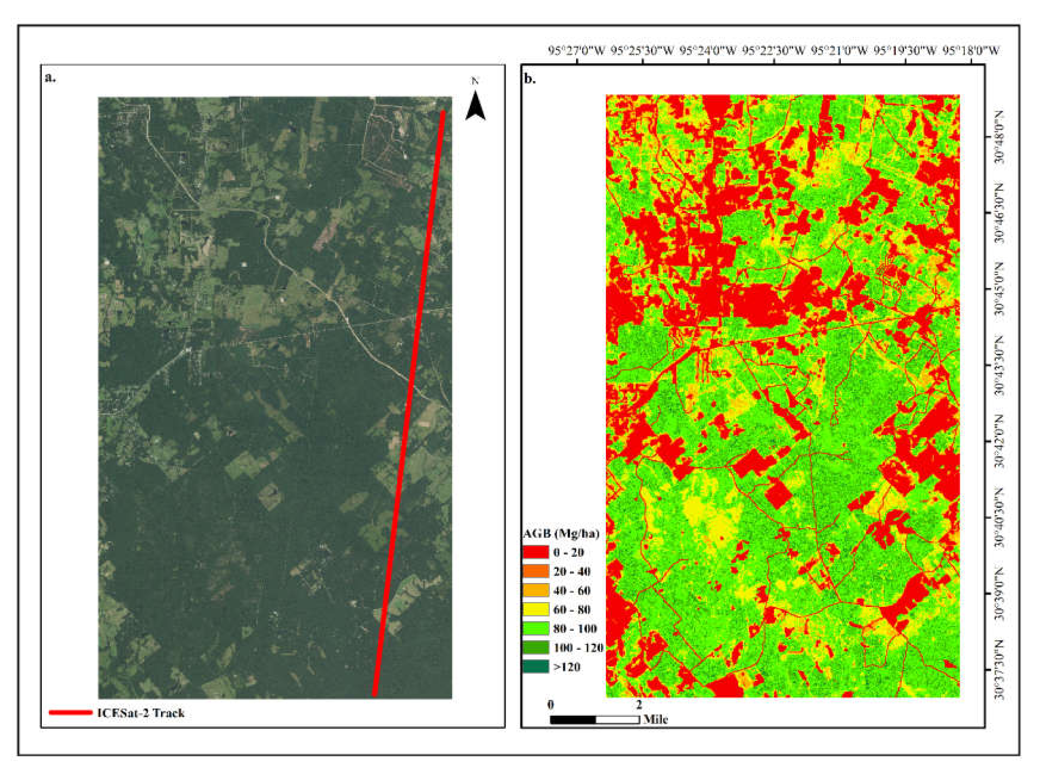
2.5. Mapping AGB with ICESat-2 and Landsat 8 Operational Land Imager (OLI)

While ICESat-2 does not provide comprehensive coverage, the availability of other ancillary and remote-sensing data such as Landsat could be leveraged to achieve mapped products of forest biophysical parameters. Landsat satellites have been providing unprecedented spatial coverage since 1972 and the data, provided at no cost, continues to facilitate scientific research and knowledge advancement [33]. In this study, predicted AGB estimates from 100 m segments along the ICESat-2 transect (strong beam) within the study site were extrapolated to achieve wall-to-wall coverage using spectral indices from a near-cloud-free Landsat 8 OLI imagery (cloud cover less than 0.5%) acquired in April 2019, and NLCD canopy cover and land cover (Table 2). AGB values (strong beam) were assigned to 30 m pixels based on the proportion of the 100-m segment across a pixel. Estimated AGB was then upscaled to represent the 30-m pixel, given the estimated area of the segment within a pixel [16,17]. The machine-learning technique, RF, was used for modeling AGB using the ModelMap R package [25] and the model was evaluated with a separate test set (20% of the data) through R2 and RMSE. The RF model was then applied to upscale ICESat-2 estimated AGB from 720 30-m pixels to produce an AGB map.

3. Results

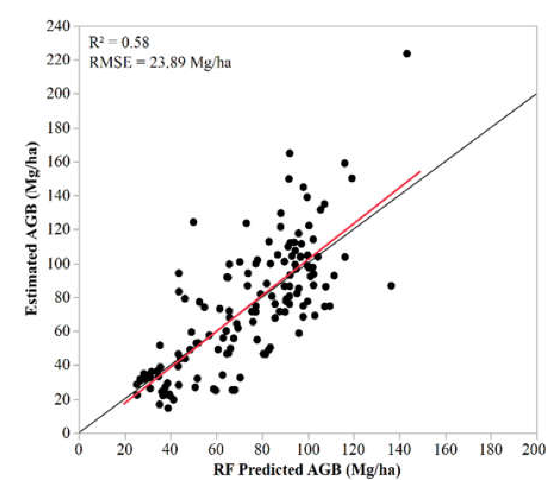
3.1. AGB Estimation Models with ICESat-2

The model for predicting AGB used three height metrics from processed ICESat-2 data (strong beam); mean height, maximum height and the 5th height percentile, with VIFs less than 3. The three-predictor model explained 61% of the variance in the reference AGB used in this study (modeling described in Section 2.2) and yielded a RMSE of 22.15 Mg/ha (Table 2, Figure 4a,b), representing 36% of the dependent mean (reference AGB) of 61.81 Mg/ha. The R2 and RMSE were 0.60 and 24.91 Mg/ha with test data. Notably, an evaluation of correlations between each predictor variable and the dependent variable highlighted strong linear relationships between mean canopy height and AGB (r = 0.77; p-value < 0.0001), as well as between maximum height and AGB (r = 0.59; p-value < 0.0001). The final regression model using AGB estimated with processed ICESat-2 data from the weak beam did not perform as well (Figure 4c,d). The best model used only mean canopy height (p-value < 0.0001) and achieved a R2 and RMSE of 0.41 and 33.73 Mg/ha, respectively, and 0.37 and 35.85 Mg/ha with the test set (Table 3).

3.2. ICESat-2 to Landsat Model

RF model evaluation of predicted AGB (Figure 5), using biomass estimated from ICESat-2-derived metrics (strong beam) as the dependent variable and mapped predictors (Table 2) yielded a R2 and RMSE of 0.58 and 23.89 Mg/ha, with an independent test dataset (144 30-m pixels). Similar to findings with the simulated ICESat-2 vegetation product [17], the most important predictor was canopy cover, with NDVI ranked as the second most important, and least important variable in the model was Modified Soil Adjusted Vegetation Index (MSAVI). Overall, the spatial distribution of predicted AGB density (Figure 6) reflect overall vegetation trends within the study site, with lower values surrounding non-forested areas and predominantly higher biomass in the southern portions which primarily include mature pines. The average RF predicted AGB for the study site was 74.93 Mg/ha and maximum predicted AGB density, 148.96 Mg/ha. The maximum and average AGB values in the training set were 215 Mg/ha and 69.61 Mg/ha respectively. Limitations with using optical remotely sensed data, particularly saturation [34] with increasing AGB, is evident (Figure 5). The integration of other ancillary and radar imagery could be investigated in further research, for improving predictive performance.

4. Discussion

The capability of airborne lidar data to accurately estimate forest structure is well-known [35,36] and with the availability of current spaceborne lidars, crucial information for large-scale mapping and key data for ecological applications can be obtained. Space lidars like ICESat-2 do not replace existing ground inventories but could play an important role in estimating forest structural attributes and enhancing monitoring capability over areas with limited access. Findings from this study serve to provide an initial assessment of ICESat-2 for estimating AGB using available data over forests in south-east Texas. Custom algorithms [11] were applied to geolocated photons in its ATL03 product to retrieve canopy heights and methods were implemented to report canopy metrics in fixed 100 m along-track segments using location information from corresponding ATL08 data, where available. Adapting the methodology previously developed with a simulated ICESat-2 vegetation product [14], results highlight favorable possibilities for using the ICESat-2 measurements to characterize AGB. AGB was predicted well using processed data from the strong beam (R2 = 0.60, RMSE = 24.91 Mg/ha) and while model performance was lower with data from the weak beam (R2 = 0.37, 35.85 Mg/ha), findings suggest that meaningful information can still be obtained. Models developed with the simulated ICESat-2 canopy product for SHNF (strong beam cases only) consisting of similar vegetation conditions, achieved R2 and RMSEs ranging between 0.75 and 0.79 and 19 to 25 Mg/ha, respectively [14].
This study found that relatively few height metrics, mean height and maximum height, contributed substantial information to AGB modeling. Contributions of similar lidar height metrics to AGB estimation models from sensors on airborne platforms are demonstrated in the literature. For instance, Lefsky et al. [37] highlighted mean canopy height extracted from airborne lidar data as the best predictor of AGB in temperate (temperate deciduous and temperate coniferous) and boreal coniferous biomes in the US. In a study by Luo et al. [38], both mean and maximum height parameters from airborne lidar were found to strongly correlate with field-estimated AGB. Essentially, well-established methods developed with airborne lidar data could be used with ICESat-2 data for AGB modeling, after the processing of PCL point clouds demonstrated in this study.
Due to its predictive performance, the model using mean height, maximum height and 5th height percentile from the strong beam was chosen for obtaining ICESat-2-derived AGB estimates, to serve as the dependent variable in the RF model. RF model performance in predicting AGB with vegetation indices from Landsat and NLCD products performed better than expected (R2 = 0.58), given findings with simulated data over SHNF [17]. Spatially explicit estimates exhibit evident spatial patterns in the area; lower biomass in areas surrounding non-forested pixels (e.g., urban areas and roads) and the northern parts of the site and higher values in the southern region, where mature pines are predominant. However, saturation with higher biomass values were noted. Consistent with the biomass mapping studies using optical imagery [38,39], saturation of the signal was evident as AGB levels increased, contributing to underestimated predictions. A combination of data from different sensors and platforms may be necessary to overcome disadvantages associated with each source [40]. The integration of other datasets, including other space-based lidar data from NASA’s Global Ecosystem Dynamics Investigation (GEDI) and ancillary variables such as elevation and climatic information, is recommended for further upscaling efforts.
The availability of space-based lidar data from two missions, ICESat-2 and GEDI, launched around the same time (in 2018), is extraordinary. As more ICESat-2 tracks and data from NASA’s GEDI lidar 2-year mission become available, there will be opportunities for integrating data from multiple spaceborne missions to potentially derive more accurate products. GEDI was designed to capture structural information of forest ecosystems between 52°N and S latitudes and therefore represents a critical source of measurements [41]. Duncanson et al. [42] recently compared biomass estimates from GEDI and ICESat-2 with a reference airborne lidar AGB map, using simulated data for both missions over Sanoma County, California. The RMSE values ranged from 80.2 Mg/ha to 128.8 Mg/ha (% RMSE= 64.5% to 87.6%) with simulated GEDI data and with ICESat-2, 106.4 Mg/ha and 137.8 Mg/ha (% RMSE = 59% and 89.1%) for high and low photon return scenarios, respectively. With ICESat-2 providing near-global coverage and GEDI focused on mid-latitude regions, approaches for incorporating both datasets with other sources, would be essential for achieving global coverage products. In doing so, algorithms optimized for handling large datasets, such as deep-learning approaches, could be investigated.
Limitations in our study, contributing to errors in modeling AGB, are noted. First, with the lack of ground reference data spatially coincident with the ICESat-2 transect, an available airborne lidar-derived AGB map (using ground and airborne lidar data) for SHNF was upscaled to serve as a reference. It is important to mention, though, that the upscaled map strongly correlated with the existing airborne lidar-derived AGB estimates for SHNF. Second, temporal inconsistencies exist between reference AGB and ICESat-2 data; the available AGB map for SHNF was developed with airborne lidar data collected in 2010. A significant factor here is that upscaling to encompass the ICESat-2 transect was done using spectral indices from imagery collected around the same time, from 2010-2011 and NLCD products from 2011. Wall-to-wall mapping with ICESat-2-derived AGB was later carried out with vegetation indices calculated using Landsat 8 OLI imagery, approximately temporally coincident with the ICESat-2 measurements. A comprehensive uncertainty analysis, to account for errors arising from each modeling step (e.g., Saarela et al. [43]), is recommended, especially for mapping over larger extents.
ICESat-2 will provide near-global coverage and with other available Earth observations, such as Landsat, global-scale characterization of forest structural parameters, including updated canopy heights and AGB maps, can be investigated. This initial work serves to highlight the application of ICESat-2 data for biomass studies. Further research will seek to refine and develop approaches to integrate ICESat-2’s PCL data for characterizing forest structure over larger spatial extents.

5. Conclusions

This study provides an initial assessment of ICESat-2 for estimating forest aboveground biomass (AGB) over forests in southeast Texas, and findings that support a methodology for estimating biomass with the mission’s PCL data. Using ICESat-2’s geolocated photon data, custom algorithms were applied to derive canopy heights from both strong and weak beams over the study site. The data were further processed to report a range of canopy height metrics in 100 m × 17 m segments in the along-track direction. Canopy parameters from segments were used to estimate AGB, yielding a R2 of 0.41 and 0.61 with the weak and strong beams, respectively. Extrapolation of ICESat-2-derived AGB estimates from segments along the ICESat-2 transect, to 30 m pixels across the study site was carried out with RF, using Landsat and NLCD products. Results are indicative of the utility of ICESat-2 data for characterizing AGB. As more ICESat-2 tracks become available and with the availability of corresponding reference data, an improved understanding of the data and their ability to characterize vegetation structure will be gleaned. Nonetheless, possibilities with the data, including synergistic use with freely available data from other space-based missions, including GEDI, are exciting. Future work will involve the application of the methodology for regional-scale mapping with corresponding uncertainty analyses and an investigation of deep-learning approaches with multi-source data.

Author Contributions

Conceptualization, S.C.P., L.L.N.; methodology, L.L.N. and S.C.P.; formal analysis, L.L.N.; investigation, L.L.N. and L.M.; resources, S.C.P. and L.L.N.; writing—original draft preparation, L.L.N.; writing—review and editing, L.L.N., S.C.P. and L.M.; visualization, L.L.N. and L.M. All authors have read and agreed to the published version of the manuscript.

Funding

This research was supported by the School of Forestry and Wildlife Sciences at Auburn University and NASA Science Team grant NNH192DA001N.

Acknowledgments

We sincerely thank Shruthi Srinivasan with the Texas Forest Service for her contributions to the reference biomass map for the Sam Houston National Forest. We are also grateful for the constructive and comprehensive reviews provided by reviewers.

Conflicts of Interest

The authors declare no conflict of interest.

References

  1. Hall, F.G.; Bergen, K.; Blair, J.B.; Dubayah, R.; Houghton, R.; Hurtt, G.; Kellndorfer, J.; Lefsky, M.; Ranson, J.; Saatchi, S.; et al. Characterizing 3D vegetation structure from space: Mission requirements. Remote Sens. Environ. 2011, 115, 2753–2775. [Google Scholar] [CrossRef] [Green Version]
  2. Markus, T.; Neumann, T.; Martino, A.; Abdalati, W.; Brunt, K.; Csatho, B.; Farrell, S.; Fricker, H.; Gardner, A.; Harding, D.; et al. The Ice, Cloud, and land Elevation Satellite-2 (ICESat-2): Science requirements, concept, and implementation. Remote Sens. Environ. 2017, 190, 260–273. [Google Scholar] [CrossRef]
  3. Lefsky, M.A. A global forest canopy height map from the Moderate Resolution Imaging Spectroradiometer and the Geoscience Laser Altimeter System. Geophys. Res. Lett. 2010, 37, 5. [Google Scholar] [CrossRef] [Green Version]
  4. Simard, M.; Pinto, N.; Fisher, J.B.; Baccini, A. Mapping forest canopy height globally with spaceborne lidar. J. Geophys. Res. Biogeosciences 2011, 116, 12. [Google Scholar] [CrossRef]
  5. Chi, H.; Sun, G.Q.; Huang, J.L.; Guo, Z.F.; Ni, W.J.; Fu, A.M. National Forest Aboveground Biomass Mapping from ICESat/GLAS Data and MODIS Imagery in China. Remote Sens. 2015, 7, 5534–5564. [Google Scholar] [CrossRef] [Green Version]
  6. Hu, T.; Su, Y.; Xue, B.; Liu, J.; Zhao, X.; Fang, J.; Guo, Q. Mapping Global Forest Aboveground Biomass with Spaceborne LiDAR, Optical Imagery, and Forest Inventory Data. Remote Sens. 2016, 8, 565. [Google Scholar] [CrossRef] [Green Version]
  7. Yang, X.B.; Wang, C.; Pan, F.F.; Nie, S.; Xi, X.H.; Luo, S.Z. Retrieving leaf area index in discontinuous forest using ICESat/GLAS full-waveform data based on gap fraction model. ISPRS J. Photogramm. Remote Sens. 2019, 148, 54–62. [Google Scholar] [CrossRef]
  8. Pourrahmati, M.R.; Baghdadi, N.N.; Darvishsefat, A.A.; Namiranian, M.; Fayad, I.; Bailly, J.; Gond, V. Capability of GLAS/ICESat Data to Estimate Forest Canopy Height and Volume in Mountainous Forests of Iran. IEEE J. Sel. Top. Appl. Earth Obs. Remote Sens. 2015, 8, 5246–5261. [Google Scholar] [CrossRef] [Green Version]
  9. Neuenschwander, A.L.; Magruder, L.A. The Potential Impact of Vertical Sampling Uncertainty on ICESat-2/ATLAS Terrain and Canopy Height Retrievals for Multiple Ecosystems. Remote Sens. 2016, 8, 1039. [Google Scholar] [CrossRef] [Green Version]
  10. Neuenschwander, A.; Pitts, K. The ATL08 land and vegetation product for the ICESat-2 Mission. Remote Sens. Environ. 2019, 221, 247–259. [Google Scholar] [CrossRef]
  11. Popescu, S.C.; Zhou, T.; Nelson, R.; Neuenschwander, A.; Sheridan, R.; Narine, L.; Walsh, K.M. Photon counting LiDAR: An adaptive ground and canopy height retrieval algorithm for ICESat-2 data. Remote Sens. Environ. 2018, 208, 154–170. [Google Scholar] [CrossRef]
  12. Gwenzi, D.; Lefsky, M.A.; Suchdeo, V.P.; Harding, D.J. Prospects of the ICESat-2 laser altimetry mission for savanna ecosystem structural studies based on airborne simulation data. ISPRS J. Photogramm. Remote Sens. 2016, 118, 68–82. [Google Scholar] [CrossRef]
  13. Glenn, N.F.; Neuenschwander, A.; Vierling, L.A.; Spaete, L.; Li, A.H.; Shinneman, D.J.; Pilliod, D.S.; Arkle, R.S.; McIlroy, S.K. Landsat 8 and ICESat-2: Performance and potential synergies for quantifying dryland ecosystem vegetation cover and biomass. Remote Sens. Environ. 2016, 185, 233–242. [Google Scholar] [CrossRef]
  14. Narine, L.L.; Popescu, S.; Neuenschwander, A.; Zhou, T.; Srinivasan, S.; Harbeck, K. Estimating aboveground biomass and forest canopy cover with simulated ICESat-2 data. Remote Sens. Environ. 2019, 224, 1–11. [Google Scholar] [CrossRef]
  15. Neuenschwander, A.L.; Magruder, L.A. Canopy and Terrain Height Retrievals with ICESat-2: A First Look. Remote Sens. 2019, 11, 1721. [Google Scholar] [CrossRef] [Green Version]
  16. Narine, L.L.; Popescu, S.C.; Malambo, L. Synergy of ICESat-2 and Landsat for Mapping Forest Aboveground Biomass with Deep Learning. Remote Sens. 2019, 11, 1503. [Google Scholar] [CrossRef]
  17. Narine, L.L.; Popescu, S.; Zhou, T.; Srinivasan, S.; Harbeck, K. Mapping forest aboveground biomass with a simulated ICESat-2 vegetation canopy product and Landsat data. Ann. For. Res. 2019, 62. [Google Scholar] [CrossRef]
  18. Yang, L.; Jin, S.; Danielson, P.; Homer, C.; Gass, L.; Bender, S.M.; Case, A.; Costello, C.; Dewitz, J.; Fry, J.; et al. A new generation of the United States National Land Cover Database: Requirements, research priorities, design, and implementation strategies. ISPRS J. Photogramm. Remote Sens. 2018, 146, 108–123. [Google Scholar] [CrossRef]
  19. MRLC. Multi-Resolution Land Characteristics (MRLC) Consortium. Available online: https://www.mrlc.gov/ (accessed on 3 June 2020).
  20. Popescu, S.C.; Wynne, R.H.; Nelson, R.F. Measuring individual tree crown diameter with lidar and assessing its influence on estimating forest volume and biomass. Can. J. Remote Sens. 2003, 29, 564–577. [Google Scholar] [CrossRef]
  21. Popescu, S.C.; Wynne, R.H. Seeing the trees in the forest: Using lidar and multispectral data fusion with local filtering and variable window size for estimating tree height. Photogramm. Eng. Remote Sens. 2004, 70, 589–604. [Google Scholar] [CrossRef] [Green Version]
  22. Jenkins, J.C.; Chojnacky, D.C.; Heath, L.S.; Birdsey, R.A. National-scale biomass estimators for United States tree species. For. Sci. 2003, 49, 12–35. [Google Scholar]
  23. Snyder, K.A.; Huntington, J.L.; Wehan, B.L.; Morton, C.G.; Stringham, T.K. Comparison of Landsat and Land-Based Phenology Camera Normalized Difference Vegetation Index (NDVI) for Dominant Plant Communities in the Great Basin. Sensors 2019, 19, 1139. [Google Scholar] [CrossRef] [PubMed] [Green Version]
  24. Ikasari, I.H.; Ayumi, V.; Fanany, M.I.; Mulyono, S. Multiple Regularizations Deep Learning for Paddy Growth Stages Classification from LANDSAT-8. In Proceedings of the 2016 International Conference on Advanced Computer Science and Information Systems, Malang, Indonesia, 15–16 October 2016; IEEE: New York, NY, USA, 2016; pp. 512–517. [Google Scholar]
  25. Freeman, E.A.; Frescino, T.S.; Moisen, G.G. ModelMap: An R Package for Model Creation and Map Production; USDA Forest Service, Rocky Montains Research Station: Ogden, UT, USA, 2018; p. 69. [Google Scholar]
  26. Neumann, T.A.; Brenner, A.; Hancock, D.; Robbins, J.; Luthcke, S.B.; Harbeck, K.; Lee, J.; Gibbons, A.; Saba, J.; Brunt, K.M. ATLAS/ICESat-2 L2A Global Geolocated Photon Data, Version 1; NSIDC: National Snow and Ice Data Center: Boulder, CO, USA, 2019. [Google Scholar] [CrossRef]
  27. Neuenschwander, A.L.; Popescu, S.C.; Nelson, R.F.; Harding, D.; Pitts, K.L.; Robbins, J. ATLAS/ICESat-2 L3A Land and Vegetation Height, Version 1; NSIDC: National Snow and Ice Data Center: Boulder, CO, USA, 2019. [Google Scholar] [CrossRef]
  28. Neumann, T.A.; Martino, A.J.; Markus, T.; Bae, S.; Bock, M.R.; Brenner, A.C.; Brunt, K.M.; Cavanaugh, J.; Fernandes, S.T.; Hancock, D.W.; et al. The Ice, Cloud, and Land Elevation Satellite—2 mission: A global geolocated photon product derived from the Advanced Topographic Laser Altimeter System. Remote Sens. Environ. 2019, 233, 111325. [Google Scholar] [CrossRef] [PubMed]
  29. Moussavi, M.S.; Abdalati, W.; Scambos, T.; Neuenschwander, A. Applicability of an automatic surface detection approach to micropulse photon-counting lidar altimetry data: Implications for canopy height retrieval from future ICESat-2 data. Int. J. Remote Sens. 2014, 35, 5263–5279. [Google Scholar] [CrossRef]
  30. Isenburg, M. LASTools: Award-Winning Software for Rapid LiDAR Processing. Available online: http://lastools.org/ (accessed on 25 February 2020).
  31. McGaughey, R.J. FUSION/LDV: Software for LIDAR Data Analysis and Visualization; US Department of Agriculture, Forest Service, Pacific Northwest Research Station: Seattle, WA, USA, 2016.
  32. Nelson, R.; Margolis, H.; Montesano, P.; Sun, G.; Cook, B.; Corp, L.; Andersen, H.-E.; de Jong, B.; Pellat, F.P.; Fickel, T.; et al. Lidar-based estimates of aboveground biomass in the continental US and Mexico using ground, airborne, and satellite observations. Remote Sens. Environ. 2017, 188, 127–140. [Google Scholar] [CrossRef] [Green Version]
  33. Wulder, M.A.; Loveland, T.R.; Roy, D.P.; Crawford, C.J.; Masek, J.G.; Woodcock, C.E.; Allen, R.G.; Anderson, M.C.; Belward, A.S.; Cohen, W.B.; et al. Current status of Landsat program, science, and applications. Remote Sens. Environ. 2019, 225, 127–147. [Google Scholar] [CrossRef]
  34. Zhu, X.; Liu, D. Improving forest aboveground biomass estimation using seasonal Landsat NDVI time-series. ISPRS J. Photogramm. Remote Sens. 2015, 102, 222–231. [Google Scholar] [CrossRef]
  35. Bae, S.; Levick, S.R.; Heidrich, L.; Magdon, P.; Leutner, B.F.; Wöllauer, S.; Serebryanyk, A.; Nauss, T.; Krzystek, P.; Gossner, M.M.; et al. Radar vision in the mapping of forest biodiversity from space. Nat. Commun. 2019, 10, 4757. [Google Scholar] [CrossRef]
  36. Popescu, S.C. Estimating biomass of individual pine trees using airborne lidar. Biomass Bioenergy 2007, 31, 646–655. [Google Scholar] [CrossRef]
  37. Lefsky, M.A.; Cohen, W.B.; Harding, D.J.; Parker, G.G.; Acker, S.A.; Gower, S.T. Lidar remote sensing of above-ground biomass in three biomes. Glob. Ecol. Biogeogr. 2002, 11, 393–399. [Google Scholar] [CrossRef] [Green Version]
  38. Luo, S.; Wang, C.; Xi, X.; Pan, F.; Peng, D.; Zou, J.; Nie, S.; Qin, H. Fusion of airborne LiDAR data and hyperspectral imagery for aboveground and belowground forest biomass estimation. Ecol. Indic. 2017, 73, 378–387. [Google Scholar] [CrossRef]
  39. Avitabile, V.; Baccini, A.; Friedl, M.A.; Schmullius, C. Capabilities and limitations of Landsat and land cover data for aboveground woody biomass estimation of Uganda. Remote Sens. Environ. 2012, 117, 366–380. [Google Scholar] [CrossRef]
  40. Rodríguez-Veiga, P.; Wheeler, J.; Louis, V.; Tansey, K.; Balzter, H. Quantifying Forest Biomass Carbon Stocks From Space. Curr. For. Rep. 2017, 3, 1–18. [Google Scholar] [CrossRef] [Green Version]
  41. Dubayah, R.; Blair, J.B.; Goetz, S.; Fatoyinbo, L.; Hansen, M.; Healey, S.; Hofton, M.; Hurtt, G.; Kellner, J.; Luthcke, S.; et al. The Global Ecosystem Dynamics Investigation: High-resolution laser ranging of the Earth’s forests and topography. Sci. Remote Sens. 2020, 1, 100002. [Google Scholar] [CrossRef]
  42. Duncanson, L.; Neuenschwander, A.; Hancock, S.; Thomas, N.; Fatoyinbo, T.; Simard, M.; Silva, C.A.; Armston, J.; Luthcke, S.B.; Hofton, M.; et al. Biomass estimation from simulated GEDI, ICESat-2 and NISAR across environmental gradients in Sonoma County, California. Remote Sens. Environ. 2020, 242, 111779. [Google Scholar] [CrossRef]
  43. Saarela, S.; Holm, S.; Healey, S.P.; Andersen, H.-E.; Petersson, H.; Prentius, W.; Patterson, P.L.; Næsset, E.; Gregoire, T.G.; Ståhl, G. Generalized Hierarchical Model-Based Estimation for Aboveground Biomass Assessment Using GEDI and Landsat Data. Remote Sens. 2018, 10, 1832. [Google Scholar] [CrossRef] [Green Version]
Figure 1. An overview of methods used in this study.
Remotesensing 12 01824 g001
Figure 2. (a) Map of Texas with the study site highlighted; (b) a 13-mile Ice, Cloud, and land Elevation Satellite-2 (ICESat-2) transect (GT3R) overlaid on a reference aboveground biomass map (biomass density in Mg/ha) for the study area and showing simulated ICESat-2 tracks (yellow) over the extent of Sam Houston National Forest (SHNF) within the study site. The map uses a gray-scale symbology, where lighter pixels represent higher levels of biomass. Non-forested areas have been masked.
Remotesensing 12 01824 g002
Figure 3. (a) Profile of raw ICESat-2 (ATL03) data from the strong beam of track 3 (GT3R) over temperate forests in southeast Texas; (b) profile of filtered and classified data from GT3R; (c) raw and processed ICESat-2 data for a subset of the profile from the strong beam of track 3 (GT3R); (d) profile of raw ICESat-2 (ATL03) data from the weak beam of track 3 (GT3L) over temperate forests in southeast Texas; (e) profile of filtered and classified data from GT3L; (f) raw and processed ICESat-2 data for a subset of the profile from the weak beam of track 3 (GT3L) These data were acquired on 3 December 2018; granule ID ATL03_20181203072948_10030106_002_01.
Remotesensing 12 01824 g003aRemotesensing 12 01824 g003b
Figure 4. (a) Reference AGB versus ICESat-2-predicted AGB (Mg/ha) with training data, for the strong beam; (b) reference AGB versus ICESat-2-predicted AGB (Mg/ha) with test data, for the strong beam; (c) reference AGB versus ICESat-2-predicted AGB (Mg/ha) with training data, for the weak beam; (d) reference AGB versus ICESat-2-predicted AGB (Mg/ha) with test data, for the weak beam. The solid black line in each graph is the 1:1 line.
Remotesensing 12 01824 g004
Figure 5. Scatterplot showing the relationship between ICESat-2 derived AGB and random forest (RF) predicted AGB with test data.
Remotesensing 12 01824 g005
Figure 6. (a) Map of study area showing ICESat-2 transect analyzed, overlaid on 2016 natural color National Agriculture Imagery Program (NAIP) imagery; (b) predicted AGB density for the study area (30 m grid size).
Remotesensing 12 01824 g006
Table 1. ICESat-2-derived metrics used for estimating AGB.
Independent VariableDescription
MinMinimum height
MaxMaximum height
MeanMean height
P1010th percentile height
P2525th percentile height
P5050th percentile height
P7070th percentile height
P7575th percentile height
P8080th percentile height
P9090th percentile height
P9595th percentile height
P9999th percentile height
C2mPercentage of all returns above 2m
Table 2. Metrics derived from Landsat 8 Operational Land Imager (OLI) and National Land Cover Database (NLCD) landcover and canopy cover, for upscaling ICESat-2-derived AGB.
Independent VariableDescription
Normalized Difference Vegetation Index (NDVI)(near infrared (NIR) - Red) / (NIR + Red)
Enhanced Vegetation Index (EVI) 2.5 * ((NIR - Red) / (NIR + 6 * Red - 7.5 * Blue + 1))
Soil Adjusted Vegetation Index (SAVI) ((NIR - Red) / (NIR + Red + 0.5)) * (1.5)
Modified Soil Adjusted Vegetation Index (MSAVI)(2 * NIR + 1 - sqrt ((2 * NIR + 1)2 - 8 * (NIR - Red))) / 2
Land coverLand cover map from the National Land Cover Databased (NLCD) 2016
Canopy coverNLCD 2011 US Forest Service Tree Canopy Cover
Table 3. Regression models for estimating AGB with ICESat-2 data from the strong beam and weak beam.
ICESat-2 BeamDependent VariablePredictorsRoom Mean Square Error (RMSE)R2Model
TrainingTestTrainingTest
Strong beam (GT3R)AGB (Mg/ha)Maximum height, mean height, 5th percentile height22.15 Mg/ha24.91 Mg/ha0.610.6020.56 – 0.26Max + 5.95Mean – 7.14p05
Weak beam (GT3L)AGB (Mg/ha)Mean height33.73 Mg/ha35.85 Mg/ha0.410.3711.72 + 4.31Mean

