Article

Assessing the Effects of Photovoltaic Powerplants on Surface Temperature Using Remote Sensing Techniques

1
Key Laboratory of Geospatial Technology for the Middle and Lower Yellow River Regions, Henan University, Ministry of Education, Kaifeng 475004, China
2
College of Environment and Planning, Henan University, Kaifeng 475004, China
*
Author to whom correspondence should be addressed.
Remote Sens. 2020, 12(11), 1825; https://doi.org/10.3390/rs12111825
Submission received: 18 April 2020 / Revised: 22 May 2020 / Accepted: 28 May 2020 / Published: 5 June 2020
(This article belongs to the Special Issue Remote Sensing for Biometeorology)

Abstract

:
The rapid development of photovoltaic (PV) powerplants in the world has drawn attention on their climate and environmental impacts. In this study, we assessed the effects of PV powerplants on surface temperature using 23 largest PV powerplants in the world with thermal infrared remote sensing technique. Our result showed that the installation of the PV powerplants had significantly reduced the daily mean surface temperature by 0.53 °C in the PV powerplant areas. The cooling effect with the installation of the PV powerplants was much stronger during the daytime than the nighttime with the surface temperature dropped by 0.81 °C and 0.24 °C respectively. This cooling effect was also depended on the capacity of the powerplants with a cooling rate of −0.32, −0.48, and −0.14 °C/TWh, respectively, for daily mean, daytime, and nighttime temperature. We also found that the construction of the powerplants significantly decreased the surface albedo from 0.22 to 0.184, but significantly increased the effective albedo (surface albedo plus electricity conversion) from 0.22 to 0.244, suggesting conversion of solar energy to electrical energy is a major contributor to the observed surface cooling. Our further analyses showed that the nighttime cooling in the powerplants was significantly correlated with the latitude and elevation of the powerplants as well as the annual mean temperature, precipitation, solar radiation, and normalized difference vegetation index (NDVI). This means the temperature effect of the PV powerplants depended on regional geography, climate and vegetation conditions. This finding can be used to guide the selection of the sites of PV powerplants in the future.

Graphical Abstract

1. Introduction

Solar power is the most abundantly available renewable energy source which has a great potential to substitute fossil-fuel and thus reduces green-house gas (GHG) emissions [1,2]. With the advances in photovoltaic (PV) technique, solar energy can be directly converted into electrical energy and solar powerplants have become as economically efficient as traditional fossil-fuel powerplants [3,4,5]. According to the International Energy Agency (IEA), the global installed PV capacity has increased from about 100,000 KW in 1992 to more than 500 million KW in 2018. The large-scale installation of solar PV panels has a direct impact on local and possibly regional climate in addition to its indirect climate effect by reducing GHG [6,7]. The GHG reduction effects on solar powerplants has been well studied through life-cycle assessment (LCA) in the past decades [2,8,9,10,11,12,13,14]. But few studies have focused on investigating the direct impact of the PV powerplants on climate, which is important for fully assessing the impacts of solar powerplants on climate and environment.
Temperature, as manifestation of thermal energy, is the most important factor to reflect the variation of energy balance. Due to interactions among energy budget, water cycle and vegetation growth on the PV powerplant is still unclear over different regions, the PV temperature effect has become a controversial issue. Some studies have found that rooftop PV panels can reduce daytime air temperature by 0.2–0.8 °C during the summer in urban areas [6,15,16]. However, there is no consistent conclusion for the large-scale PV powerplants which may have cooling [17] or warming effects [18,19] according to earlier studies. Nevertheless, recent field observations showed that the PV powerplants in arid regions could increase daytime air temperature up to 9.7 °C [20,21,22,23]. Meanwhile, some model-based simulations have shown that PV powerplants could reduce daytime air temperature considerably [6,17]. In drylands of northwest China and northwest America, the effect of PV powerplants on nighttime temperature is also uncertain with warming [21,22], cooling [23] or non-significant effects [20] reported in literature. The air temperature at the PV powerplants is often measured with a standard weather station where temperature sensors are installed at a height of 1.5 m or 2 m above the ground [20,21,23]. Thus the air temperature measured at different PV powerplants may be affected by the solar panels installed at different heights. The air temperature measured at PV powerplants may also be biased due to the small “footprints” of the weather stations and the high heterogeneity of surface conditions.
The land or skin surface temperature is one of the key climate variables determined by the surface energy balance and closely related to the near surface air temperature [24,25,26,27,28,29]. Unlike air temperature measured by weather stations as point samples, surface temperature can be monitored using satellite remote sensing with a much larger spatial coverage [30]. Previous studies have found that remote sensing platforms, such as AVHRR, MODIS and Landsat, can be used to map land surface temperature effectively in various regions [26,31,32,33,34,35,36,37,38,39]. But this technique has not been attempted to map the surface temperature in PV powerplants (the surface temperature is the mixture of PV panels surface temperature and the surface temperature of land between solar panels).
In this study, we used the EOS-MODIS thermal band [40], which had high temporal and spatial resolution and long term remote sensing observations, to investigate the effects of the PV powerplants on surface temperature using 23 largest PV powerplants in the world. We processed the remote sensing images in Google Earth Engine, which is a cloud-based platform with massive computational capabilities for processing spatial-temporal data [41].
Specifically, the main objectives of this study are to: (1) assess the effects of the installation of the PV powerplants on daytime, nighttime and daily surface temperature; and (2) further examine if these effects are related to location, local climate and surface conditions.

2. Materials and Methods

2.1. Study Area and the Photovoltaic (PV) Powerplants Selection

We use the MODIS thermal band to map the surface temperature and thus the minimum size of PV powerplants should cover at least 9 pixels of the MODIS thermal band which has a spatial resolution of 1000 meters. In addition to the size of the PV powerplants, site conditions, such as homogeneity of land cover and topography, are also important in selecting the candidates of PV powerplants. Therefore, we used Landsat 8 data (Tier 1, Collection 1) with a resolution of 30 m to identify and delineate the PV powerplants in 2018. We mapped the extents of each PV powerplant by visual interpretation in ArcGIS 10.5. As a result, we selected 23 among the largest PV powerplants in the world with minimum variation in land cover and topography in their adjacent surroundings (Table 1). Based on the geo-referenced data, we extracted the basic information, such as located country, powerplant area, mean altitude above sea level (a.s.l), longitude and latitude, of each PV powerplant (Table 1). The mean altitude of each PV site was derived from the SRTM-DEM dataset with a 30 m spatial resolution (Farr et al., 2007). We also extracted the longterm yearly average potential PV electricity production per unit capacity (KWh/KWp) with 30 arc seconds (about 1 km) resolution from the Global Solar Atlas dataset [42].With the installed capacity density (50,000 KW/Km2), we also calculated the potential annual electricity production of each PV powerplant [43]. As shown in Table 1, the 23 selected PV powerplants are mainly distributed in the northern hemisphere with latitudes ranging from 9.32° to 43.12°, areas varying between 5.4 km2 to 91.9 km2 and altitude ranging from 9.6 to 2985.6 m.a.s.l. Details of the 23 selected PV powerplants are listed in Table 1.

2.2. Quantifying the Effects of the PV Powerplants on Surface Temperature

The MODIS Land surface temperature (LST), level-3, collection-6 provides products with a global coverage of 4 times (local passing the equator at 10:30 and 22:30 local time for Terra and 1:30 and 13:30 local time for Aqua) every day since 2002 [30]. The surface temperature was derived from clear-sky (99% confidence) observations using a generalized split windows algorithm from MODIS channel 31 and channel 32 with a spectral wavelength centering at 11 µm and 12 µm, respectively [44,45]. The noise equivalent temperature difference (NEDT) of MODIS channel 31 and channel 32 is 0.05 K [46]. In the current study, we used the MOD11A2 of Terra and MYD11A2 of Aqua datasets with a 1-km spatial resolution and 8-day average LST [24,47]. We excluded the data with average emissivity error larger than 0.02 and average LST error larger than 2 K (provided by the quality control band) from our analysis. We first calculated the daytime surface temperature by averaging the surface temperatures measured at 10:30 and 13:30 (satellite passing time) and nighttime surface temperature by averaging the temperatures measured at 22:30 and 1:30. We further calculated the average surface temperature of each PV powerplant by averaging the surface temperature of each pixel within the PV powerplant.
We used the temperature difference, the surface temperature after the establishment of the powerplant minus the temperature before the establishment, as an indicator to quantify the powerplant effect on surface temperature. It is noted that most of the powerplants started installation and operation in different years and some of them took more than a year to establish. The surface temperature normally saw an abrupt change with installation of PV powerplants as evidenced in our preliminary study (Figure 1). Therefore, we took advantage of the time series of temperature data and used the Breaks For Additive Season and Trend (BFAST) method in R language [48] to detect abrupt changes in the surface temperature (daily mean, daytime and nighttime) for determining the starting and ending construction time of each PV powerplant (Figure 1).The starting and ending time of each powerplant was also confirmed by the time series of Landsat images and the Google Earth images. We used the mean surface temperature of 2018 as the post-construction period temperature because all the selected powerplants finished their construction before 2018. We used a three-year-averaged (calendar year) temperature before the construction of each powerplant as our prior reference temperature (Figure 1).
Given the fact that temperature changes among years especially under global climate change, we used a 2 km buffer (control area) around each powerplant as a spatial reference to eliminate surface temperature changes in time assuming the control area has not been affected by the installation of the PV powerplant. This assumption is confirmed by the vegetation data and our visualization of the high-resolution Google Earth images. The control areas were created using R language. The change of surface temperature (after vs. before the construction of PV powerplant) in the control area was calculated the same as within the powerplant. Finally, the effect of PV powerplants on surface temperature was calculated as:
PVPPTE = (TpaTpb) − (TcaTcb)
where PVPPTE is PV powerplant temperature effect (°C), Tpa is the powerplant surface temperature after its establishment (°C), Tpb is the powerplant surface temperature before its construction (°C), Tca is the control surface temperature after the establishment of the powerplant (°C), and Tcb is the control surface temperature before the construction of the powerplant (°C). To calculate the PVPPTE could also minimize the difference in radiative transfer length in the atmospheric profiles, the directional emissivity of heterogeneous surface, and the pixel size in different viewing angle and time.

2.3. Normalized Difference Vegetation Index (NDVI) and Albedo Data

We used the normalized difference vegetation index (NDVI) and albedo data to examine if the temperature effect of PV powerplant is related to the pre-construction surface condition. Those data were also used to assess the impacts of the installation of PV powerplants on vegetation and surface energy budgets. The NDVI were derived from the MODIS, level-3, collection-6 MOD13A1 product with a 500 m spatial resolution. As a commonly accepted method, we used the 16-day composite data in this study to remove the impact of clouds [49,50]. The surface albedo data were derived from the MODIS, level-3, collection-6 MCD43A3 product with a 500 m spatial resolution and daily temporal resolution. We used the same approach as in Li, et al. [51] to process the albedo data. Similar to surface temperature, we calculated the PV powerplant effects on NDVI and albedo by using the 3-year average NDVI and albedo before the construction of the PV powerplant and the post-construction NDVI and albedo in 2018.

2.4. Climate Factors

In this study, we also investigated if the local climate conditions, such as yearly air temperature, precipitation, solar radiation, vapor pressure and wind speed, are related to the surface temperature effect of the PV powerplants (Table 2). We downloaded the 30 arc seconds (about 1 km) climate data from the WorldClim (version 2.0) dataset which has been widely tested and used in many studies [52,53,54,55]. We also downloaded the latest ERA reanalysis climate data with a spatial resolution of 0.25 arc degrees (about 25 km) [56] to analyze the changes in climate variables before and after the installation of the PV powerplants.

3. Results

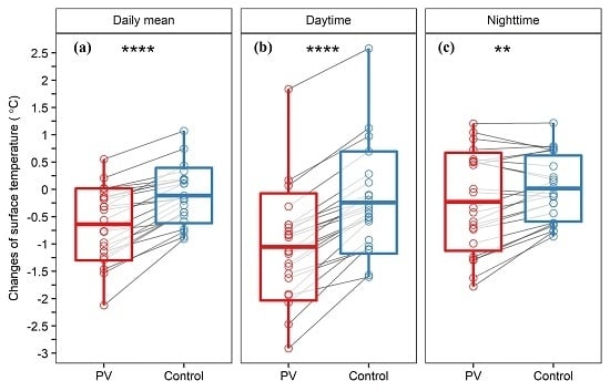
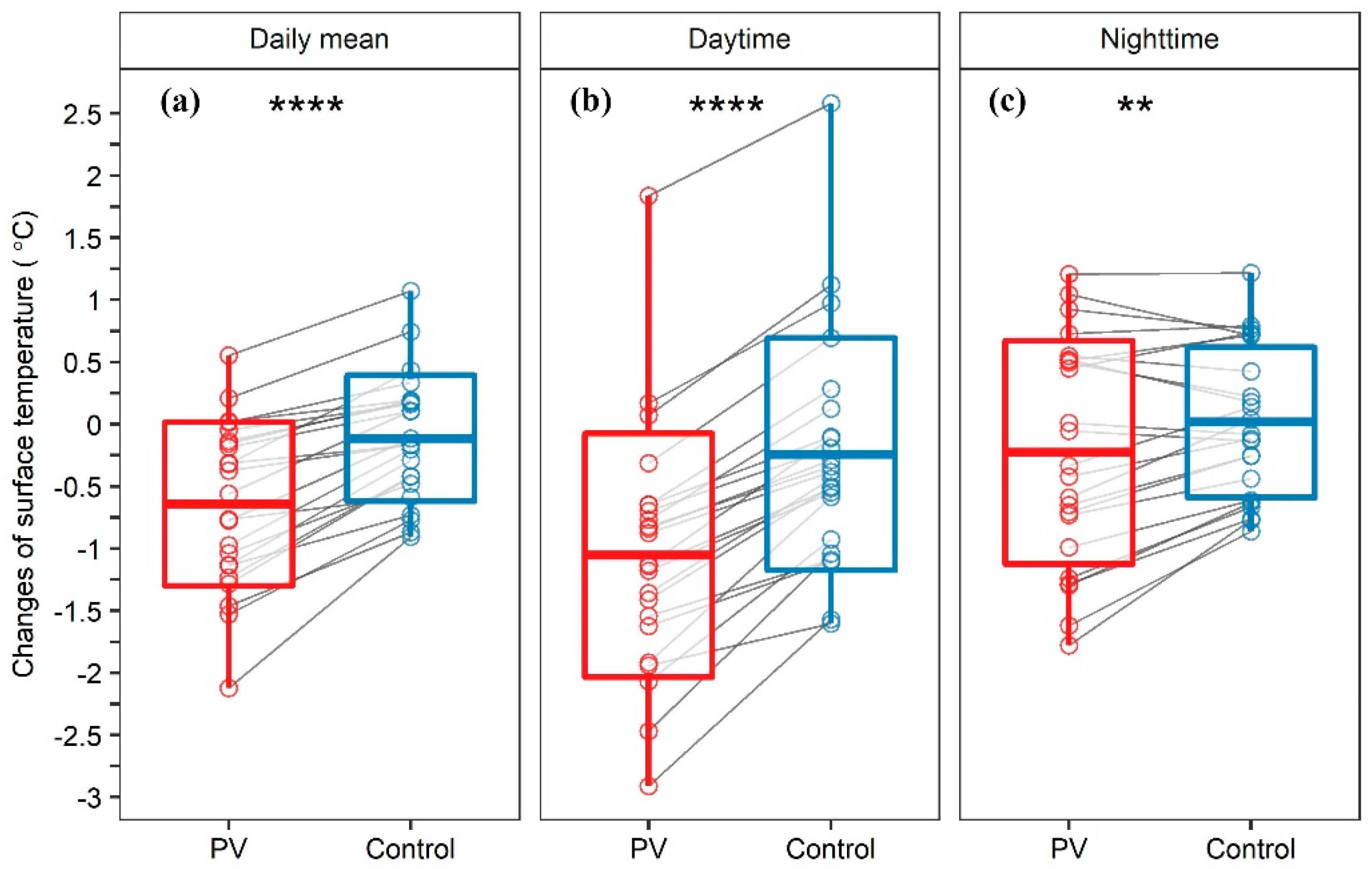
3.1. The Effects of Photovoltaic (PV) Powerplants on Surface Temperature

We found that the installation of the PV powerplants significantly (p < 0.0001) reduced the annual mean surface temperature (average of daytime and nighttime surface temperatures), a cooling effect, by 0.53 °C with the mean surface temperature in the PV powerplants decreasing 0.64 °C, from 21.48 to 20.84 °C, while the surface temperature in the control zones decreased 0.11 °C, from 21.41 to 21.3 °C (Figure 2a) (Table 3). We also found that the mean surface temperature in the control zones was not statistically different before and after the establishment of the PV powerplants as confirmed by our paired t-test (p = 0.30) (Figure 2a).
Furthermore, by decomposing the daily surface temperature into daytime and nighttime, we found that the installation of the PV powerplants had significantly reduced both daytime and nighttime temperature in the powerplants (p < 0.01), but a greater reduction was found for the daytime temperature (Figure 2b,c). The average daytime surface temperature in the PV powerplant areas decreased by 1.05 °C, from 33.9 to 32.85 °C, while the average daytime surface temperature in the control zones decreased by 0.24 °C, from 33.69 °C to 33.45 °C, before and after the installation of PV powerplants. This means that the actual daytime PV temperature effect was −0.81 °C (Table 3). Meanwhile, the average nighttime surface temperature in the PV powerplant areas decreased by 0.23 °C, from 9.04 to 8.81 °C, while the average nighttime surface temperature in the control zones increased by 0.1 °C, from 9.12 to 9.13 °C. As a result, the PV powerplant effect on the nighttime surface temperature was −0.24 °C (Table 3). Our paired t-test showed that both the daytime and nighttime cooling effects were statistically significant (p < 0.01) (Figure 2b,c).

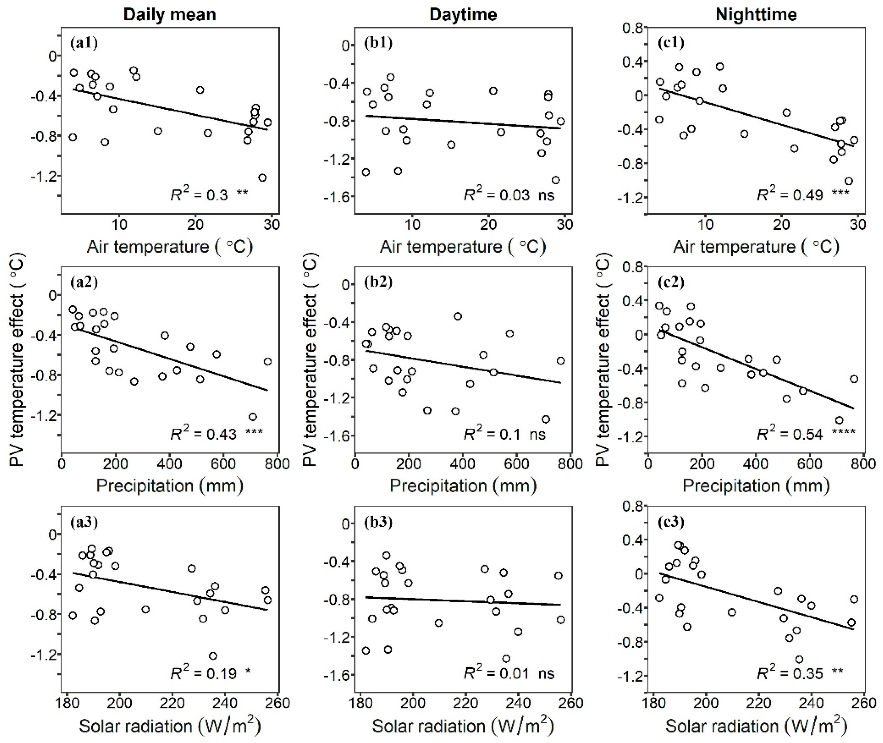
3.2. The PV Temperature Effect Varied with Geographical and Climatic Conditions

Given that the PV powerplants are distributed in different geographical and climate regions and numerous factors could affect the PV temperature effect, we used the conventional meteorological and geographical factors to examine if the PV temperature effect of the PV powerplants were related to these factors. For geographical factors, we found that the PV temperature effect of the daily mean surface temperature was significantly and positively correlated with latitude (p < 0.001) (Figure 3(a2)), but insignificantly correlated with longitude and altitude (p > 0.05) (Figure 3(a1,3)). We further examined the PV temperature effect during the daytime and nighttime separately and found that the positive correlations of PV temperature effect with latitude and altitude were both statistically significant (p < 0.05) (Figure 3(c2,3)) during the nighttime, but not the daytime (p > 0.05) (Figure 3(b2,3)).
For climate factors, we found that the PV effect on the daily mean surface temperature was negatively correlated with local annual mean air temperature, precipitation, and solar radiation (p < 0.05) (Figure 4(a1–3)). We further examined the PV temperature effect during the daytime and nighttime separately and found that the above-mentioned correlations were statistically significant (p < 0.01) only during the nighttime (Figure 4(c1–3)), but not the daytime (p > 0.05) (Figure 4(b1–3)). In addition, we found some PV powerplants even had warming effects during nighttime in a dry and cold environment (Figure 4(c1,2)).

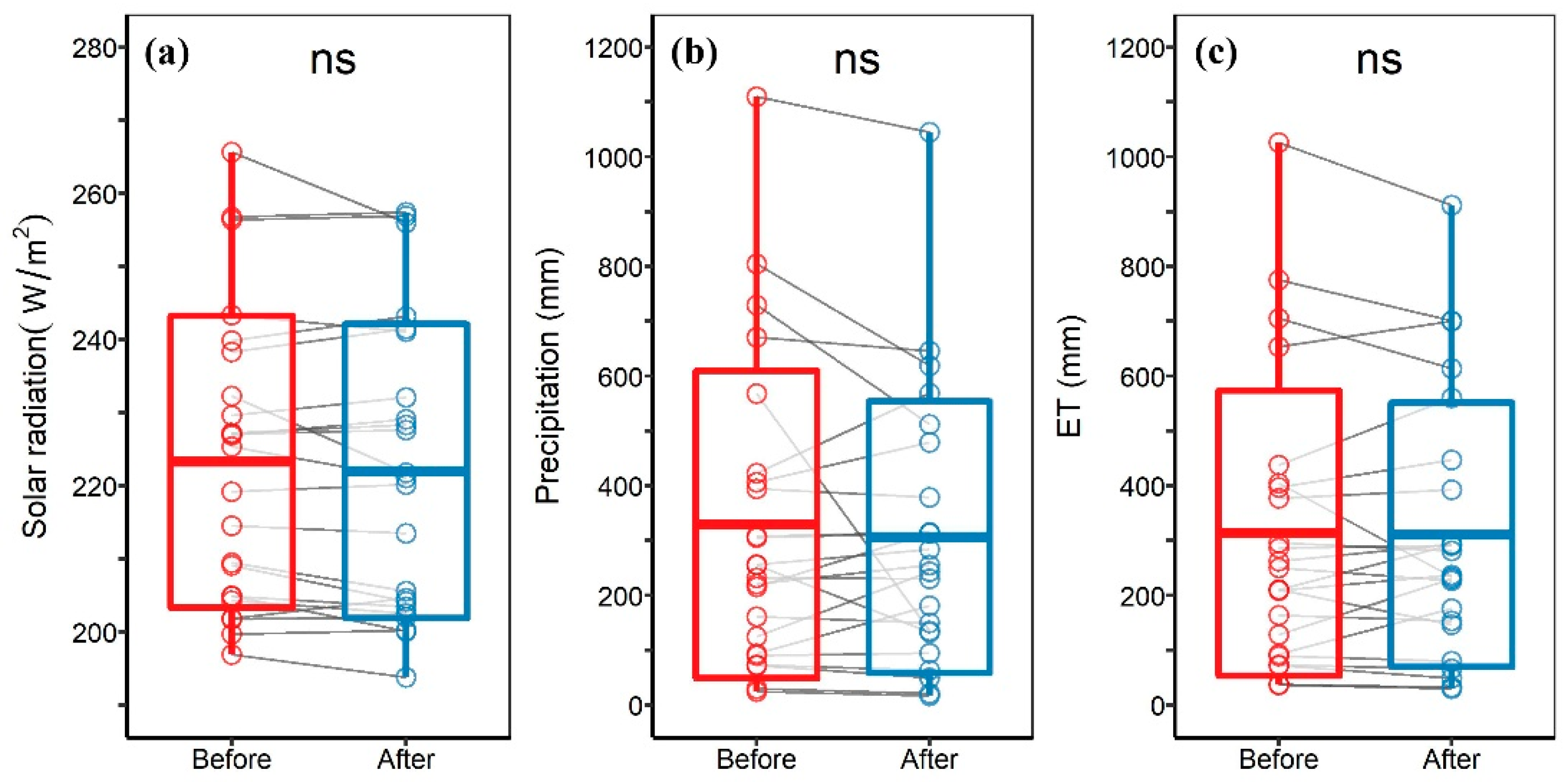
3.3. Impacts of Surface Conditions on the PV Temperature Effect

We compared the PV temperature effect with the site surface condition, such as vegetation cover and surface albedo, and found that the PV temperature effect on daily mean surface temperature was negatively correlated with vegetation cover (p < 0.01), namely NDVI (Figure 5(a1)), suggesting the cooling effect was strengthened under a better vegetation cover on the background. Similar to the climate variables, we also found that the correlations were statistically significant only during nighttime (p < 0.001) (Figure 5(c1)), but not the daytime (p > 0.05) (Figure 5(b1)). However, we found that the albedo had little relationship with the PV temperature effect, regardless of daily mean, daytime, or nighttime temperature (p > 0.05) (Figure 5(a2,b2,c2)).

3.4. Modelling the PV Temperature Effect

We further built multiple regression models to predict the PV temperature effect. The models are driven by climate, surface albedo, and scale of the PV powerplants. For the PV temperature effect we used the average temperature change (difference after and before the installation of the powerplant, Y1 in Equation (2), °C), temperature change per unit land area (Y2 in Equation (3), °C/km2), and temperature change per unit of potential annual electricity production which was calculated by multiplying the powerplant area, installation capacity per unit land area, and the potential electricity production per installation capacity (°C/KWh, Y3 in Equation (4)). We found that the multiple regression models can be used to predict the PV temperature effect very well with the coefficient of determinant (R2) of 0.94, 0.96, and 0.96 for models Y1, Y2, and Y3, respectively. The models are listed as:
Y 1 = a 0 + a 1 T a + a 2 P + a 3 P 2 + a 4 R s + a 5 R s 2 + a 6 V p + a 7 V p 2 + a 8 W s + a 9 W s 2 + a 10 α 1 + a 11 α 2 + a 12 α 2 2 + α 13 A    ( R 2 = 0.94 ,   Adjusted   R 2 = 0.85 ,   p   <   0.001 )
Y 2 = b 0 + b 1 T a + b 2 P + b 3 P 2 + b 4 R s + b 5 R s 2 + b 6 V p + b 7 V p 2 + b 8 W s + b 9 W s 2 + b 10 α 1 + b 11 α 2 + b 12 α 2 2       ( R 2 = 0.96 ,   Adjusted   R 2 = 0.91 ,   p   <   0.001 )
Y 3 = c 0 + c 1 T a + c 2 P + c 3 P 2 + c 4 R s + c 5 R s 2 + c 6 V p + c 7 V p 2 + c 8 W s + c 9 W s 2 + c 10 α 1 + c 11 α 2 + c 12 α 2 2       ( R 2 = 0.96 ,   Adjusted   R 2 = 0.91 ,   p   <   0.001 )
where Y1, Y2, and Y3 are PVPPTE (°C), PVPPTE/A (°C/km2), and PVPPTE/(A·PVOUT·D) (°C/KWh), respectively; Ta is air temperature (°C), P is precipitation (mm), Rs is solar radiation (W/m2), Vp is vapor pressure (kPa), Ws is wind speed (m/s), A is area of PV powerplant (km2), α1 is albedo before PV installation, α2 is albedo after PV installation and PVOUT is potential PV electricity production per unit capacity (KWh/KWp per year); D is the installed capacity density, which is 50,000 KW/km2 [43]. The parameters of the three models are listed in the Table 4, where ai, bi, and ci are the parameters for Equations (1), (2), and (3), respectively.

4. Discussion

4.1. Uncertainties in MODIS Surface Temperature and Emissivity

The MODIS is equipped with a cross-track scanning and covers a vast swath of 2330 kilometers in width in the east–west direction, yielding view angle of up to ±65 degrees (a negative value means viewing the grid from east) and a view time (local time) difference of up to about two hours in one scene [57]. Different viewing angle and time could cause the difference in radiative transfer length in the atmospheric profiles, the directional emissivity of heterogeneous surface, and even the pixel size, which could compromise the accuracy of the derived LST [45,58,59,60]. In this study, the method we used could minimize the viewing angle and time effects. First, we used the MOD11/MYD11 LST products to calculate the relative surface temperature (∆surface temperature) between the PV powerplant and its control area (buffer area) and the temperature before and after the installation of each PV powerplant to quantify the PV temperature effect. The atmospheric condition, view time, and view angle over the PV powerplant and its control area should be the same or almost the same because the powerplant and its control area are adjacent to each other and normally within a few kilometers in the east–west direction. Second, though the view times and view angles of different pixels in the east–west direction could be quite different on the same MODIS LST scene, the annual mean view angles and view times (local time) of different locations are quite similar because the MODIS orbits shift to minimize the view angle and view time effects (Figures S1 and S2). In the current study we used the annual mean surface temperature which was calculated based on hundreds of clear-sky observations in one year. We found that the annual mean view angles in non-polar regions were very similar with a difference of merely a few degrees (Figure S1). In the middle and low latitudes of the northern hemisphere (0–45°) where most of our PV power stations are located, the difference of annual mean view time from Terra is within 30 minutes (Figure S2). Finally, in case of view angle and view time biases, our normalization approach by using a surrounding buffer as reference for each powerplant will eliminate the associated errors.
It is well known that the satellite measured surface temperature is very sensitive to surface emissivity [61]. In the current study we are more concerned about the change of emissivity with the construction of the PV powerplants because a fixed emissivity value was used for each landcover type in the MODIS algorithm (Table S1). The MODIS surface temperature was computed based on the constant emissivity value for each of the 18 landcover type [62,63]. Apparently, there is no such a landcover type of “PV powerplant” in the MODIS emissivity classification. The change of emissivity mainly comes from the difference of emissivity between the background soil and the PV panel because the vegetation cover is very low in most of the PV powerplants. The PV panels are usually coated with a glass layer and thus the emissivity of the PV panels is mostly determined by this glass layer. We find that the emissivity of the PV panels with glass coating is very close to or, in some cases, slightly lower than those of sandy soils and dry vegetations which are commonly seen in the PV powerplant areas [64,65,66,67] (Table S2). It is noted that the collective emissivity of the PV panels in a powerplant should be greater than that of individual PV panels because of the cavity effect [68,69,70]. Using a method recently published in the literature [68], we calculated the cavity effect on emissivity in the PV powerplants (Appendix A) and found the cavity effect would increase the emissivity of the PV panels with an average increase of 0.005 (Table S3). By including the cavity effect, the collective emissivity of the PV panels almost perfectly matched those of the background sandy soils. The construction of the PV powerplant is detrimental to vegetation in the first few years but then beneficial to vegetation growth because the panel shading suppresses evaporation and thus improves soil moisture which further promotes vegetation growth [71]. As a result, the construction of PV powerplants had little impact on vegetation which usually covered a small portion of the land surface. Our results also confirmed that the average NDVI over the 23 PV powerplants had barely changed after the installation of the powerplants (Figure 6b). Therefore, it is reasonable to believe that the emissivity did not significantly change with the construction of the PV powerplants. At present, direct measurements of emissivity over the PV powerplants are lacking but are timely needed to improve the accuracy of remote sensing-based measurements of surface temperature.

4.2. Effects of Albedo and Electrical Energy Conversion on Surface Temperature

By comparing the surface temperature changes of the 23 largest PV powerplants in the world, we found that the installation of the PV powerplants significantly reduced the surface temperature in the powerplants. It is commonly believed that installation of PV panels will change surface reflectance of solar radiation and thus change the surface energy budgets, which could result in surface cooling. In the current study we found that the average albedo significantly decreased from 0.22 to 0.184 with the installation of the PV powerplants (Figure 6a). The albedo may be affected by two factors. Disturbances of vegetation and soils, such as soil compactness, due to the construction and operation of the powerplants will often increase surface albedo. In contrast, the installation of solar panels will decrease surface albedo because the albedo of PV panels typically ranges from 0.06 to 0.1 with an average of about 0.08 which is much lower than the background albedo of about 0.22 [6]. Our result that albedo decreased with the installation of powerplants suggests that the solar panel effect exceeds the disturbance effect. However, albedo alone cannot explain the decrease of surface temperature because lowering albedo means the surface will receive more solar energy and thus increase surface temperature if the incoming solar radiation does not change. Indeed, we found that the incoming solar radiation barely changed before and after the installation of the PV powerplants using the high-resolution ERA reanalysis climate data (Figure 7a).
PV panels can normally convert 10% to 15% of the absorbed solar energy to electricity exported to the grid, which tends to make the surface cooler [6]. The effective albedo, albedo corrected with electricity conversion [6], should be much higher. We obtained an average effective albedo of 0.244 with PV powerplants albedo of 0.184 and assuming an electricity conversion efficiency of 0.12 [6] and a spacing factor of 0.5 [72,73]. This effective albedo is significantly greater than the pre-construction albedo of 0.22 (p < 0.01). Therefore, we conclude that the electricity conversion effect has contributed the most to the observed surface cooling. However, the albedo and electricity conversion effects cannot explain the observed surface cooling during nighttime because solar radiation, albedo, and electricity generation do not exist at all during the nighttime.

4.3. Solar Panel Shading and Evapotranspiration Cooling Effects on Surface Temperature

In addition to albedo, evapotranspiration (ET) could also change surface temperature through the partition of surface energy balance. Precipitation and vegetation conditions are the key factors in determining local ET. In many ecosystems ET is dominated by plant transpiration even in the areas with low vegetation cover [74]. Most of the PV powerplants are located in arid and semi-arid areas as evidenced by the precipitation data in Table 2. Previous studies have shown that PV powerplants may have enhanced or little impact on the plant growth due mainly to the shading effect where the shades of the PV panels cool the vegetation and soils during the daytime [71,75]. Our results confirmed that the PV powerplants had little impact on vegetation as evidenced by the minimal reduction in NDVI after the construction of the powerplants (Figure 6b). Furthermore, we found that the precipitation and ET over the powerplants and their surroundings rarely changed with the construction of powerplants (Figure 7b,c). Therefore, we think that ET had little contribution to the observed surface cooling while the solar panels might have cooled the soil and vegetation surfaces through the shading effect (Figure S3, Table S4). Again, this shading effect cannot explain the observed nighttime surface cooling in the PV powerplants.

4.4. Convective Cooling Effect on Surface Temperature of Solar Panels

Most of the PV powerplants had low vegetation, usually covered by grasses or short shrubs. The installation of the powerplants will increase the surface roughness and change the wind profile [20]. The low heat capacity and high thermal conductivity of the PV panels as compared with those of soils make their temperature change more rapidly. The PV panels often stand about 1–2 m above the ground and act as a “heater” in the air during the daytime by absorbing solar radiation [20,21,22,23]. Solar panels are more effective in heating the air than the normal ground surfaces (soils and vegetation) for two reasons. First, solar panels can exchange heat with the air on both upper and lower surfaces. Second, stronger turbulence around the solar panels can also promote heat exchange with the air due to a greater wind speed in the air than at the ground surface. It is through this convection process that more heat is transferred from the panels to the air, making the solar panels relatively cooler and the ambient air warmer. We think that this convective cooling also made a considerable contribution to the observed surface cooling in the PV powerplants. Previous studies have reported that PV powerplants have increased air temperature in various regions [20,21,22], and a recent study also declared that PV powerplant could decrease the land surface temperature [43].
The nighttime cooling effect of the PV powerplants is not independent of its daytime cooling. Each solar panel in the powerplants plays a role as electricity convertor and convective heater during the daytime by transferring energy into electricity and sensible heat into the air. As a result, less solar energy can reach the ground. The reduction of ground energy input will further reduce the nighttime surface temperature. Additionally, the night surface temperature in PV modules decrease faster than the natural surface by radiation and thermal diffusion with the lower heat capacity and higher thermal conduction of the PV modules than those of the natural surface [20,76]. Our findings that PV powerplants can reduce the surface temperature in both daytime and nighttime are important for better understanding the climate and environmental impacts of PV powerplants which are under rapid construction worldwide.

4.5. Association of the PV Temperature Effect with Geographic, Climatic, and Vegetation Factors

In addition to reporting the surface cooling phenomena of the PV powerplants, we further examined if the surface cooling effect varies with geographic, climatic, and vegetation factors. Firstly, we found that the PV temperature effect was significantly correlated with latitude but not longitude and altitude (Figure 3), suggesting the PV temperature effect was different in different geographic regions. This finding is useful for site selection of new PV powerplants by including the direct climate effect, the cooling effect on surface temperature, of the PV powerplants. Currently, most of the PV powerplants are located in the mid- and high-latitude regions due partly to maximizing electricity production. In the future, more PV powerplants may be constructed in the lower latitudes, such as the semi-arid regions in the tropics and subtropics, to achieve the goal of clean electricity as well as direct climate benefits. However, the geographic variables are insufficient to explain the mechanism of the observed latitudinal gradient of the PV temperature effect. It is well known that latitude is a composite indicator of soil, vegetation, and climate, such as solar radiation, temperature, and precipitation.
In this study we also examined the correlation between the PV temperature effect and climate and found that the temperature effect was highly and negatively correlated with temperature, precipitation, and solar radiation. The lower latitudes generally have greater annual mean temperature, precipitation, and solar radiation which favor plant growth (Table 1 and Table 2). This is confirmed by the greater NDVI values in the lower latitudes before the construction of the PV powerplants (Figure 8a). Thus, the lower latitudes also saw a greater reduction in vegetation cover due to the construction of the PV powerplants (Figure 8b). The reduction of vegetation cover rendered the surface cooling during night because vegetation had a greater water content than the dry soils and thus vegetation acted as thermal inertia. The lack of correlation between the PV daytime temperature effect and latitude, climate, and NDVI (Figure 3, Figure 4 and Figure 5) can also be explained by the greater reduction of vegetation cover in the lower latitudes (Figure 8b). This is because the transpiration cooling effect was weakened relatively more in the warmer, wetter, and sunnier areas in the lower latitudes. In addition, the greater PV nighttime cooling effect with increasing precipitation (Figure 3(c2)) suggests that the PV modules which have a high thermal conductivity and act as a radiator during nighttime are more effective in dissipating the thermal energy stored in the wetter soils. To our surprise, we did not find any correlation between the PV temperature effect and surface albedo which is critical to surface energy balance (Figure 5(a2,b2,c2)). This is because albedo is determined by many factors, such as soil, vegetation, color, roughness, and moisture content, and its effect on temperature might be cancelled out by other processes. For instance, increasing soil moisture will decrease albedo and thus make the surface warmer. Meanwhile, increasing soil moisture will also enhance evapotranspiration which makes the surface cooler. In addition, we found that the scale and capacity of the PV powerplants could also affect the PV temperature effect with greater cooling in larger powerplants in terms of area and potential capacity (Equations (2)–(4), Table 1 and Table 3). In summary, the PV powerplants took their effect on local surface temperature mainly through their impacts on surface energy budgets and water cycle through vegetation which is also determined by the regional climate. Our regression analyses provide some preliminary insights on the complex interactions among the PV panel, soil, and vegetation through energy flow, water cycle, and climate regulation. We think remote sensing alone is insufficient to elucidate this complex issue. More studies are needed to reveal the mechanisms of the impacts of various PV powerplants on the local and regional climate through experimental and modeling approaches. Nevertheless, the PV temperature effect can be well predicted by climate, surface albedo, and scale of the powerplants, such as area and potential electricity production, with more than 94% of the variance of the PV temperature effect explained by those variables (Equations (2)–(4)). The area and capacity-based PV cooling effects can be modeled even better with those variables. These results can be used to estimate the direct climate effect of the PV powerplants with smaller scales (area or capacity), a useful information guiding the planning, designing, and site selecting for constructing new PV powerplants.

5. Conclusions

In this study, we assessed the effects of PV powerplants on surface temperature with 23 largest PV powerplants in the world based on the MODIS thermal band dataset. We found that the installation of PV powerplants had reduced the daily mean surface temperature at a statistically significant level in the PV powerplant areas. We also found that the powerplant cooling effect was evidenced in both daytime and nighttime, but the daytime cooing was much stronger than the nighttime. This cooling effect was also depended on the capacity of the powerplants with a cooling rate of −0.32, −0.48, and −0.14 °C/TWh, respectively, for daily mean, daytime, and nighttime temperature. Unexpectedly, the PV powerplants had little effect on vegetation growth as indicated by the slightly decrease in NDVI. Our further analyses showed that the cooling effect of the powerplants was mainly attributed to the enhanced effective albedo, solar panel shading, and convection cooling of the solar panels.
Our results highlight the effect of PV powerplants on surface temperature, which will not only improve our understanding on the climate effects of PV powerplants but also provide important information in guiding the selection of PV powerplant sites in different geographical and climate regions. For example, constructing more PV powerplants in the lower latitudes may have a greater cooling effect on surface temperature. The current study also provides an effective method to further investigate the effect of the PV powerplants on temperature with the increasing installation of large-scale PV powerplants and rapid development in thermal remote sensing techniques.

Supplementary Materials

The following are available online at https://www.mdpi.com/2072-4292/12/11/1825/s1, Figure S1: The annual mean view angle from MODIS Terra during daytime in 2018. Figure S2: The annual mean view time from MODIS Terra during daytime in 2018. Figure S3: Diagrammatic sketch of PV panels. The α is tilt angle of PV panel, which is equal to the latitude of the PV powerplant [77], and the β is solar altitude angle (SAA). Table S1: The emissivity values used for the MODIS LST products (band 31 and 32) based on the classification-based emissivity model. Table S2: Comparison of the emissivity of the sands, dry vegetation and PV solar cells. Table S3: The cavity effect of the PV panels in different PV power stations. Table S4: The solar altitude angle (SAA) and proportion of shade surface of each powerplant at the MODIS passing time during daytime (10:30 local time) on June Solstice, September Equinox and December Solstice. The solar altitude angle at 13:30 (local time) is equal to the solar altitude angle at 10:30 (local time). Tilt angle is equal to the latitude of the PV powerplant.

Author Contributions

Conceptualization, X.Z. and M.X.; methodology, X.Z. and M.X.; software, X.Z.; validation, X.Z.; writing—original draft preparation, X.Z.; writing—review and editing, M.X.; visualization, X.Z.; supervision, M.X.; funding acquisition, M.X. All authors have read and agreed to the published version of the manuscript.

Funding

This study was supported by the National Key Research and Development Program of China (2018YFA0606500, 2017YFA0604302).

Acknowledgments

We appreciate Mojtaba Zeraatpisheh, Hua Shang and Ruolan Li for their help with the writing of this paper. We also thank Steven Xu for his help polish the English language of the manuscript.

Conflicts of Interest

The authors declare no conflict of interest.

Appendix A. Cavity Effect of the PV Powerplants

The cavity effect of PV panels is the internal reflections of electromagnetic waves among the PV panels at each PV powerplant. In this study, we used the same model as in Yamamoto and Ishikawa (2018) by treating the PV panels as an infinitely Lambertian box in the east–west direction [68], which means no cavity effect in the east–west direction because all the PV panels were installed facing the south. In the north–south direction along the satellite flight path the satellite view angle θ is assumed about zero because the satellite is passing the PV powerplant overhead. The cavity effect of the PV panels was estimated as:
d ε = ( 1 ε g ) ε s [ ( 1 + H / S ) 1 + ( H / S ) 2 ] P g
where H is the average height of PV panels, S is the distance of ground, L is the projection distance of PV panels in north–south direction, εg is the emissivity of ground, εs is emissivity of PV panels and Pg is the ground proportion observed by the sensor. In our study, the S is equal to L, the H is equal to 0.5·tanα·L, where α is tilt angle of PV panels, and Pg is equal to 0.5 (Figure S3). The result of the cavity effect of the PV powerplants is shown in Table S3.

References

  1. Johansson, T.B.; Patwardhan, A.P.; Nakićenović, N.; Gomez-Echeverri, L. Global Energy Assessment: Toward a Sustainable Future; Cambridge University Press: Cambridge, UK, 2012. [Google Scholar]
  2. Nemet, G.F. Net radiative forcing from widespread deployment of photovoltaics. Environ. Sci. Technol. 2009, 43, 2173–2178. [Google Scholar] [CrossRef]
  3. Akella, A.; Saini, R.; Sharma, M.P. Social, economical and environmental impacts of renewable energy systems. Renew. Energy 2009, 34, 390–396. [Google Scholar] [CrossRef]
  4. Muneer, T.; Asif, M.; Kubie, J. Generation and transmission prospects for solar electricity: UK and global markets. Energy Convers. Manag. 2003, 44, 35–52. [Google Scholar] [CrossRef]
  5. Zou, H.; Du, H.; Brown, M.A.; Mao, G. Large-scale PV power generation in China: A grid parity and techno-economic analysis. Energy 2017, 134, 256–268. [Google Scholar] [CrossRef]
  6. Taha, H. The potential for air-temperature impact from large-scale deployment of solar photovoltaic arrays in urban areas. Solar Energy 2013, 91, 358–367. [Google Scholar] [CrossRef]
  7. Hernandez, R.R.; Easter, S.; Murphy-Mariscal, M.L.; Maestre, F.T.; Tavassoli, M.; Allen, E.B.; Barrows, C.W.; Belnap, J.; Ochoa-Hueso, R.; Ravi, S. Environmental impacts of utility-scale solar energy. Renew. Sust. Energy Rev. 2014, 29, 766–779. [Google Scholar] [CrossRef] [Green Version]
  8. Zhai, P.; Larsen, P.; Millstein, D.; Menon, S.; Masanet, E. The potential for avoided emissions from photovoltaic electricity in the United States. Energy 2012, 47, 443–450. [Google Scholar] [CrossRef] [Green Version]
  9. Duan, H.-B.; Zhang, G.-P.; Zhu, L.; Fan, Y.; Wang, S.-Y. How will diffusion of PV solar contribute to China’s emissions-peaking and climate responses? Renew. Sust. Energy Rev. 2016, 53, 1076–1085. [Google Scholar] [CrossRef]
  10. Aliprandi, F.; Stoppato, A.; Mirandola, A. Estimating CO2 emissions reduction from renewable energy use in Italy. Renew. Energy 2016, 96, 220–232. [Google Scholar] [CrossRef]
  11. Krauter, S.; Rüther, R. Considerations for the calculation of greenhouse gas reduction by photovoltaic solar energy. Renew. Energy 2004, 29, 345–355. [Google Scholar] [CrossRef]
  12. Peng, J.; Lu, L.; Yang, H. Review on life cycle assessment of energy payback and greenhouse gas emission of solar photovoltaic systems. Renew. Sust. Energ. Rev. 2013, 19, 255–274. [Google Scholar] [CrossRef]
  13. Battisti, R.; Corrado, A. Evaluation of technical improvements of photovoltaic systems through life cycle assessment methodology. Energy 2005, 30, 952–967. [Google Scholar] [CrossRef]
  14. Dones, R.; Frischknecht, R. Life-cycle assessment of photovoltaic systems: Results of Swiss studies on energy chains. Prog. Photovolt. 1998, 6, 117–125. [Google Scholar] [CrossRef]
  15. Salamanca, F.; Georgescu, M.; Mahalov, A.; Moustaoui, M.; Martilli, A. Citywide impacts of cool roof and rooftop solar photovoltaic deployment on near-surface air temperature and cooling energy demand. Bound. Layer Meteorol. 2016, 161, 203–221. [Google Scholar] [CrossRef] [Green Version]
  16. Masson, V.; Bonhomme, M.; Salagnac, J.-L.; Briottet, X.; Lemonsu, A. Solar panels reduce both global warming and urban heat island. Front. Environ. Sci. 2014, 2, 14. [Google Scholar] [CrossRef]
  17. Hu, A.; Levis, S.; Meehl, G.A.; Han, W.; Washington, W.M.; Oleson, K.W.; van Ruijven, B.J.; He, M.; Strand, W.G. Impact of solar panels on global climate. Nat. Clim. Change. 2016, 6, 290. [Google Scholar] [CrossRef]
  18. Millstein, D.; Menon, S. Regional climate consequences of large-scale cool roof and photovoltaic array deployment. Environ. Res. 2011, 6, 034001. [Google Scholar] [CrossRef]
  19. Li, Y.; Kalnay, E.; Motesharrei, S.; Rivas, J.; Kucharski, F.; Kirk-Davidoff, D.; Bach, E.; Zeng, N. Climate model shows large-scale wind and solar farms in the Sahara increase rain and vegetation. Science 2018, 361, 1019–1022. [Google Scholar] [CrossRef] [Green Version]
  20. Broadbent, A.M.; Krayenhoff, E.S.; Georgescu, M.; Sailor, D.J. The observed effects of utility-scale photovoltaics on near-surface air temperature and energy balance. J. Appl. Meteorol. Climatol. 2019, 58, 989–1006. [Google Scholar] [CrossRef]
  21. Yang, L.; Gao, X.; Lv, F.; Hui, X.; Ma, L.; Hou, X. Study on the local climatic effects of large photovoltaic solar farms in desert areas. Solar Energy 2017, 144, 244–253. [Google Scholar] [CrossRef]
  22. Barron-Gafford, G.A.; Minor, R.L.; Allen, N.A.; Cronin, A.D.; Brooks, A.E.; Pavao-Zuckerman, M.A. The photovoltaic heat island effect: Larger solar power plants increase local temperatures. Sci. Rep. 2016, 6, 35070. [Google Scholar] [CrossRef] [PubMed] [Green Version]
  23. Chang, R.; Shen, Y.; Luo, Y.; Wang, B.; Yang, Z.; Guo, P. Observed surface radiation and temperature impacts from the large-scale deployment of photovoltaics in the barren area of Gonghe, China. Renew. Energy 2018, 118, 131–137. [Google Scholar] [CrossRef]
  24. Fu, G.; Shen, Z.; Zhang, X.; Shi, P.; Zhang, Y.; Wu, J. Estimating air temperature of an alpine meadow on the northern Tibetan Plateau using MODIS land surface temperature. Acta Ecol. Sinica 2011, 31, 8–13. [Google Scholar] [CrossRef]
  25. Vancutsem, C.; Ceccato, P.; Dinku, T.; Connor, S.J. Evaluation of MODIS land surface temperature data to estimate air temperature in different ecosystems over Africa. Remote Sens. Environ. 2010, 114, 449–465. [Google Scholar] [CrossRef]
  26. Shamir, E.; Georgakakos, K.P. MODIS Land surface temperature as an index of surface air temperature for operational snowpack estimation. Remote Sens. Environ. 2014, 152, 83–98. [Google Scholar] [CrossRef]
  27. Zhu, W.; Lű, A.; Jia, S. Estimation of daily maximum and minimum air temperature using MODIS land surface temperature products. Remote Sens. Environ. 2013, 130, 62–73. [Google Scholar] [CrossRef]
  28. Zhu, W.; Lű, A.; Jia, S.; Yan, J.; Mahmood, R. Retrievals of all-weather daytime air temperature from MODIS products. Remote Sens. Environ. 2017, 189, 152–163. [Google Scholar] [CrossRef]
  29. Luo, D.; Jin, H.; Marchenko, S.S.; Romanovsky, V.E. Difference between near-surface air, land surface and ground surface temperatures and their influences on the frozen ground on the Qinghai-Tibet Plateau. Geoderma 2018, 312, 74–85. [Google Scholar] [CrossRef]
  30. Justice, C.; Townshend, J.; Vermote, E.; Masuoka, E.; Wolfe, R.; Saleous, N.; Roy, D.; Morisette, J. An overview of MODIS Land data processing and product status. Remote Sens. Environ. 2002, 83, 3–15. [Google Scholar] [CrossRef]
  31. Peng, S.; Piao, S.; Ciais, P.; Friedlingstein, P.; Ottle, C.; Bréon, F.o.-M.; Nan, H.; Zhou, L.; Myneni, R.B. Surface urban heat island across 419 global big cities. Environ. Sci. Technol. 2011, 46, 696–703. [Google Scholar] [CrossRef]
  32. Lazzarini, M.; Marpu, P.R.; Ghedira, H. Temperature-land cover interactions: The inversion of urban heat island phenomenon in desert city areas. Remote Sens. Environ. 2013, 130, 136–152. [Google Scholar] [CrossRef]
  33. Neteler, M. Estimating daily land surface temperatures in mountainous environments by reconstructed MODIS LST data. Remote Sens. 2010, 2, 333–351. [Google Scholar] [CrossRef] [Green Version]
  34. Anderson, M.C.; Allen, R.G.; Morse, A.; Kustas, W.P. Use of Landsat thermal imagery in monitoring evapotranspiration and managing water resources. Remote Sens. Environ. 2012, 122, 50–65. [Google Scholar] [CrossRef]
  35. Westermann, S.; Langer, M.; Boike, J. Spatial and temporal variations of summer surface temperatures of high-arctic tundra on Svalbard—Implications for MODIS LST based permafrost monitoring. Remote Sens. Environ. 2011, 115, 908–922. [Google Scholar] [CrossRef]
  36. Dousset, B.; Gourmelon, F. Satellite multi-sensor data analysis of urban surface temperatures and landcover. Int. J. Photogramm. Remote Sens. 2003, 58, 43–54. [Google Scholar] [CrossRef]
  37. Guangmeng, G.; Mei, Z. Using MODIS land surface temperature to evaluate forest fire risk of northeast China. IEEE Geosci. Remote Sens. Lett. 2004, 1, 98–100. [Google Scholar] [CrossRef]
  38. Imhoff, M.L.; Zhang, P.; Wolfe, R.E.; Bounoua, L. Remote sensing of the urban heat island effect across biomes in the continental USA. Remote Sens. Environ. 2010, 114, 504–513. [Google Scholar] [CrossRef] [Green Version]
  39. Weng, Q.; Lu, D.; Schubring, J. Estimation of land surface temperature-vegetation abundance relationship for urban heat island studies. Remote Sens. Environ. 2004, 89, 467–483. [Google Scholar] [CrossRef]
  40. Wan, Z. New refinements and validation of the collection-6 MODIS land-surface temperature/emissivity product. Remote Sens. Environ. 2014, 140, 36–45. [Google Scholar] [CrossRef]
  41. Gorelick, N.; Hancher, M.; Dixon, M.; Ilyushchenko, S.; Thau, D.; Moore, R. Google earth engine: Planetary-scale geospatial analysis for everyone. Remote Sens. Environ. 2017, 202, 18–27. [Google Scholar] [CrossRef]
  42. Global Solar Atlas 2.0, a Free, Web-Based Application is Developed and Operated by the Company Solargis S.R.O. on Behalf of the World Bank Group, Utilizing Solargis Data, with Funding Provided by the Energy Sector Management Assistance Program (ESMAP). Available online: https://globalsolaratlas.info (accessed on 17 May 2020).
  43. Chang, R.; Luo, Y.; Zhu, R. Simulated local climatic impacts of large-scale photovoltaics over the barren area of Qinghai, China. Renew. Energy 2020, 145, 478–489. [Google Scholar] [CrossRef]
  44. Wang, K.; Wan, Z.; Wang, P.; Sparrow, M.; Liu, J.; Haginoya, S. Evaluation and improvement of the MODIS land surface temperature/emissivity products using ground-based measurements at a semi-desert site on the western Tibetan Plateau. Int. J. Remote Sens. 2007, 28, 2549–2565. [Google Scholar] [CrossRef]
  45. Wan, Z.; Dozier, J. A generalized split-window algorithm for retrieving land-surface temperature from space. IEEE Trans. Geosci. Remote Sens. 1996, 34, 892–905. [Google Scholar]
  46. Wan, Z. Estimate of noise and systematic error in early thermal infrared data of the moderate resolution imaging spectroradiometer (MODIS). Remote Sens. Environ. 2002, 80, 47–54. [Google Scholar] [CrossRef]
  47. Wan, Z. MODIS Land Surface Temperature Products Users’ Guide; Institute for Computational Earth System Science: Santa Barbara, CA, USA, 2006. [Google Scholar]
  48. Homer, N.; Merriman, B.; Nelson, S.F. BFAST: An alignment tool for large scale genome resequencing. PLoS ONE 2009, 4, e7767. [Google Scholar] [CrossRef] [Green Version]
  49. Rouse, J.W., Jr.; Haas, R.; Schell, J.; Deering, D. Monitoring vegetation systems in the great plains with ERTS. NASAS 1974, 351, 309. [Google Scholar]
  50. Huete, A.; Didan, K.; Miura, T.; Rodriguez, E.P.; Gao, X.; Ferreira, L.G. Overview of the radiometric and biophysical performance of the MODIS vegetation indices. Remote Sens. Environ. 2002, 83, 195–213. [Google Scholar] [CrossRef]
  51. Li, Y.; Zhao, M.; Motesharrei, S.; Mu, Q.; Kalnay, E.; Li, S. Local cooling and warming effects of forests based on satellite observations. Nat. Commun. 2015, 6, 6603. [Google Scholar] [CrossRef] [Green Version]
  52. Fick, S.E.; Hijmans, R.J. WorldClim 2: New 1-km spatial resolution climate surfaces for global land areas. Int. J. Climatol. 2017, 37, 4302–4315. [Google Scholar] [CrossRef]
  53. Panagos, P.; Ballabio, C.; Meusburger, K.; Spinoni, J.; Alewell, C.; Borrelli, P. Towards estimates of future rainfall erosivity in Europe based on REDES and WorldClim datasets. J. Hydrol. 2017, 548, 251–262. [Google Scholar] [CrossRef]
  54. Beck, H.E.; Vergopolan, N.; Pan, M.; Levizzani, V.; van Dijk, A.I.J.M.; Weedon, G.P.; Brocca, L.; Pappenberger, F.; Huffman, G.J.; Wood, E.F. Global-scale evaluation of 22 precipitation datasets using gauge observations and hydrological modeling. Hydrol. Earth Syst. Sci. 2017, 21, 6201–6217. [Google Scholar] [CrossRef] [Green Version]
  55. Beck, H.E.; Zimmermann, N.E.; McVicar, T.R.; Vergopolan, N.; Berg, A.; Wood, E.F. Present and future Köppen-Geiger climate classification maps at 1-km resolution. Sci. Data 2018, 5, 180214. [Google Scholar] [CrossRef] [PubMed] [Green Version]
  56. Hersbach, H.; Dee, D. ERA5 reanalysis is in production. ECMWF Newsletter 2016, 147, 5–6. [Google Scholar]
  57. Barnes, W.L.; Pagano, T.S.; Salomonson, V.V. Prelaunch characteristics of the moderate resolution imaging spectroradiometer (MODIS) on EOS-AM1. IEEE Trans. Geosci. Remote Sens. 1998, 36, 1088–1100. [Google Scholar] [CrossRef] [Green Version]
  58. Li, Z.-L.; Tang, B.-H.; Wu, H.; Ren, H.; Yan, G.; Wan, Z.; Trigo, I.F.; Sobrino, J.A. Satellite-derived land surface temperature: Current status and perspectives. Remote Sens. Environ. 2013, 131, 14–37. [Google Scholar] [CrossRef] [Green Version]
  59. Sobrino, J.A.; Cuenca, J. Angular variation of thermal infrared emissivity for some natural surfaces from experimental measurements. Appl. Opt. 1999, 38, 3931–3936. [Google Scholar] [CrossRef]
  60. Ghent, D.; Veal, K.; Trent, T.; Dodd, E.; Sembhi, H.; Remedios, J. A new approach to defining uncertainties for MODIS land surface temperature. Remote Sens. 2019, 11, 1021. [Google Scholar] [CrossRef] [Green Version]
  61. Becker, F. The impact of spectral emissivity on the measurement of land surface temperature from a satellite. Int. J. Remote Sens. 1987, 8, 1509–1522. [Google Scholar] [CrossRef]
  62. Wan, Z. New refinements and validation of the MODIS land-surface temperature/emissivity products. Remote Sens. Environ. 2008, 112, 59–74. [Google Scholar] [CrossRef]
  63. Snyder, W.C.; Wan, Z.; Zhang, Y.; Feng, Y.-Z. Classification-based emissivity for land surface temperature measurement from space. Int. J. Remote Sens. 1998, 19, 2753–2774. [Google Scholar] [CrossRef]
  64. Hulley, G.C.; Hook, S.J. Intercomparison of versions 4, 4.1 and 5 of the MODIS land surface temperature and emissivity products and validation with laboratory measurements of sand samples from the Namib desert, Namibia. Remote Sens. Environ. 2009, 113, 1313–1318. [Google Scholar] [CrossRef]
  65. Rubio, E.; Caselles, V.; Badenas, C. Emissivity measurements of several soils and vegetation types in the 8–14 m wave band: Analysis of two field methods. Remote Sens. Environ. 1997, 59, 490–521. [Google Scholar] [CrossRef]
  66. Labuhn, D.; Kabelac, S. The spectral directional emissivity of photovoltaic surfaces. Int. J. Thermophys. 2001, 22, 1577–1592. [Google Scholar] [CrossRef]
  67. Thermography-A Quick Analysis. Available online: https://www.avisolar.com/post/thermography-quick-analysis (accessed on 15 April 2020).
  68. Yamamoto, Y.; Ishikawa, H. Thermal land surface emissivity for retrieving land surface temperature from Himawari-8. J. Meteorol. Soc. Jpn. Ser. II 2018, 96, 43–58. [Google Scholar] [CrossRef] [Green Version]
  69. Peres, L.F.; Dacamara, C.C. Emissivity maps to retrieve land-surface temperature from MSG/SEVIRI. IEEE Trans. Geosci. Remote Sens. 2005, 43, 1834–1844. [Google Scholar] [CrossRef]
  70. Caselles, V.; Sobrino, J. Determination of frosts in orange groves from NOAA-9 AVHRR data. Remote Sens. Environ. 1989, 29, 135–146. [Google Scholar] [CrossRef]
  71. Liu, Y.; Zhang, R.Q.; Huang, Z.; Cheng, Z.; López-Vicente, M.; Ma, X.R.; Wu, G.L. Solar photovoltaic panels significantly promote vegetation recovery by modifying the soil surface microhabitats in an arid sandy ecosystem. Land Degrad. Dev. 2019. [Google Scholar] [CrossRef]
  72. Araki, K.; Nagai, H.; Lee, K.-H.; Yamaguchi, M. Analysis of impact to optical environment of the land by flat-plate and array of tracking PV panels. Solar Energy 2017, 144, 278–285. [Google Scholar] [CrossRef]
  73. Kurokawa, K. Energy from the Desert: Feasibility of Very Large Scale Power Generation (VLS-PV) Systems; Routledge: Abingdon, UK, 2012. [Google Scholar]
  74. Jasechko, S.; Sharp, Z.D.; Gibson, J.J.; Birks, S.J.; Yi, Y.; Fawcett, P.J. Terrestrial water fluxes dominated by transpiration. Nature 2013, 496, 347. [Google Scholar] [CrossRef]
  75. Nghiem, J.; Potter, C.; Baiman, R. Detection of vegetation cover change in renewable energy development zones of southern california using MODIS NDVI time series analysis, 2000 to 2018. Environments 2019, 6, 40. [Google Scholar] [CrossRef] [Green Version]
  76. Armstrong, S.; Hurley, W.G. A thermal model for photovoltaic panels under varying atmospheric conditions. Appl. Therm. Eng. 2010, 30, 1488–1495. [Google Scholar] [CrossRef]
  77. Yadav, A.K.; Chandel, S.S. Tilt angle optimization to maximize incident solar radiation: A review. Renew. Sust. Energ. Rev. 2013, 23, 503–513. [Google Scholar] [CrossRef]
Figure 1. The time series (gray line) of the difference between the surface temperature in PV powerplant and the surface temperature in control region (surface temperature in PV powerplant minus surface temperature in control region, term as ∆surface temperature) during daytime from Zhongwei, China (105.03° E, 37.56° N), with 8-day data (gray line), trend (blue line), and abrupt change time (the dash vertical line) from 2003 to 2018. The PV temperature effect before the installation of the PV powerplants was calculated from the three years (one year starting with January and end with December) average surface temperature (green rectangle) before the abrupt change time and the PV temperature effect after installation of PV powerplants were calculated from the 2018-year average surface temperature.
Remotesensing 12 01825 g001
Figure 2. The yearly average surface temperature changes in the PV powerplants (blue part) and the 2 km buffer zones (red part), separated into (a) daily mean, (b) daytime, and (c) nighttime. The boxplot is composed of the mean (solid line), the lower and upper standard deviation bounds (box), the maximum and minimum (whiskers). The Paired t-test was used to determine the difference of the two groups, the gray line connected the paired points; ns, *, **, *** and ****: statistically significant at p > 0.05, p < 0.05, p < 0.01, p < 0.001, and p < 0.0001 levels.
Remotesensing 12 01825 g002
Figure 3. The relationship between annual (a) daily mean, (b) daytime and (c) nighttime PV temperature effect with (a1,b1,c1) longitude, (a2,b2,c2) latitude, and (a3,b3,c3) altitude across the 23 PV powerplants. The solid lines are the linear regression lines; ns, *, **, *** and ****: statistically significant at p > 0.05, p < 0.05, p < 0.01, p < 0.001, and p < 0.0001 levels.
Remotesensing 12 01825 g003
Figure 4. The relationship between annual (a) daily mean, (b) daytime, and (c) nighttime PV temperature effect with (a1,b1,c1) air temperature, (a2,b2,c2) precipitation, and (a3,b3,c3) solar radiation across the 23 PV powerplants.. The solid lines are the linear regression lines; ns, *, **, *** and ****: statistically significant at p > 0.05, p < 0.05, p < 0.01, p < 0.001, and p < 0.0001 levels.
Remotesensing 12 01825 g004
Figure 5. The relationships between annual (a) daily mean, (b) daytime and (c) nighttime PV temperature effect with (a1,b1,c1) normalized difference vegetation index (NDVI) and (a2,b2,c2) albedo across the 23 PV powerplants. The solid lines are the linear regression lines; ns, *, **, *** and ****: statistically significant at p > 0.05, p < 0.05, p < 0.01, p < 0.001, and p < 0.0001 levels.
Remotesensing 12 01825 g005
Figure 6. The surface condition changes due to the installation of the PV powerplants, (a) the albedo and (b) the NDVI of PV powerplants before (red part) and after (blue part) the installation of the PV powerplants, paired t-test was used to determine the difference of the two groups. The gray line connected the paired points; ns, *, **, ***, and ****: statistically significant at p > 0.05, p < 0.05, p < 0.01, p < 0.001, and p < 0.0001 levels.
Remotesensing 12 01825 g006
Figure 7. The (a) solar radiation, (b) precipitation, and (c) evapotranspiration (ET) are shown before (red part) and after (blue part) the installation of the PV powerplants using the high-resolution ERA reanalysis climate data. The gray line connected the paired points; ns, *, **, ***, and ****: statistically significant at p > 0.05, p < 0.05, p < 0.01, p < 0.001, and p < 0.0001 levels.
Remotesensing 12 01825 g007
Figure 8. The relationships between latitude with (a) NDVI and (b) ΔNDVI. The solid lines are the linear regression lines; ns, *, **, ***, and ****: statistically significant at p > 0.05, p < 0.05, p < 0.01, p < 0.001, and p < 0.0001 levels.
Remotesensing 12 01825 g008
Table 1. The descriptive statistics of the photovoltaic (PV) powerplants. The potential PV electricity production per unit capacity was obtained from the Global Solar Atlas dataset.
PV Power Plant No.Area
(km2)
Located CountryInstallation YearLongitude
(°)
Latitude
(°)
Altitude
(m.a.s.l)
Potential Electricity Production Per Unit Capacity
(KWh/KWp)
Potential Annual Electricity Production (TWh)
191.9China2013100.5436.132926.41788.2 8.22
256.6China201295.1536.372850.01778.7 5.03
326.3China2013102.1238.601571.71650.7 2.17
421.4China201293.6343.031069.41652.8 1.77
521.4Mexico2017−103.0425.581107.01921.9 2.06
620.7China2013105.0337.561292.81618.9 1.68
718.4India201778.2815.67302.91551.3 1.43
816.9USA2013−120.0335.37624.11856.2 1.57
916.2USA2012−114.9635.83550.81860.5 1.51
1016.2China201398.0739.731872.31626.8 1.32
1115.2China2012102.3138.101733.11623.7 1.23
1215.1China2016106.9937.981428.01611.6 1.22
1315.0China201197.1937.362985.61857.3 1.39
1413.7India201771.9327.49179.21691.4 1.16
1513.5China2016109.6838.801286.81643.1 1.11
1612.3India201671.2023.909.61654.3 1.02
1711.3India201377.4714.25583.41602.8 0.91
1810.3China201790.0342.96551.91523.4 0.785
199.2India201378.389.3229.11501.3 0.69
209.1UAE201655.3824.75118.81780.6 0.81
218.8China201689.3343.12661.41495.0 0.66
226.7UAE201755.4424.54167.51788.5 0.60
235.4India201378.4314.03430.51560.2 0.42
Table 2. The statistics of climate factors of the PV powerplants. The air temperature (Ta), precipitation (P), solar radiation (Rs), vapor pressure (Vp) and wind speed (Ws) were from WorldClim (Version 2.0) dataset.
PV Powerplant No.Ta
(°C)
P
(mm)
Rs
(W/m2)
Vp
(kPa)
Ws
(m/s)
13.9372.6182.10.432.5
24.847.6198.20.312.9
36.5157.6190.00.502.7
48.867.7191.70.443.3
521.6211.0192.71.252.3
69.2192.5184.50.662.3
728.7708.3235.32.112.0
815.0426.6209.70.912.8
920.6126.6227.20.663.8
106.3115.2194.90.442.9
116.8194.9188.80.532.6
128.1268.1190.40.672.6
134.0154.4195.80.323.0
1426.9176.4239.91.701.9
157.1381.6189.80.652.6
1627.8476.4236.11.902.2
1726.7513.3231.52.082.2
1811.840.2189.30.563.1
1929.4763.5229.42.712.8
2027.6124.6256.11.773.0
2112.262.8185.90.583.0
2227.7125.5255.21.612.9
2327.8574.0234.32.272.0
Table 3. Summary of surface temperature in PV powerplants and control zones before and after the installation of PV powerplants and the PV temperature effects of each PV powerplant.
Daily Mean Temperature (°C)Daytime Temperature (°C)Nighttime Temperature (°C)
PV Power Plant No.PV PowerplantControl ZonePV Temperature EffectPV PowerplantControl ZonePV Temperature EffectPV PowerplantControl ZonePV Temperature Effect
BeforeAfterChangeBeforeAfterChange BeforeAfterChangeBeforeAfterChange BeforeAfterChangeBeforeAfterChange
18.987.75−1.238.968.54−0.42−0.8123.5920.68−2.9123.5722.01−1.57−1.34−5.64−5.190.45−5.65−4.920.73−0.29
212.6112.620.0112.4412.780.33−0.3230.4029.23−1.1829.8529.30−0.55−0.63−5.19−3.981.21−4.97−3.751.22−0.01
314.7014.52−0.1814.2614.360.11−0.2927.6526.23−1.4127.0526.55−0.50−0.911.752.801.041.462.180.710.33
416.4216.28−0.1316.3316.510.17−0.3129.1228.36−0.7728.8829.000.12−0.893.714.210.503.794.020.220.27
528.0327.06−0.9727.9827.78−0.20−0.7741.3539.99−1.3640.8040.36−0.44−0.9214.7214.13−0.5915.1615.190.04−0.63
614.2414.440.2114.3615.100.74−0.5427.5327.22−0.3127.3128.000.69−1.010.941.670.731.402.200.79−0.07
732.7030.58−2.1232.3531.45−0.91−1.2242.4239.95−2.4741.7840.73−1.04−1.4322.9921.21−1.7822.9322.16−0.77−1.01
820.7220.41−0.3221.1221.550.43−0.7534.6234.690.0735.0936.221.12−1.056.836.12−0.717.156.89−0.25−0.45
924.7124.56−0.1524.8725.060.19−0.3438.1837.36−0.8238.3838.04−0.34−0.4811.2511.760.5111.3712.080.72−0.20
1012.9212.16−0.7712.9012.31−0.59−0.1826.5024.96−1.5426.4825.39−1.09−0.45−0.66−0.650.01−0.68−0.76−0.080.09
1112.5212.47−0.0512.2312.390.16−0.2124.6524.01−0.6524.1624.05−0.10−0.550.390.940.550.300.730.430.13
1213.0211.74−1.2812.9412.52−0.42−0.8626.0324.11−1.9226.0025.41−0.58−1.330.01−0.64−0.65−0.11−0.37−0.26−0.39
139.979.990.029.249.430.19−0.1723.6422.76−0.8822.6222.23−0.38−0.49−3.70−2.780.92−4.14−3.370.770.16
1432.2530.72−1.5332.2631.49−0.77−0.7644.5942.53−2.0744.4343.50−0.93−1.1419.9118.92−0.9920.0919.47−0.61−0.37
1511.109.96−1.1411.0210.28−0.73−0.4022.9521.01−1.9422.6521.04−1.60−0.34−0.75−1.09−0.33−0.61−0.470.14−0.47
1630.8331.380.5531.7432.811.07−0.5240.7042.541.8441.9144.492.58−0.7420.9620.23−0.7321.5721.13−0.44−0.30
1730.4829.35−1.1330.3030.01−0.29−0.8439.8039.15−0.6539.2839.570.28−0.9321.1719.55−1.6221.3120.45−0.86−0.76
1818.6318.31−0.3118.6318.46−0.17−0.1532.1330.99−1.1431.8931.37−0.51−0.635.125.640.525.375.550.180.34
1932.1331.57−0.5632.0032.100.11−0.6740.2740.430.1740.0140.980.98−0.8123.9922.70−1.2823.9823.22−0.76−0.52
2032.8732.09−0.7732.8732.75−0.12−0.6645.6344.50−1.1345.7045.59−0.11−1.0220.1119.69−0.4220.0319.91−0.12−0.30
2118.6018.23−0.3818.5518.38−0.16−0.2130.6729.97−0.7030.6130.42−0.19−0.506.546.49−0.056.486.35−0.130.08
2234.0533.02−1.0333.8033.32−0.48−0.5547.4146.58−0.8346.9246.63−0.29−0.5420.7019.46−1.2420.6820.01−0.67−0.57
2331.4830.02−1.4631.2830.41−0.87−0.5940.0338.41−1.6239.6838.58−1.10−0.5222.9221.62−1.3022.8822.25−0.63−0.67
Mean21.4820.84−0.6421.4121.30−0.11−0.5333.9032.85−1.0533.6933.45−0.24−0.819.048.81−0.239.129.130.01−0.24
Table 4. Parameters of the three models.
Subscript No.Equation (1) (a)Equation (2) (b)Equation (3) (c)
01.239 × 1016.225 × 10−16.402 × 10⁻⁹
11.001 × 10-11.061 ×10−21.385 × 10⁻¹⁰
21.659 × 10−33.975 ×10−62.645 × 10⁻¹³
3−2.865 × 10−69.671 × 10−81.013 × 10⁻¹⁵
4−1.726 × 10⁻¹−1.212 ×10⁻²−1.428 × 10⁻¹⁰
54.143 × 10−42.817 × 10−53.322 × 10⁻¹³
6−4.463−3.158 × 10⁻¹−3.955 × 10⁻⁹
71.0775.161 × 10−26.173 × 10⁻¹⁰
83.1842.785 × 10−13.729 × 10⁻⁹
9−6.294 × 10⁻¹−5.492 × 10⁻²−7.287 × 10⁻¹⁰
10−4.381−1.303 × 10⁻¹−1.289 × 10⁻⁹
113.369 × 1013.9974.922 × 10−8
12−8.060 × 101−9.889−1.211 × 10⁻⁷
13−8.405 × 10⁻³

