Article

Quantifying Uncertainty and Bridging the Scaling Gap in the Retrieval of Leaf Area Index by Coupling Sentinel-2 and UAV Observations

1
School of GeoSciences and National Centre for Earth Observation, University of Edinburgh, Edinburgh EH9 3FF, UK
2
Crop & Soils Systems, Scotland’s Rural College, Edinburgh EH9 3JG, UK
*
Author to whom correspondence should be addressed.
Remote Sens. 2020, 12(11), 1843; https://doi.org/10.3390/rs12111843
Submission received: 5 May 2020 / Revised: 2 June 2020 / Accepted: 4 June 2020 / Published: 6 June 2020
(This article belongs to the Section Remote Sensing in Agriculture and Vegetation)

Abstract

:
Leaf area index (LAI) estimates can inform decision-making in crop management. The European Space Agency’s Sentinel-2 satellite, with observations in the red-edge spectral region, can monitor crops globally at sub-field spatial resolutions (10–20 m). However, satellite LAI estimates require calibration with ground measurements. Calibration is challenged by spatial heterogeneity and scale mismatches between field and satellite measurements. Unmanned Aerial Vehicles (UAVs), generating high-resolution (cm-scale) LAI estimates, provide intermediary observations that we use here to characterise uncertainty and reduce spatial scaling discrepancies between Sentinel-2 observations and field surveys. We use a novel UAV multispectral sensor that matches Sentinel-2 spectral bands, flown in conjunction with LAI ground measurements. UAV and field surveys were conducted on multiple dates—coinciding with different wheat growth stages—that corresponded to Sentinel-2 overpasses. We compared chlorophyll red-edge index (CIred-edge) maps, derived from the Sentinel-2 and UAV platforms. We used Gaussian processes regression machine learning to calibrate a UAV model for LAI, based on ground data. Using the UAV LAI, we evaluated a two-stage calibration approach for generating robust LAI estimates from Sentinel-2. The agreement between Sentinel-2 and UAV CIred-edge values increased with growth stage—R2 ranged from 0.32 (stem elongation) to 0.75 (milk development). The CIred-edge variance between the two platforms was more comparable later in the growing season due to a more homogeneous and closed wheat canopy. The single-stage Sentinel-2 LAI calibration (i.e., direct calibration from ground measurements) performed poorly (mean R2 = 0.29, mean NRMSE = 17%) when compared to the two-stage calibration using the UAV data (mean R2 = 0.88, mean NRMSE = 8%). The two-stage approach reduced both errors and biases by >50%. By upscaling ground measurements and providing more representative model training samples, UAV observations provide an effective and viable means of enhancing Sentinel-2 wheat LAI retrievals. We anticipate that our UAV calibration approach to resolving spatial heterogeneity would enhance the retrieval accuracy of LAI and additional biophysical variables for other arable crop types and a broader range of vegetation cover types.

Graphical Abstract

1. Introduction

The agricultural sector is under increasing pressure to manage resources more sustainably, whilst increasing production in order to meet the demands of a growing population [1,2]. These challenges can be addressed through precision agriculture, defined as a set of technologies that integrate sensors, information systems, machinery and informed management to improve production by accounting for spatiotemporal variability and uncertainty in agricultural systems [3,4]. Remote sensing, from satellite Earth observation (EO) and Unmanned Aerial Vehicle (UAV) platforms, can provide frequent and instantaneous information on crop growth at sub-field scales, which could be used to support precision agriculture [5].
Leaf area index (LAI, defined as half of the total green leaf area per unit horizontal ground surface area [6]) is one of the most important crop variables that can be retrieved from remotely sensed data [7,8]. LAI characterises crop canopy structure and is, thus, linked to canopy-scale processes, including evapotranspiration, photosynthesis, respiration and the interception of precipitation and solar radiation [9,10]. Accurate estimates of LAI, which typically range from 2 to 6 m2 m−2 across the spring and summer months for wheat [11], can support precision agriculture, for instance by informing variable fertiliser applications [12]. Being a key state variable within most process-based crop models [13], EO-derived LAI observations have also been used within model-data assimilation frameworks, including those used for estimating yields and net carbon land–atmosphere exchanges (e.g., [14,15,16,17,18,19]).
LAI retrieval methods from EO data have traditionally included either empirical approaches, through statistical relationships between LAI ground measurements and vegetation indices (VIs), or more physical-based approaches using radiative transfer models (RTMs). Although simple to apply, VIs are often developed for a particular scale (i.e., leaf or canopy-scale; see [20]) and the empirical retrieval of crop variables using VIs can be location-specific [21]. The application of RTMs is often limited by the availability of input parameters and computational expense when simulating the complex interactions of radiation within the crop canopy [22]. Alternatively, machine learning algorithms are increasingly used to develop adaptive relationships between spectral data and crop variables. Recent research has involved applying machine learning approaches to multispectral data for the retrieval of crop variables (e.g., [23,24,25,26,27]). In comparison to the traditional approaches, the performance of machine learning methods can be more sensitive to the number of ground measurements used in the training dataset. A robust evaluation of the uncertainties of machine learning LAI retrievals from EO data is, therefore, often limited by the availability of ground measurements [28,29].
To match the typical scale at which precision agricultural management could be realistically applied using existing machinery, Mulla [5] recommends the use of EO satellite sensors with spatial resolutions of 20 m or less, where we define the spatial resolution of a sensor as the linear dimensions of the ground area represented by each pixel [30]. The recent and freely available data from the European Space Agency’s (ESA) Sentinel-2 dual-satellite constellation, with a spatial resolution of up to 10 m and an average global revisit time of 5 days, could be used to estimate LAI and fulfil the requirements of precision agriculture in near real-time [7,31]. In contrast to previous satellite missions (including SPOT-6/7 and Landsat-8/9) the Sentinel-2 multispectral instrument includes measurements at 20-m resolution in three red-edge wavebands (centred on 705, 740 and 783 nm). This red-edge spectral region has an enhanced sensitivity to canopy chlorophyll content [32,33,34] and, therefore, has been demonstrated to improve the quantification of LAI [35,36]. Research has assessed the performance of crop LAI retrievals from Sentinel-2 (e.g., [7,36,37]). For instance, using multiple retrieval approaches, Xie et al. [36] demonstrated R2 values greater than 0.5 for the estimation of winter wheat LAI from Sentinel-2. These past studies have based this evaluation on ground measurements and not explicitly addressed the uncertainties in LAI retrievals.
Multispectral sensors mounted on UAV platforms can offer a relatively low-cost, frequent and flexible solution for acquiring very-high-spatial-resolution imagery (<5 cm), which could be complementary to EO data [38]. The operational use of UAVs for deriving within-field variability across large areas is, however, often restricted by regulations concerning payload and maximum horizontal and vertical distances from the UAV operator. Nonetheless, the availability of UAV multispectral data can allow the derivation of products that can be compared more readily to those derived from satellites. Matese et al. [39] included a statistical comparison between Normalised Difference Vegetation Index (NDVI) maps derived from UAV and high-resolution (6.5 m) RapidEye satellite observations. Although an agreement was achieved between the UAV and satellite data, NDVI uses the visible red spectra, which is strongly absorbed by chlorophyll, becoming saturated at intermediate to high levels of chlorophyll concentration [40]. There is no recorded evaluation of co-located satellite and UAV red-edge measurements, which avoid these saturation issues.
Calibrating LAI models from Sentinel-2 red-edge 20-m spectral observations using ground LAI measurements is challenged by major scale mismatches and in-situ sampling problems. The mismatch arises because typical in-situ measurements of LAI using gap-fraction approaches (e.g., [22]) only record the canopy structure close to the user, i.e., within ~1 m radius, an order of magnitude smaller than the satellite pixel. The heterogeneity in crop LAI at a scale of 2 to 3 m would therefore introduce potentially strong biases into a calibration [41]. Accessing multiple points within a field in order to collect a sufficient number of LAI measurements to capture the sub-pixel variability would be impossible without the observer causing some damage to the crop. To avoid crop damage, observers tend to collect data around the edges of fields or along farm vehicular access tracks (referred to hereafter as tramlines). Bias problems in retrievals will be amplified by this non-random sampling of crop variability.
Thus, recent research has aimed to use UAV sensors to bridge this scaling gap between ground and EO data, including the calibration of EO-derived VIs using UAVs (e.g., [38,42]). However, there has been a scarcity of studies that have applied a UAV calibration to retrieve measurable biophysical parameters describing the crop canopy, such as LAI. Another weakness in these past studies is that UAV sensors have measured different spectra to the satellite. UAV sensors should have the same spectral bands to those of satellite-based sensors for robust scaling studies [43].
Here, for the first time, we show how a UAV multispectral sensor with bands matching those of Sentinel-2 can be used to calibrate Sentinel-2 retrievals of crop LAI, with a robust characterisation of error. In conjunction with LAI ground measurements at multiple field sites and growth stages, we deployed a UAV-mounted multispectral sensor which has the same red-edge and near-infrared central wavelengths as Sentinel-2. These UAV sensor data, once calibrated, allow upscaling of ground LAI measurements over larger spatial extents at very high spatial resolutions (around 5 cm). We spatially aggregated these LAI data to allow a direct spatial match to observations retrieved from Sentinel-2 at 20 m. Using a machine learning approach, we further evaluated the performance of a novel two-stage Sentinel-2 LAI retrieval calibration that incorporates these up-scaled UAV LAI estimates. Based on UAV multispectral observations, Revill et al. [26] performed a robust analysis of Sentinel-2 bands for retrieving wheat canopy variables, identifying the sensor’s red-edge 705-nm and near-infrared 865-nm bands as being the most informative for estimating wheat LAI. This present study extends these findings by investigating the error associated with the retrieval of wheat LAI from Sentinel-2 at the native resolution of these spectral bands (i.e., 20 m).
We performed a series of experiments in order to answer the following research questions:
  • How do maps of red-edge VIs compare between high-resolution UAV imagery and coarser-spatial-resolution Sentinel-2 data throughout the winter wheat season?
  • How do observation scale and scale mismatch (i.e., between in-situ data and satellite resolution) influence the accuracy of wheat LAI estimates?
  • To what extent can models calibrated with high-spatial-resolution UAV-derived winter wheat LAI estimates reduce uncertainty and bias in the retrieval of LAI from Sentinel-2 data?
We discuss the potential for UAVs to support the improved calibration of vegetation parameters on the basis of this research.

2. Materials and Methods

2.1. Field Campaigns and Measurements

2.1.1. Field Sites

This research involved acquiring multi-temporal data within multiple winter wheat (Triticum aestivum L.) fields located on two commercially managed farms during the 2017/2018 growing season. These two farms (referred to hereafter as Farm 1 and Farm 2) are within UK Ordnance Survey (OSGB) 10-km-grid squares with references of NT51 and NT84 (centred around latitude/longitude of 55.42/−2.71 and 55.70/−2.24, respectively), located in the central and southern regions of Scotland, respectively (Figure 1). The wheat fields were sown on the 19th and 29th September 2017 and harvested on the 23rd and 20th August 2018 for Farms 1 and 2, respectively, at a seed rate of between 280 to 350 seeds/m2. The fields on Farm 1 had a predominantly sandy clay loam soil texture, whereas, for Farm 2, the soil texture was sandy silt loam.

2.1.2. Ground Measurements

Ground measurements were recorded on three dates for each farm (Table 1) at regular points that were within the field areas of interest and were positioned using a standard handheld Global Navigation Satellite System (GNSS). Across the farms and growing seasons, a total of 80 sets of measurements were recorded and included LAI and growth stage observations in accordance with the Zadoks decimal code [44]. For each of the 80 measurement points, three replicate LAI measurements were made within a two-metre square using a SunScan device (Delta-T Devices, Cambridge), which were then combined to provide an average. SunScan LAI measurements typically include all plant components, including the wheat, stem, and ears. We, therefore, apply a bias correction to the LAI values detailed in Revill et al. [26], which was based on regression analysis between SunScan and leaf area meter measurement carried out by destructive sampling.

2.2. Image Data Collection and Processing

2.2.1. UAV Platform and Imagery

UAV flights covering the within-field areas of interest for each farm site (Figure 1) were carried out during three LAI ground measurement dates in each season. The UAV survey consisted of flying a hexa-copter (DJI Matrice 600) at a height of 100 m above ground level and a constant speed of 3.1 m s−1. The platform was equipped with a real-time kinematic GNSS and was flown autonomously using a pre-planned flight mission, created using the DJI Ground Station Pro software, for each of the within-field areas, in order to ensure consistent and comparable multi-date coverage.
Multispectral imagery was acquired throughout the UAV flights using a MAIA camera system (SAL Engineering/EOPTIS), which is composed of an array of nine 1.2-megapixel monochromatic sensors that collect data simultaneously using a global shutter. The nine sensors of the MAIA camera have band-pass filters that have the same central wavelength as that of the first nine bands (i.e., bands 1 to 8A) of the ESA Sentinel-2 Multispectral Instrument [45]. During the UAV flights, these sensors imaged the field areas from a nadir position that was maintained using a 3-axis stabilisation gimbal (DJI Ronin-MX). In order to ensure complete coverage of the flying area, successive imagery along the flight lines was acquired with a 20% to 30% overlap. At the above-ground flying altitude the MAIA camera system had a ground sampling distance of approximately 4.7 cm and field-of-view of 60 × 45 m2.

2.2.2. UAV Imagery Post-Processing

Image processing, including radial and radiometric calibration, was applied to the raw MAIA/Sentinel-2 imagery using the MultiCam Stitcher Pro software (v.1.1.8). The multiband images were first co-registered in order to correct the offsets between the nine sensors on the camera system and, thus, to provide a series of single images with multiple spectral bands. The radial calibration then involved a per-pixel correction for vignetting (i.e., the effect of a reduction in illumination from the centre to the edge of the image).
To calculate ground-leaving reflectance, two identical white ground targets were placed at opposite ends of the UAV flight extents. Each target comprised a 1.0-m2 panel that was made of a Lambertian-reflectant polyvinyl chloride (PVC)-coated material (‘Odyssey’ trademark material, Kayospruce Ltd.), which has previously been used in ESA remote-sensing fieldwork campaigns (see [46]). At the beginning of each UAV flight, the spectral reflectance of these targets was measured using an Analytical Spectral Devices (ASD) FieldSpec Pro. This target reflectance was converted to absolute reflectance, following the guidelines outlined by the National Environment Research Council (NERC) Field Spectroscopy Facility [47]. These data were then convolved with the spectral response of each MAIA/Sentinel-2 band to correct the reflectance digital number (DN) recorded at pixels for each of the MAIA/Sentinel-2 spectral bands to absolute reflectance [45]:
D N i = R t i P t i × D N i
where, for each MAIA/Sentinel-2 band, the corrected DN, D N i , is calculated based on the ratio of the reference target spectra, R t i , to the same value measured by the camera, P t i . We applied corrections to the recorded position of each of the MAIA/Sentinel-2 image by matching the GNSS timestamp to that of the UAV platform. Consequently, with the timestamps matched, we were able to use the more precise real-time kinematic GNSS position recorded in the UAV flight log. The collected images were then loaded into Agisoft PhotoScan Professional (v.1.3.3), where a photogrammetric workflow was applied to align and produce an othomosaic of the multiband images covering each of the field sites and was then spatially resampled to a ground sampling distance of 5 cm.

2.2.3. Sentinel-2 Data

Data from the multispectral instrument sensor on-board the two ESA Sentinel-2 satellite platforms (i.e., Sentinel-2A and -2B) was downloaded free of charge from the Copernicus Open Access Hub [48]. After cloud and cloud shadow screening, we identified six Sentinel-2 images for further analysis that were acquired within ±5 days of the UAV flight dates (Table 1). These images had already been atmospherically corrected by ESA, from Level-1C top-of-atmosphere to Level-2A bottom-of-atmosphere reflectance products, using the Sen2Cor algorithm [49]. These images were also available in cartographic geometry (UTM/WGS84 projection).
Although the spatial resolution of Sentinel-2 near-infrared and visible bands is 10 m, observations in the red-edge band centred on 705 nm, which have been demonstrated to improve the retrieval of wheat variables [26], are available at 20-m resolution. In our analysis we, thus, use only the Sentinel-2 Level-2A output image products that were provided by ESA at a ground sampling distance of 20 m.

2.3. Experimental Design

2.3.1. Characterising Sentinel-2 Sub-Pixel Variability

We quantified the average sub-pixel variability of the Sentinel-2 dataset using the temporally and spatially corresponding multispectral high-resolution UAV data. Using QGIS (v.2.18), we first generated a grid of 20 × 20 m cells by vectorising the 20-m resolution Sentinel-2 705 nm red-edge band data that was subset to match the extent of the UAV coverages over the field sites for each observation date. For each of the six observation dates we then calculated the red-edge chlorophyll index (CIred-edge; [40]) for the UAV and Sentinel-2 datasets:
CI red-edge = R 783 R 705 1
where R x refers to the reflectance measured by either Sentinel-2 or the UAV sensor at wavelength x nm. Using the CIred-edge in this analysis allowed us to distinguish between areas of low and high vegetation areas. Using the 20-m vector grid, we sampled the variability of UAV CIred-edge data for all of the overlapping Sentinel-2 pixels (Figure 2).
For each farm and observation date, summary statistics quantifying the differences between the two sensors were reported. These metrics included the mean standard deviation and coefficient of variation (CV), calculated as a ratio of the standard deviation to the mean CIred-edge, along with the coefficient of determination (R2) and normalised root-mean-square error (NRMSE) statistic describing the fit comparing the Sentinel-2 to UAV values, expressed as:
N R M S E = [ i = 1 n ( E i O i ) 2 n ] [ max ( O ) min ( O ) ]
where E i and O i represent the Sentinel-2 and UAV CIred-edge values, respectively. n is the number of 20-m vector grid cells included in the comparison between the two sensors.

2.3.2. Impacts of Scale on LAI Retrievals

LAI was estimated from the UAV data through the calibration of a Gaussian processes regression (GPR) machine learning [50] algorithm using the ground measurements. GPR provides a non-linear, non-parametric and probabilistic approach to establishing relationships between inputs (i.e., reflectance values) and outputs (i.e., LAI ground measurements), allowing for both the predictive mean and variance to be estimated [51,52]. Research in Han et al. [27] demonstrated that GPR performed favourably for the estimation of wheat yields when compared to alternative machine learning algorithms. Furthermore, when compared to ground measurements, research in Revill et al. [26] achieved high agreement with GPR-modelled wheat LAI estimates retrieved using the same UAV multispectral sensor used in this present study.
The GPR modelling approach was implemented using the Machine Learning Regression Algorithms toolbox (MLRA v.1.24; [53]) available in the ARTMO (Automated Radiative Transfer Models Operator v.3.26; [54]) software package. In order to quantify the impact of spatial scale on the LAI retrieval accuracy, two GPR model calibration approaches were applied using the combined LAI dataset consisting of all 80 measurements that were recorded across the farms and measurement dates. Revill et al. [26] identified the 705-nm and 865-nm spectral bands as being the most informative for estimating LAI; we, therefore, only include these two Sentinel-2 bands within the GPR model calibration. The first calibration approach involved training the GPR model based on the LAI measurements using the average UAV 705-nm and 865-nm reflectance data that was observed within a one-metre radius of each ground measurement point location. This radius accounted for the locations of the three LAI replicate measurements. The second GPR calibration involved re-training the retrieval algorithm with the average of the 705-nm and 865-nm reflectance within a 20 x 20 m square with the position of the ground measurement point at the centroid. Through the spatial aggregation involved in this second calibration (i.e., varying from 2 to 20 m), we, thus, mimic LAI that could be retrieved from 20-m scale Sentinel-2 observations. Both calibration approaches were applied to a combined dataset consisting of all multi-date measurements acquired from both farms directly compared to the corresponding LAI point ground measurements.

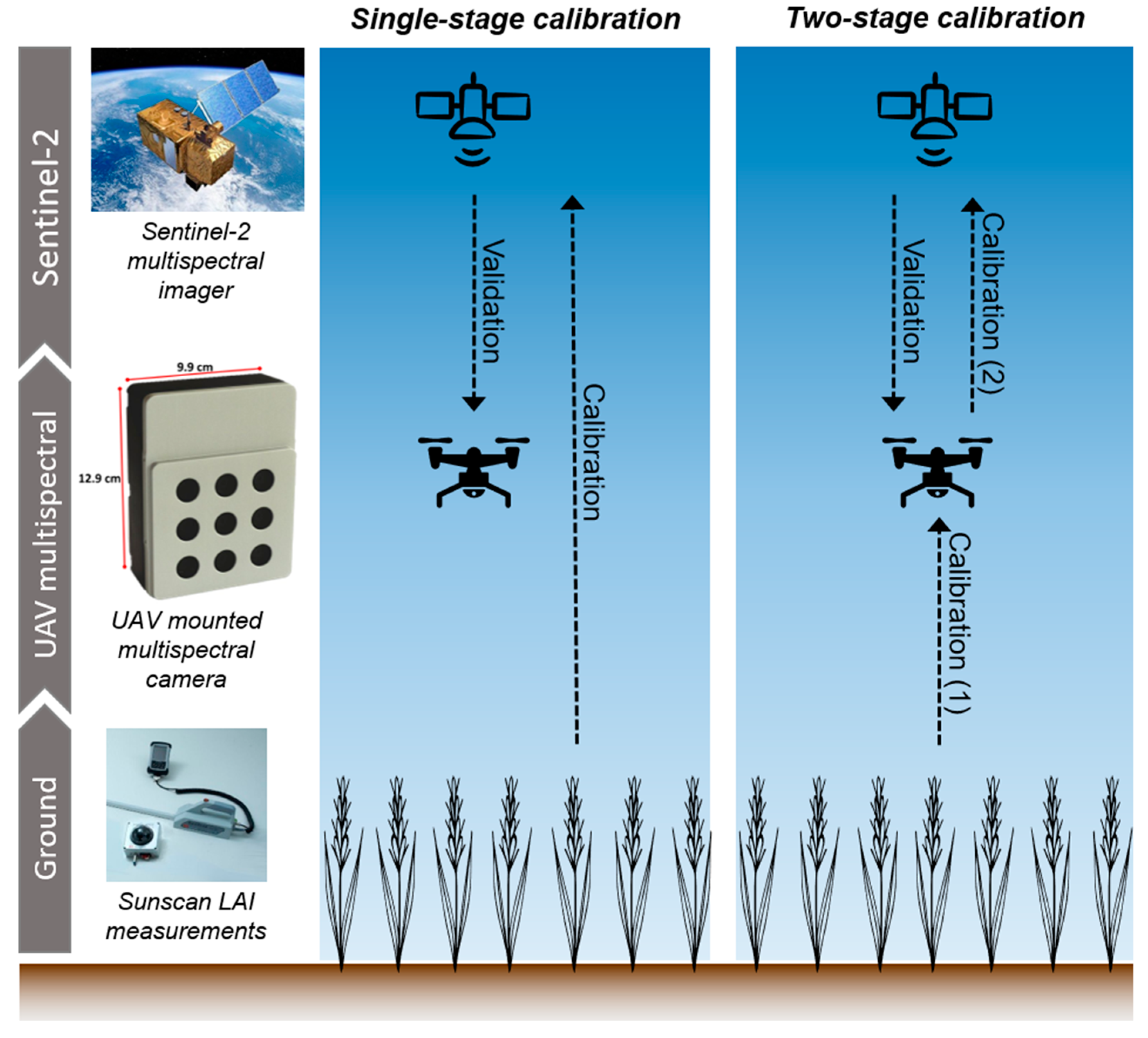
2.3.3. Sentinel-2 LAI Retrieval Approaches

For the retrieval of LAI from Sentinel-2 observations, two GPR model calibration approaches were investigated: single-stage and two-stage calibrations (Figure 3). In order to perform an independent validation of both GPR model approaches, an equal (i.e., 40/40) split was randomly applied to the 80 ground measurements in order to generate training and validation datasets. The single-stage calibration involved using the training measurements to fit the retrieval model directly to the overlapping Sentinel-2 20-m reflectance data. The two-stage calibration approach involved, first, calibrating the fine-scale UAV data with the training dataset (see Section 2.3.2). The UAV fine-scale LAI estimates are then spatially averaged to the overlapping Sentinel-2 20-m pixel grid cells. Second, the resultant spatially aggregated LAI was then used to calibrate the LAI retrieval algorithm from the Sentinel-2 spectral bands (i.e., 705 and 865 nm) used in this analysis, sampled at 20 m. The two calibration approaches were then applied to the Sentinel-2 observations covering measurement points included in the validation dataset and compared to the spatially aggregated (20 m) UAV LAI data that was also estimated using the validation dataset.

3. Results

3.1. Multiscale Chlorophyll Index Inter-Comparisons

The mean CIred-edge values derived from the UAV data were always higher than those from Sentinel-2 (mean NRMSE = 27%, Table 2). From a linear fit comparing Sentinel-2 to UAV values, for both farms, the R2 generally increased with developmental stage. The discrepancy between UAV and Sentinel-2 CIred-edge was typically larger for the earlier growth stages when compared to observations later in the season. The variance in per-farm CIred-edge values from both sensors also shows a narrowing with increasing growth stage. For the majority of growth stages, however, the variation in values derived from the UAV sensor (mean CV = 17%) was broader than that of Sentinel-2 (mean CV = 12%). The mean standard deviation of the UAV CIred-edge values (1.07) was nearly double that of the Sentinel-2 data (0.64). The difference in variance can also be seen from a probability distribution function of values from the two sensors for Farm 1 (Figure 4).

3.2. Linking UAV LAI Retrieval Accuracies to Spatial Scale

There was evidence of substantial LAI heterogeneity from comparing UAV retrievals of LAI at the scales of in-situ data (2 m). The impact of spatial scale on LAI retrievals was investigated by comparing the UAV-estimated LAI at 2-m and at 20-m spatial resolutions to in-situ measurements recorded on the ground (Figure 5). From a linear fit, the correlation with ground measurements of the LAI retrieval model calibrated with the 20-m resolution data was poor (R2 = 0.56) when compared to that of calibration with the 2-m spectral data (R2 = 0.80). The overall error between the measured and retrieved LAI was more similar for the two spatial resolutions; the NRMSEs were 11% and 13% for the 2-m and 20-m calibrations, respectively. However, bias was clearly greater when using the 20-m resolution data (particularly for LAI measurements > 3 m2 m−2) with a regression slope of 0.57, compared to 0.80 for the 2-m calibration.

3.3. Sentinel-2 LAI Retrieval Calibration Approaches

The two-stage LAI calibration approach for Sentinel-2 had a much better agreement with the validation dataset (R2 = 0.88) than the single-stage calibration (R2 = 0.29) (Figure 6). The two-stage approach could, thus, explain ~3 times as much of the variation among 20-m pixels. The error of the single-stage calibrated model (NRMSE = 17%) was more than twice that of the two-stage calibration (NRMSE = 8%). The single-stage calibration also had a large negative bias (regression slope = 0.35) when compared to the two-stage model (0.81). The single-stage calibration, thus, has major problems in identifying changes in LAI, and picking out high and low values accurately.
The observed–estimated LAI bias values in the distribution for the single-stage calibration were broader and slightly positively skewed when compared to that of the two-stage calibration (Figure 7) when using the same independent calibration/validation datasets. The two-stage calibration bias had a narrower and more symmetrical distribution. The single-stage calibration has a mean LAI error of 1.0, compared to 0.45 for the two-stage process. Furthermore, the single-stage approach produces very poorly constrained estimates in some cases, shown by the long tails of the error distribution.
The Sentinel-2 two-stage calibration was capable of resolving the within-field spatial variability in LAI, whereas the single-stage calibration only captured less than half of this variability. We compared LAI maps of sample fields derived from the different calibration approaches to that from the fine-scale UAV LAI estimates (Figure 8). The variability captured by the two-stage approach was visually comparable to the fine-scale UAV LAI estimates. In particular, the two-stage approach better resolves areas of high and low LAI. The single-stage calibration, on the other hand, appeared to underestimate LAI at higher values.
The bias and distribution of LAI estimates derived from the two calibration approaches for the field samples, in comparison with the UAV LAI data, can also be seen in the distribution plots (Figure 8). The shape of the two-stage LAI distribution matches the UAV estimates much closer when compared to that of the single-stage calibration. The single-stage calibration LAI estimates also had a much narrower distribution, which generally peaked at LAI values less than the two-stage calibration estimates, indicating a consistent and strong bias.

4. Discussion

Through a series of experiments using UAV data linked to ground measurements, we have analysed and tested approaches for minimizing spatial scaling biases and uncertainties when monitoring wheat using Sentinel-2 20-m resolution data. We quantified variation in the spectral reflectance of fields at scales below the resolution of a Sentinel-2 and found that heterogeneity within crops is an important consideration for calibrating satellite sensors. We then showed that UAV data could provide a robust bridge from in-situ data resolution to satellite pixel scale. We developed a robust calibration approach to take account of and correct for heterogeneity, and to effectively quantify retrieval error for LAI. This approach should be valid across other vegetation types for producing higher-quality biophysical retrievals.

4.1. How Do UAV and Sentinel-2 Chlorophyll Index Maps Compare across Multiple Growth Stages?

When comparing between the CIred-edge values derived from the Sentinel-2 and UAV imagery, we found that the correlation between the values from the two platforms generally increased as crop growth stage advanced. During early phenological periods, it is likely that the influence of bare soil on the reflectance spectra would have been greater, with the wheat canopy being highly heterogeneous across the field. In particular, the earlier growth stages noted for both farms (i.e., growth stages 31 and 39) correspond to the start of significant periods of canopy development, including stem elongation and the development of yield-forming leaves [11]. During this stage, when both crop ground cover and fractional light interception increase linearly with LAI [55], farmers target their main applications of nitrogen fertiliser. When compared to the relatively coarse-scale (20 m) Sentinel-2 observations, the 5-cm spatial resolution of the UAV dataset was sufficient to resolve these small discontinuities in the canopy. The distribution of values across the field was also much narrower for Sentinel-2 when compared to that of the UAV, further suggesting that these variations in canopy cover were not detected by the satellite sensor.
By later growth stages (i.e., growth stages 51 to 77), the leaf canopy is closed with the crop entering ear emergence, flowering and grain-filling phases. Correspondingly, at these growth stages, the spectral reflectance and spatial variability of the canopy across the field is generally more homogenous. Increased uniformity in the wheat canopy was also evident in the statistics where the variance and distribution of CIred-edge values estimated from the Sentinel-2 observations were comparable to those of the UAV. Studies in Fawcett et al. [56] also demonstrated a similarly high agreement between UAV and Sentinel-2 CIred-edge values during the later growth stages for maize crops.

4.2. Canopy Heterogeneity and Impact of Scale on LAI Retrieval Accuracies

Our high-resolution data confirmed that LAI was highly heterogeneous at scales below the satellite resolution (Table 2, Figure 5). The linear fit between the UAV and ground LAI was significantly better when sampled at two metres when compared to that at 20 m. The performance of GPR LAI retrieval model when calibrated with the 2-m resolution data (R2 = 0.8 and NRMSE = 11%) is also comparable to other studies with this sensor on wheat trials plots [26], where Revill et al. reported an R2 of 0.84 and NRMSE of 9%. These results together suggest that a resolution of 2 m is required to capture the variability in LAI measurements within the fields sampled. At coarser resolutions, the UAV retrieval of LAI became more biased. When investigating the retrieval of winter wheat LAI from EO data, Reichenau et al. [41] showed that even averaging data at a spatial resolution of 5 m can significantly reduce the variability in LAI when compared to ground measurements.

4.3. UAV Observations Reduced Uncertainty and Biases in Sentinel-2 LAI Retrievals

The two-stage calibration process for Sentinel-2 LAI estimates, which incorporates the upscaled ground measurements via UAV, demonstrated a clear improvement over a single-stage process without UAV data. In the two-stage process, the error was reduced by >50% in the accuracy of LAI retrievals when validated using independent ground data. As a key variable for quantifying vegetation canopy structure, accurate and consistent LAI estimates can be used directly to determine crop phenology and status (e.g., [12,57]). Past research has also demonstrated the value of LAI data for updating state variables in process-based crop models in order to improve the spatial and temporal simulation of crop dynamics, including yield and net carbon land–atmosphere exchanges (e.g., [14,15,16,17,18]).
The enhancement in LAI retrieval achieved with the two-stage GPR model calibration approach can be attributed to both an increase in the spectral purity and to the volume of samples used to train the GPR LAI retrieval models. With regards to the spectral sample purity, when training the model directly based on ground measurements (i.e., the single-stage calibration), due to accessibility with equipment and efforts to minimise crop damage, LAI measurement points would typically be constrained to the vicinity of the field tramlines (i.e., access tracks), which would bias the training dataset. Indeed, a negative bias in LAI was clear with the single-stage calibration results (Figure 6 and Figure 7). With the two-stage approach, however, the fine-scale UAV observations can resolve the spectral reflectance around and beyond the measurement points more precisely. UAV sampling reduced the influence of tramlines, by sampling the broader field and avoiding access problems for field sampling. These more representative spectral samples can be used to estimate LAI across the spatial extents of the UAV images, including areas that would not otherwise be ground-sampled, and then aggregated to match the resolution of the co-registered Sentinel-2 pixel grid.
In comparison to alternative approaches for retrieving crop variables from EO spectral reflectance, the performance of machine learning methods, including GPR, can be more sensitive to the number of ground measurements used in the training dataset [28,29]. Furthermore, unless prior knowledge of the field is available, for example through the identification of management zones [58,59,60], the within-field scale variability in in-situ LAI is typically insufficiently sampled. Our two-stage approach addresses these limitations in machine learning LAI retrieval techniques by producing accurate and high-resolution maps of the upscaling ground measurements. These upscaled measurements, which cover multiple overlapping Sentinel-2 pixels, can then be sampled and used to produce a larger training dataset when calibrating the Sentinel-2 retrieval algorithm. For instance, the number of Sentinel-2 pixels that overlapped UAV imagery on Farm 1 and 2 were 80 and 161, respectively, each of which could be used to train the LAI retrieval model.

4.4. Research Implications and Limitations

Calibrating Sentinel-2 data using fine-scale UAV estimates can produce LAI datasets that are less biased and better capture the within-field variability when compared to ground measurements. In an operational context, our two-stage UAV calibration approach could be applied, for instance, at some sample within-field areas to capture the variability in crop growth. This calibration could then be applied to larger extents of the Sentinel-2 dataset in order to generate improved estimates of wheat LAI at the farm and landscape scales.
In our study, for the first time, we have deployed a UAV sensor with Sentinel-2 matching band-pass filters. Past studies comparing UAV to satellite-scale observations (e.g., [38,56]) have used UAV instruments with different spectral bands to those of the satellite sensor. For instance, research in Dash et al. [61], which involved comparing NDVI derived from a UAV to that from the RipidEye satellite sensor, attributed the disparities in NDVI to differences in sensor spectral properties. In our research, by matching spectral observations, we reduce errors due to band-positioning off-sets. This UAV instrument, linked to the GPR modelling, provided a unique opportunity to scale up the ground measurements, whilst tracking the uncertainty of hand-held instruments, to the spatial extents of UAV flights that could then be compared to the Sentinel-2 data. We recommend future studies take advantage of such band-matching approaches.
Our study is limited to the use of spatially and temporally concurrent data (i.e., ground, UAV and Sentinel-2 acquisitions) for only one wheat growing season across two farm sites. Calibration and validation across additional growing seasons and sites would be of value to further test the performance of our two-stage calibration approach. While the calibration is specific, we would not expect our approach to be limited to wheat. We anticipate a comparably strong performance of the two-stage calibration when applied to other arable crops, and even to other vegetation types. Research in Pla et al. [38], for instance, demonstrated the calibration of Sentinel-2 NDVI using UAV data for quantifying damages to rice crops across large spatial extents. Given the typical scale mismatches between ground measurements and Sentinel-2 data, we would also expect that the two-stage calibration would be equally as valid for improving the retrieval of additional crop variables that covary with LAI, including fAPAR and canopy chlorophyll content [7,62,63]. In particular, our approach overcomes widespread calibration challenges related to resolving the spatial heterogeneity of vegetation, which are even more pressing in unmanaged/natural ecosystems. We would, therefore, recommend that the two-stage calibration, involving the use of fine-scale UAV observations, should be adopted as a standard when using Earth observations for vegetation upscaling activities.

5. Conclusions

Even within managed crop systems, we show there is considerable and important within-field variation in LAI at scales finer than the resolution of current satellite imagers. We show that UAV multispectral observations at the cm scale, acquired from a sensor designed to match Sentinel-2 spectral bands, improve interpretation of the satellite signal. Furthermore, the fine-scale resolution of the UAV sensor provides a tool for accurately upscaling LAI ground measurements, which were collected in coordination with the UAV flights, to satellite resolution. The within-field variance in spectral data resolved from the UAV observations was linked to wheat growth stage. Consequently, the Sentinel-2 and UAV platform data were more comparable at the later growth stages, when the vegetation canopy appeared more homogeneous due to a reduced influence of bare soil. Calibrating models used to retrieve LAI from Sentinel-2 observations directly from ground measurements performed poorly and were unable to explain the variance in LAI throughout the growing season. On the other hand, our novel two-stage model calibration, involving the use of upscaled UAV LAI estimates, demonstrated a clear improvement in the accuracy of LAI retrievals from Sentinel-2 data, reducing bias strongly. It would be anticipated that our approach would also improve the retrieval of additional biophysical variables for other arable crop types and a broader range of vegetation cover types. Repeating our analysis at additional field sites would be necessary in order to test the robustness of the two-stage calibration. Nonetheless, our study has highlighted the value of UAV observations for effectively providing a link between point measurements on the ground and 20-m resolution multispectral observations made from the Sentinel-2 satellite.

Author Contributions

Conceptualization, A.R., A.M. and M.W.; methodology, A.R., A.F. and M.W.; software, A.R.; validation, A.R. and M.W.; formal analysis, A.R. and M.W.; investigation, A.R.; resources, A.M. and S.H.; data curation, A.R. and A.F.; writing—original draft preparation, A.R. and M.W.; writing—review and editing, A.R., A.F., A.M., S.H., R.R. and M.W.; visualization, A.R.; funding acquisition, A.M. and M.W. All authors have read and agreed to the published version of the manuscript.

Funding

This research was funded by the joint Biotechnology and Biological Sciences Research Council (BBSRC) and National Environment Research Council (NERC) Sustainable Agricultural Research and Innovation Club (SARIC) initiative (grant numbers: BB/P004628/1 and BB/P004458/1) and NCEO.

Acknowledgments

We would like to thank the farmers on Farms 1 and 2 for consenting to the field survey campaigns carried out across their properties. Technical advice was provided by Tom Wade from the University of Edinburgh’s Airborne GeoSciences Facility. We are also grateful for the support received from the NERC National Centre for Earth Observation (NCEO) Field Spectroscopy Facility.

Conflicts of Interest

The authors declare no conflict of interest.

References

  1. Tilman, D.; Balzer, C.; Hill, J.; Befort, B.L. Global food demand and the sustainable intensification of agriculture. Proc. Natl. Acad. Sci. USA 2011, 108, 20260–20264. [Google Scholar] [CrossRef] [PubMed] [Green Version]
  2. Clark, M.; Tilman, D. Comparative analysis of environmental impacts of agricultural production systems, agricultural input efficiency, and food choice. Environ. Res. Lett. 2017, 12, 64016. [Google Scholar] [CrossRef]
  3. Gebbers, R.; Adamchuk, V.I. Precision Agriculture and Food Security. Science 2010, 327, 828. [Google Scholar] [CrossRef] [PubMed]
  4. Jat, P.; Serre, M.L. Bayesian Maximum Entropy space/time estimation of surface water chloride in Maryland using river distances. Environ. Pollut. 2016, 219, 1148–1155. [Google Scholar] [CrossRef] [Green Version]
  5. Mulla, D.J. Twenty five years of remote sensing in precision agriculture: Key advances and remaining knowledge gaps. Biosyst. Eng. 2013, 114, 358–371. [Google Scholar] [CrossRef]
  6. Chen, J.M.; Black, T.A. Defining leaf area index for non-flat leaves. Plant. Cell Environ. 1992, 15, 421–429. [Google Scholar] [CrossRef]
  7. Clevers, J.; Kooistra, L.; van den Brande, M. Using Sentinel-2 Data for Retrieving LAI and Leaf and Canopy Chlorophyll Content of a Potato Crop. Remote Sens. 2017, 9, 405. [Google Scholar] [CrossRef] [Green Version]
  8. Zhu, W.; Sun, Z.; Huang, Y.; Lai, J.; Li, J.; Zhang, J.; Yang, B.; Li, B.; Li, S.; Zhu, K.; et al. Improving Field-Scale Wheat LAI Retrieval Based on UAV Remote-Sensing Observations and Optimized VI-LUTs. Remote Sens. 2019, 11, 2456. [Google Scholar] [CrossRef] [Green Version]
  9. Zheng, G.; Moskal, L.M. Retrieving Leaf Area Index (LAI) Using Remote Sensing: Theories, Methods and Sensors. Sensors. 2009, 9, 2719–2745. [Google Scholar] [CrossRef] [Green Version]
  10. Aboelghar, M.; Arafat, S.; Saleh, A.; Naeem, S.; Shirbeny, M.; Belal, A. Retrieving leaf area index from SPOT4 satellite data. Egypt. J. Remote Sens. Sp. Sci. 2010, 13, 121–127. [Google Scholar] [CrossRef] [Green Version]
  11. Sylvester-Bradley, R.; Berry, P.; Blake, J.; Kindred, D.; Spink, J.; Bingham, I.; McVittie, J.; Foulkes, J. The Wheat Growth Guide. Available online: http://www.adlib.ac.uk/resources/000/265/686/WGG_2008.pdf (accessed on 5 May 2020).
  12. Liu, X.; Cao, Q.; Yuan, Z.; Liu, X.; Wang, X.; Tian, Y.; Cao, W.; Zhu, Y. Leaf area index based nitrogen diagnosis in irrigated lowland rice. J. Integr. Agric. 2018, 17, 111–121. [Google Scholar] [CrossRef] [Green Version]
  13. Boote, K.J.; Jones, J.W.; White, J.W.; Asseng, S.; Lizaso, J.I. Putting mechanisms into crop production models. Plant. Cell Environ. 2013, 36, 1658–1672. [Google Scholar] [CrossRef] [PubMed]
  14. Nearing, G.S.; Crow, W.T.; Thorp, K.R.; Moran, M.S.; Reichle, R.H.; Gupta, H.V. Assimilating remote sensing observations of leaf area index and soil moisture for wheat yield estimates: An observing system simulation experiment. Water Resour. Res. 2012, 48. [Google Scholar] [CrossRef] [Green Version]
  15. Revill, A.; Sus, O.; Barrett, B.; Williams, M. Carbon cycling of European croplands: A framework for the assimilation of optical and microwave Earth observation data. Remote Sens. Environ. 2013, 137. [Google Scholar] [CrossRef] [Green Version]
  16. Huang, J.; Sedano, F.; Huang, Y.; Ma, H.; Li, X.; Liang, S.; Tian, L.; Zhang, X.; Fan, J.; Wu, W. Assimilating a synthetic Kalman filter leaf area index series into the WOFOST model to improve regional winter wheat yield estimation. Agric. For. Meteorol. 2016, 216, 188–202. [Google Scholar] [CrossRef]
  17. Jin, H.; Li, A.; Wang, J.; Bo, Y. Improvement of spatially and temporally continuous crop leaf area index by integration of CERES-Maize model and MODIS data. Eur. J. Agron. 2016, 78, 1–12. [Google Scholar] [CrossRef]
  18. Li, H.; Chen, Z.; Liu, G.; Jiang, Z.; Huang, C. Improving Winter Wheat Yield Estimation from the CERES-Wheat Model to Assimilate Leaf Area Index with Different Assimilation Methods and Spatio-Temporal Scales. Remote Sens. 2017, 9, 190. [Google Scholar] [CrossRef] [Green Version]
  19. Huang, J.; Gómez-Dans, J.L.; Huang, H.; Ma, H.; Wu, Q.; Lewis, P.E.; Liang, S.; Chen, Z.; Xue, J.-H.; Wu, Y.; et al. Assimilation of remote sensing into crop growth models: Current status and perspectives. Agric. For. Meteorol. 2019, 276–277, 107609. [Google Scholar] [CrossRef]
  20. Cammarano, D.; Fitzgerald, G.; Casa, R.; Basso, B. Assessing the Robustness of Vegetation Indices to Estimate Wheat N in Mediterranean Environments. Remote Sens. 2014, 6, 2827. [Google Scholar] [CrossRef] [Green Version]
  21. Verrelst, J.; Schaepman, M.E.; Malenovský, Z.; Clevers, J.G.P.W. Effects of woody elements on simulated canopy reflectance: Implications for forest chlorophyll content retrieval. Remote Sens. Environ. 2010, 114, 647–656. [Google Scholar] [CrossRef] [Green Version]
  22. Sehgal, V.K.; Chakraborty, D.; Sahoo, R.N. Inversion of radiative transfer model for retrieval of wheat biophysical parameters from broadband reflectance measurements. Inf. Process. Agric. 2016, 3, 107–118. [Google Scholar] [CrossRef] [Green Version]
  23. Cai, Y.; Guan, K.; Lobell, D.; Potgieter, A.B.; Wang, S.; Peng, J.; Xu, T.; Asseng, S.; Zhang, Y.; You, L.; et al. Integrating satellite and climate data to predict wheat yield in Australia using machine learning approaches. Agric. For. Meteorol. 2019, 274, 144–159. [Google Scholar] [CrossRef]
  24. Hunt, M.L.; Blackburn, G.A.; Carrasco, L.; Redhead, J.W.; Rowland, C.S. High resolution wheat yield mapping using Sentinel-2. Remote Sens. Environ. 2019, 233, 111410. [Google Scholar] [CrossRef]
  25. Kayad, A.; Sozzi, M.; Gatto, S.; Marinello, F.; Pirotti, F. Monitoring Within-Field Variability of Corn Yield using Sentinel-2 and Machine Learning Techniques. Remote Sens. 2019, 11, 2873. [Google Scholar] [CrossRef] [Green Version]
  26. Revill, A.; Florence, A.; MacArthur, A.; Hoad, S.P.; Rees, R.M.; Williams, M. The value of Sentinel-2 spectral bands for the assessment of winter wheat growth and development. Remote Sens. 2019, 11. [Google Scholar] [CrossRef] [Green Version]
  27. Han, J.; Zhang, Z.; Cao, J.; Luo, Y.; Zhang, L.; Li, Z.; Zhang, J. Prediction of Winter Wheat Yield Based on Multi-Source Data and Machine Learning in China. Remote Sens. 2020, 12, 236. [Google Scholar] [CrossRef] [Green Version]
  28. Pasolli, E.; Melgani, F.; Alajlan, N.; Bazi, Y. Active Learning Methods for Biophysical Parameter Estimation. IEEE Trans. Geosci. Remote Sens. 2012, 50, 4071–4084. [Google Scholar] [CrossRef]
  29. Gewali, U.B.; Monteiro, S.T.; Saber, E. Gaussian Processes for Vegetation Parameter Estimation from Hyperspectral Data with Limited Ground Truth. Remote Sens. 2019, 11, 1614. [Google Scholar] [CrossRef] [Green Version]
  30. Liang, S.; Li, X.; Wang, J. (Eds.) Chapter 1—A Systematic View of Remote Sensing. In Advanced Remote Sensing; Academic Press: Boston, MA, USA, 2012; pp. 1–31. ISBN 978-0-12-385954-9. [Google Scholar]
  31. Delloye, C.; Weiss, M.; Defourny, P. Retrieval of the canopy chlorophyll content from Sentinel-2 spectral bands to estimate nitrogen uptake in intensive winter wheat cropping systems. Remote Sens. Environ. 2018, 216, 245–261. [Google Scholar] [CrossRef]
  32. Delegido, J.; Verrelst, J.; Alonso, L.; Moreno, J. Evaluation of Sentinel-2 red-edge bands for empirical estimation of green LAI and chlorophyll content. Sensors 2011, 11, 7063–7081. [Google Scholar] [CrossRef] [Green Version]
  33. Clevers, J.G.P.W.; Gitelson, A.A. Remote estimation of crop and grass chlorophyll and nitrogen content using red-edge bands on Sentinel-2 and -3. Int. J. Appl. Earth Obs. Geoinf. 2013, 23, 344–351. [Google Scholar] [CrossRef]
  34. Peng, Y.; Nguy-Robertson, A.; Arkebauer, T.; Gitelson, A.A. Assessment of Canopy Chlorophyll Content Retrieval in Maize and Soybean: Implications of Hysteresis on the Development of Generic Algorithms. Remote Sens. 2017, 9, 226. [Google Scholar] [CrossRef] [Green Version]
  35. Delegido, J.; Verrelst, J.; Rivera, J.P.; Ruiz-Verdú, A.; Moreno, J. Brown and green LAI mapping through spectral indices. Int. J. Appl. Earth Obs. Geoinf. 2015, 35, 350–358. [Google Scholar] [CrossRef]
  36. Xie, Q.; Dash, J.; Huete, A.; Jiang, A.; Yin, G.; Ding, Y.; Peng, D.; Hall, C.C.; Brown, L.; Shi, Y.; et al. Retrieval of crop biophysical parameters from Sentinel-2 remote sensing imagery. Int. J. Appl. Earth Obs. Geoinf. 2019, 80, 187–195. [Google Scholar] [CrossRef]
  37. Pasqualotto, N.; Delegido, J.; Van Wittenberghe, S.; Rinaldi, M.; Moreno, J. Multi-Crop Green LAI Estimation with a New Simple Sentinel-2 LAI Index (SeLI). Sensors 2019, 19, 904. [Google Scholar] [CrossRef] [PubMed] [Green Version]
  38. Pla, M.; Bota, G.; Duane, A.; Balagué, J.; Curcó, A.; Gutiérrez, R.; Brotons, L. Calibrating Sentinel-2 Imagery with Multispectral UAV Derived Information to Quantify Damages in Mediterranean Rice Crops Caused by Western Swamphen (Porphyrio porphyrio). Drones 2019, 3, 45. [Google Scholar] [CrossRef] [Green Version]
  39. Matese, A.; Toscano, P.; Di Gennaro, S.F.; Genesio, L.; Vaccari, F.P.; Primicerio, J.; Belli, C.; Zaldei, A.; Bianconi, R.; Gioli, B. Intercomparison of UAV, Aircraft and Satellite Remote Sensing Platforms for Precision Viticulture. Remote Sens. 2015, 7, 2971–2990. [Google Scholar] [CrossRef] [Green Version]
  40. Gitelson, A.A.; Gritz, Y.; Merzlyak, M.N. Relationships between leaf chlorophyll content and spectral reflectance and algorithms for non-destructive chlorophyll assessment in higher plant leaves. J. Plant Physiol. 2003, 160, 271–282. [Google Scholar] [CrossRef]
  41. Reichenau, T.G.; Korres, W.; Montzka, C.; Fiener, P.; Wilken, F.; Stadler, A.; Waldhoff, G.; Schneider, K. Spatial Heterogeneity of Leaf Area Index (LAI) and Its Temporal Course on Arable Land: Combining Field Measurements, Remote Sensing and Simulation in a Comprehensive Data Analysis Approach (CDAA). PLoS ONE 2016, 11, e0158451. [Google Scholar] [CrossRef] [Green Version]
  42. Fraser, R.H.; Van der Sluijs, J.; Hall, R.J. Calibrating Satellite-Based Indices of Burn Severity from UAV-Derived Metrics of a Burned Boreal Forest in NWT, Canada. Remote Sens. 2017, 9, 279. [Google Scholar] [CrossRef] [Green Version]
  43. Padró, J.-C.; Muñoz, F.-J.; Ávila, L.Á.; Pesquer, L.; Pons, X. Radiometric Correction of Landsat-8 and Sentinel-2A Scenes Using Drone Imagery in Synergy with Field Spectroradiometry. Remote Sens. 2018, 10, 1687. [Google Scholar] [CrossRef] [Green Version]
  44. Zadoks, J.C.; Chang, T.T.; Konzak, C.F. A decimal code for the growth stages of cereals. Weed Res. 1974, 14, 415–421. [Google Scholar] [CrossRef]
  45. Nocerino, E.; Dubbini, M.; Menna, F.; Remondino, F.; Gattelli, M.; Covi, D. Geometric Calibration and Radiometric Correction of the MAIA Multispectral Camera. ISPRS 2017, XLII-3/W3, 149–156. [Google Scholar] [CrossRef] [Green Version]
  46. Vreys, K.; VITO. Technical Assistance to fieldwork in the Harth forest during SEN2Exp; Flemish Institute for Technological Research: Boeretang, Belgium, 2014. [Google Scholar]
  47. MacLellan, C. NERC Field Spectroscopy Facility - Guidlines for Post Processing ASD FieldSpec Pro and FieldSpec 3 Spectral Data Files using the FSF MS Excel Template. 2009, 18. Available online: https://fsf.nerc.ac.uk/resources/post-processing/post_processing_v3/post%20processing%20v3%20pdf/Guidelines%20for%20ASD%20FieldSpec%20Templates_v03.pdf (accessed on 5 May 2020).
  48. European Space Agency. Copernicus Open Access Hub. Available online: scihub.copernicus.eu (accessed on 10 August 2019).
  49. Vuolo, F.; Żółtak, M.; Pipitone, C.; Zappa, L.; Wenng, H.; Immitzer, M.; Weiss, M.; Baret, F.; Atzberger, C. Data Service Platform for Sentinel-2 Surface Reflectance and Value-Added Products: System Use and Examples. Remote Sens. 2016, 8, 938. [Google Scholar] [CrossRef] [Green Version]
  50. Rasmussen, C.E.; Williams, C.K.I. Gaussian Processes for Machine Learning 2006. Available online: http://www.gaussianprocess.org/gpml/chapters/RW.pdf (accessed on 5 May 2020).
  51. Camps-Vails, G.; Gómez-Chova, L.; Muñoz-Mari, J.; Vila-Frances, J.; Amoros, J.; del Valle-Tascon, S.; Calpe-Maravilla, J. Biophysical parameter estimation with adaptive Gaussian Processes. IEEE Int. Geosci. Remote Sens. Symp. 2009, 4, IV-69–IV-72. [Google Scholar]
  52. Verrelst, J.; Rivera, J.P.; Gitelson, A.; Delegido, J.; Moreno, J.; Camps-Valls, G. Spectral band selection for vegetation properties retrieval using Gaussian processes regression. Int. J. Appl. Earth Obs. Geoinf. 2016, 52, 554–567. [Google Scholar] [CrossRef]
  53. Rivera, J.P.; Verrelst, J.; Muñoz-Marí, J.; Moreno, J.; Camps-Valls, G. Toward a Semiautomatic Machine Learning Retrieval of Biophysical Parameters. IEEE J. Sel. Top. Appl. Earth Obs. Remote Sens. 2014, 7, 1249–1259. [Google Scholar]
  54. Verrelst, J.; Muñoz, J.; Alonso, L.; Delegido, J.; Rivera, J.P.; Camps-Valls, G.; Moreno, J. Machine learning regression algorithms for biophysical parameter retrieval: Opportunities for Sentinel-2 and -3. Remote Sens. Environ. 2012, 118, 127–139. [Google Scholar] [CrossRef]
  55. Ramirez-Garcia, J.; Almendros, P.; Quemada, M. Ground cover and leaf area index relationship in a grass, legume and crucifer crop. Plant Soil Environ. 2012, 58, 385–390. [Google Scholar] [CrossRef] [Green Version]
  56. Fawcett, D.; Panigada, C.; Tagliabue, G.; Boschetti, M.; Celesti, M.; Evdokimov, A.; Biriukova, K.; Colombo, R.; Miglietta, F.; Rascher, U.; et al. Multi-Scale Evaluation of Drone-Based Multispectral Surface Reflectance and Vegetation Indices in Operational Conditions. Remote Sens. 2020, 12. [Google Scholar] [CrossRef] [Green Version]
  57. Li, Z.; Jin, X.; Yang, G.; Drummond, J.; Yang, H.; Clark, B.; Li, Z.; Zhao, C. Remote Sensing of Leaf and Canopy Nitrogen Status in Winter Wheat (Triticum aestivum L.) Based on N-PROSAIL Model. Remote Sens. 2018, 10, 1463. [Google Scholar] [CrossRef] [Green Version]
  58. Peralta, N.R.; Costa, J.L.; Balzarini, M.; Castro Franco, M.; Córdoba, M.; Bullock, D. Delineation of management zones to improve nitrogen management of wheat. Comput. Electron. Agric. 2015, 110, 103–113. [Google Scholar] [CrossRef]
  59. Buttafuoco, G.; Castrignanò, A.; Cucci, G.; Lacolla, G.; Lucà, F. Geostatistical modelling of within-field soil and yield variability for management zones delineation: A case study in a durum wheat field. Precis. Agric. 2017, 18, 37–58. [Google Scholar] [CrossRef]
  60. Guo, C.; Zhang, L.; Zhou, X.; Zhu, Y.; Cao, W.; Qiu, X.; Cheng, T.; Tian, Y. Integrating remote sensing information with crop model to monitor wheat growth and yield based on simulation zone partitioning. Precis. Agric. 2018, 19, 55–78. [Google Scholar] [CrossRef]
  61. Dash, P.J.; Pearse, D.G.; Watt, S.M. UAV Multispectral Imagery Can Complement Satellite Data for Monitoring Forest Health. Remote Sens. 2018, 10. [Google Scholar] [CrossRef] [Green Version]
  62. Gitelson, A.A.; Viña, A.; Ciganda, V.; Rundquist, D.C.; Arkebauer, T.J. Remote estimation of canopy chlorophyll content in crops. Geophys. Res. Lett. 2005, 32. [Google Scholar] [CrossRef] [Green Version]
  63. Zhang, F.; Zhou, G.; Nilsson, C. Remote estimation of the fraction of absorbed photosynthetically active radiation for a maize canopy in Northeast China. J. Plant Ecol. 2014, 8, 429–435. [Google Scholar] [CrossRef] [Green Version]
Figure 1. Locations of two farms (red dots) and map insets highlighting the field sites (red border) and within-field areas of interest (black cross-hatching) where field campaign data, including ground measurement and UAV surveys, were carried out.
Remotesensing 12 01843 g001
Figure 2. Sample CIred-edge image over a field on Farm 2 shown for the high-resolution (5 cm) UAV CIred-edge imagery (acquired on 23 May 2018) with an overlapping sampling grid generated from the Sentinel-2 20-m pixels.
Remotesensing 12 01843 g002
Figure 3. Overview of approaches for calibrating GPR models used for retrieving LAI from Sentinel-2 data. Including: single-stage calibration based on ground measurements and indirect calibration involving, first, upscaling ground measurement using high-resolution UAV data and, second, calibrating the Sentinel-2 retrieval model based on UAV LAI data. Validation of both approaches performed using UAV data averages per Sentinel-2 pixel.
Remotesensing 12 01843 g003
Figure 4. Scatter plot comparisons of the mean and distribution of CIred-edge values derived from coarse-scale Sentinel-2 and fine-scale UAV observations aggregated to 20 m for Farm 1. This includes slope values used to quantify bias and a dashed gray line representing the 1:1 line. Joint histograms of values from both sensors include the kernel density fit (solid black line).
Remotesensing 12 01843 g004
Figure 5. Scatter plot comparisons between LAI retrieval models calibrated with UAV multispectral data aggregated at 2 m (left) and aggregated to a 20 × 20 m square grid cell (right). Both calibration approaches are compared to LAI ground measurements acquired at 80 locations. Plot includes a liner fit line (solid green line) with 68% confidence interval (shaded green area). The dashed gray line represents the 1:1 line.
Remotesensing 12 01843 g005
Figure 6. Independent validation of Sentinel-2 LAI (S2-LAI) to UAV spatially aggregated (20 m) LAI estimates (UAV-LAI). S2-LAI include estimates from a direct single-stage LAI retrieval calibration using ground data (left) and a two-stage calibration using the spatially up-scaled (20 m) UAV LAI estimates (right). Dashed gray line represents the 1:1 line.
Remotesensing 12 01843 g006
Figure 7. Comparison of observed–modelled LAI bias probability distribution function plots for the single-stage (blue line and shading) and two-stage (green line and shading) calibration approaches.
Remotesensing 12 01843 g007
Figure 8. Example LAI maps and distributions of three fields. From the top row, fine-scale UAV LAI estimates (row 1), Sentinel-2 estimates derived from the single-stage GPR model calibration (row 2), estimates from the two-stage calibration (row 3) and plots comparing the distribution of LAI values amongst the UAV and GPR model estimates (row 4).
Remotesensing 12 01843 g008
Table 1. Dates of the UAV data acquisition and ground measurements across the within-field regions of interest at Farms 1 and 2, along with the corresponding average winter wheat growth stage (Zadoks scale) and nearest Sentinel-2 imagery date (within +/− 5 days of the Sentinel-2 overpass).
FarmUAV/Ground Observation Date (2018)Growth Stage (Description)Sentinel-2 Observation Date (+/− UAV Day)
Farm 124th May39 (Stem elongation—late)25th May (+1)
Farm 15th June51 (Ear emergence)7th June (+2)
Farm 128th June69 (Flowering completed)29th June (+1)
Farm 24th May31 (Stem elongation—early)5th May (+1)
Farm 223rd May39 (Stem elongation—late)28th May (+5)
Farm 23th July77 (Milk development)4th July (+1)
Table 2. Summary statistics for CIred-edge, derived from samples extracted from a Sentinel-2 20-m pixel grid, quantifying multi-temporal differences between coarse-scale Sentinel-2 and fine-scale resolution UAV values averaged per Sentinel-2 grid cell. Metrics, reported per farm and growth stage (GS), include number of pixels sampled, mean value, standard deviation (SD) and coefficient of variation (CV), coefficient of determination (R2) and normalised-root-mean-square error (NRMSE).
Sentinel-2 CIred-edge (20 m)UAV CIred-edge (0.05 m)Sentinel-2/UAV Inter-Comparisons
FarmGSNumber of PixelsMeanSDCV (%)Number of PixelsMeanSDCV (%)R2NRMSE (%)
Farm 139807.460.81115,491,4838.881.18130.3728
Farm 151807.070.92135,491,4839.621.10110.7545
Farm 168805.940.5195,491,4836.140.4780.6514
Farm 2311611.840.422311,051,6102.490.76310.3232
Farm 2391618.590.75911,051,6109.152.09230.5819
Farm 2781614.290.451011,051,6105.570.82150.7123
Average0.6412 1.07170.5627

