WaterNet: A Convolutional Neural Network for Chlorophyll-a Concentration Retrieval

Abstract

The retrieval of chlorophyll-a (Chl-a) concentrations relies on empirical or analytical analyses, which generally experience difficulties from the diversity of inland waters in statistical analyses and the complexity of radiative transfer equations in analytical analyses, respectively. Previous studies proposed the utilization of artificial neural networks (ANNs) to alleviate these problems. However, ANNs do not consider the problem of insufficient in situ samples during model training, and they do not fully utilize the spatial and spectral information of remote sensing images in neural networks. In this study, a two-stage training is introduced to address the problem regarding sample insufficiency. The neural network is pretrained using the samples derived from an existing Chl-a concentration model in the first stage, and the pretrained model is refined with in situ samples in the second stage. A novel convolutional neural network for Chl-a concentration retrieval called WaterNet is proposed which utilizes both spectral and spatial information of remote sensing images. In addition, an end-to-end structure that integrates feature extraction, band expansion, and Chl-a estimation into the neural network leads to an efficient and effective Chl-a concentration retrieval. In experiments, Sentinel-3 images with the same acquisition days of in situ measurements over Laguna Lake in the Philippines were used to train and evaluate WaterNet. The quantitative analyses show that the two-stage training is more likely than the one-stage training to reach the global optimum in the optimization, and WaterNet with two-stage training outperforms, in terms of estimation accuracy, related ANN-based and band-combination-based Chl-a concentration models.

1. Introduction

Eutrophication occurs when a water body becomes overly enriched with nutrients, e.g., phosphorus and nitrogen. Aquaculture managers add nutrient fertilizers to increase the density and productivity of commercial fish. However, the oversupply of nutrients might cause eutrophication, and consequently, algal blooms which refer to excessive algal growth due to the increased availability of nutrients arise that causes the degradation of water quality [1]. Several works reported that Europe and USA suffer economic losses of approximately 1 billion and 100 million USD per year, respectively, due to eutrophication [2,3]. The avoidance of eutrophication and the monitoring of Chl-a concentrations are thus important not only for the improvement of human health but also for the reduction of financial losses.

Long-term water quality monitoring and measurement is necessary and has become a growing global concern. The collection of reliable water quality data is crucial to enable administrators to understand the types and severity of water quality impairments. The conventional approach, which involves collecting and analyzing water samples in a professional laboratory, can accurately extract water quality parameters, such as chlorophyll-a (Chl-a) concentration, colored dissolved organic matter (CDOM), and total suspended sediment, at few sampling stations. However, this approach is labor intensive and time consuming when long-term monitoring and management are required.

Several researchers proposed the utilization of optical satellite images for water quality monitoring in the 1970s. Since then, numerous satellite images and methods have been proposed to link the spectral information of remote sensing images and the water quality parameters, especially Chl-a concentrations which is a measure of phytoplankton biomass and frequently used to indicate algal blooms [4]. For example, Ha et al. [5], Kown et al. [6], and Van Nguyen et al. [7] used Landsat-8 OLI sensor which provides a moderate spatial resolution, which is 30 m $\times$ 30 m for a pixel. However, in addition to that designed for land, the Landsat-8 image has only five spectral bands available for the purpose of water bodies. On the other occasion, González Vilas et al. [8], Li et al. [9], and Zhang et al. [10] utilized Medium Resolution Imaging Spectrometer (MERIS) images to assess the Chl-a concentrations estimation. MERIS images are dedicated for water and provide a more detailed variation in spectral resolution with 15 spectral bands available for assessing in-water parameters. MERIS images cover 300 m $\times$ 300 m in reality, better than the other water-dedicated images such as SeaWIFS, MODIS, and NOAA. Cristina et al. [11] and Toming et al. [12] preferred to employ Sentinel-3 image which continues the legacy of MERIS image whose operation was ended in 2012. It even has similar spatial resolution, and Sentinel-3 provides six additional spectral bands than MERIS image and has recently become the most advanced water-dedicated image [13]. The signals recorded at at-sensor radiance are partially contributed from photons scattered by gases and aerosols in atmosphere. The main challenge in using such orbital data is the removal of atmospheric effects [14]. The methods to remove atmospheric effects, called atmospheric correction, can be classified as absolute and relative correction. The absolute correction predicts and removes the scattering due to gases and aerosols in the atmosphere [15,16], and several models have been proposed for water bodies [17,18,19]. By contrast, the relative correction minimizes numerical differences among images using image processing techniques [20,21,22,23].

Once the atmospheric effect is reduced, the remote sensing reflectance ($R_{rs}$) is used in Chl-a concentration estimation. The methods to estimate the Chl-a concentration from $R_{rs}$ can be classified into empirical- and analytical-based methods. Empirical models are generally based on regression between Chl-a concentrations and $R_{rs}$ of spectral bands (e.g., single band, multiple bands, and band combination) [24,25,26]. Dall’Olmo and Gitelson [27] proposed a three-band model that employs the maximum ratio of the remote sensing reflectance of two blue (443 and 490 nm) and one green spectral band (560 nm) to determine Chl-a concentrations. On the other occasion, Al Shehhi et al. [28] utilized red spectral band (645 nm) instead of green (560 nm) in the three-band modelling. Researchers converted and simplified a three-band model into a two-band model, in which the blue spectral band at 443 nm was removed [29,30]. With respect to the appreciable information in the spectral domain, Barnes et al. [31] utilized all available bands of the MERIS sensor in band combinations to develop a Chl-a retrieval model, and several methods [7,10,32,33,34] determine important features which are sensitive to Chl-a concentration from a pool of band combination. Take Sentinel-3 satellite images and a two-band combination as an example. With 16 spectral bands of Sentinel-3, the number of combinations of the two band ratio are $C_2^{16}$, which means that 120 candidates are available for Chl-a concentration estimation. The combination can be extended to three- and even four-band combinations, and the function in the band ratio can be altered by other functions. These changes result in a large pool of feature candidates. In contrast to empirical methods, analytical methods [35,36] transform remote sensing reflectance into the inherent optical properties (IOPs) of water using the radiative transfer equation (RTE) and further link the estimated IOPs to Chl-a concentrations. However, the accuracy of Chl-a concentration retrieval might be unstable because of the difficulty of approximating the spectral shapes of IOPs [37].

Artificial neural networks (ANNs) have been utilized in geospatial fields with various applications [8,38,39,40]. ANN is called glorified regression because of the network’s nonlinear modeling feature. Ioannou et al. [37,41] used ANN instead of RTE to model IOP coefficients from simulated $R_{rs}$. The obtained IOP coefficients were then used to retrieve Chl-a concentrations. Buckton et al. [42] proposed an ANN-based empirical model that directly links $R_{rs}$ to Chl-a concentrations. A three-layer structure, consisting of input, hidden, and output layers, was adopted in these ANN-based studies, and the results reveal the capability of ANNs to retrieve Chl-a concentrations. Furthermore, Hafeez et al. [43] searched for the optimal neural structure and parameters including the number of hidden layers and neurons by using exhaustive search. The study further compared the determined optimal ANN model with models based on other machine learning methods, including random forest, cubist regression, and support vector regression, for Chl-a concentration estimation. The experimental results revealed that the optimal ANN model has better performance. However, these ANN-based models are pixel-based models, and thus, Chl-a concentrations are estimated from the variations of the remote sensing reflectance in the spectral bands of a pixel. In other words, the models do not consider local spatial information.

In addition, ANN-based models suffer from the problem of insufficient in situ samples. Training an ANN model requires a large set of labelled samples and good initial values for optimization. Training with few samples will lead to overfitting problems, and unsuitable initial values will make the convergence of the loss function to the global minimum difficult. Kown et al. [6] utilized around 90 in situ Chl-a concentration samples in the middle of the South Sea of Korea to train a three-layered ANN. Similar quantity was also acquired by El-habashi et al. [44]. Some researchers utilized a spectra simulation technique, such as Hydrolight and WASI3D, to simulate the $R_{rs}$ and Chl-a concentration samples for data enrichment, and the simulated samples were further used to train the ANN models [37,41,42]. Ioannou et al. [37] reported that a slight underestimation appeared, possibly because of the simulation.

In the present study, a Chl-a concentration estimation model based on a convolutional neural network (CNN), called WaterNet, is proposed. WaterNet is an end-to-end model that integrates feature extraction, band expansion, and Chl-a estimation into the neural network. 3D convolutional kernels are utilized in which both spectral and spatial information in images are adopted in the neural network. Therefore, the proposed WaterNet can handle artificial objects in water bodies, such as aquaculture cages and aquatic plants, and alleviate the influence of satellite instrumental errors. In addition, a two-stage training consisting of pretraining and refinement is proposed to address sample insufficiency. WaterNet is pretrained by utilizing the Chl-a concentrations derived from an existing Chl-a concentration model in the first stage. Then, the in situ samples are used to refine the pretrained model in the second stage. The proposed method provides two contributions: (1) the introduction of WaterNet, which is an end-to-end CNN-based model; and (2) the introduction of a two-stage training that can alleviate the problem of insufficient in situ samples.

2. Materials and Methods

2.1. Study Area and Datasets

The study area is Laguna Lake (Figure 1), which is the largest lake in the Philippines with an area of 900 ${\mathrm{km}}^2$. The average depth is 2.8 $\mathrm{m}$ and the shoreline length is 220 $\mathrm{km}$. The water resources of Laguna Lake are used to provide water supply, enable the transportation of people and goods between communities, and support the aquaculture industry [45]. The aquaculture structures occupy nearly 150 ${\mathrm{km}}^2$ (around 17%) of the total lake area and most are fish farms including 14 indigenous species and 19 exotic species [46]. The rapid growth of the population and urbanization in Manila is producing large amounts of wastewater and inorganic materials, which threaten the water quality of Laguna Lake.

Field data were collected on five different days in January–April 2019, covering up the dry season. Completing the collection of all samples in one campaign and one day is difficult because of the huge area of the lake. Therefore, the study area was divided into three regions: West Bay, Central and South Bays, and East Bay, and the samples in one region were collected in each campaign. The starting point and time to take samples were on a local port located in-between the West and Central Bays and at around 8 a.m. to match the satellite acquisition time. Completing a field survey in West or Central Bay requires around 5 h, excluding the installation and uninstallation of the tools on the boat. Going to the East Bay from the port requires 2–3 more hours, and the survey might not able to match the sampling and acquisition time. Therefore, no data were collected in East Bay during the period.

An along-track Chl-a data logger, Infinity-CLW ACLW2-USB produced by JFE Advantech Co., Ltd., was installed on a boat with a depth of 0.5 m to measure the Chl-a concentrations for each second, while speed of the boat was around 10 kph. The Chl-a data logger recorded around 15,000 samples in one campaign. However, several successive samples were mapped to a pixel in the satellite images because of the differences between the sampling resolution and the image spatial resolution. Moreover, outlier removal and data aggregation were performed in data preprocessing to partially remove noises from the measured Chl-a concentrations. Specifically, a sample was removed if two successive records of Chl-a concentrations showed considerable differences or if the Chl-a concentrations exceeded the interquartile range of the dataset collected in one campaign. Then, the Chl-a concentration of a water pixel was obtained by averaging the Chl-a concentrations of the samples that were geographically mapped to that pixel. A total of 257 in situ samples were collected from the field campaigns. The statistical information of the in situ samples is summarized in

Table 1. Summary of field campaigns in 2019 (fourth column: number of samples; fifth column: range of chlorophyll-a (Chl-a) concentrations).

Campaign	Date	Region	Samples #	Chl-a Conc. (μg/L)
1st	January 11	West	35	11.339 ± 0.592
2nd	March 29	Center	74	7.906 ± 0.165
3rd	April 6	West	98	8.483 ± 1.230
4th	April 26	Center	22	7.254 ± 0.323
5th	April 30	West	48	9.598 ± 0.822
Total samples			257	8.639 ± 1.538

.

Sentinel-3 was launched by the European Space Agency as a part of the Copernicus Programme. Sentinel-3 was expected to continue the legacy of the MERIS in extracting a wide range of information about optically significant constituents in water bodies. Therefore, Sentinel-3 OLCI images were selected as remote sensing images in the current work. The satellite carries seven sensors, including Ocean and Land Color Instrument (OLCI) which contains 21 spectral bands with the wavelengths ranging from visible to near-infrared. To avoid the atmospheric effect, this study adopts level-2 water full-resolution (WFR) images which contain 16 atmospherically-corrected spectral bands of 300 m spatial resolution, including Bands 1–12, 16–17, and 20–21, and two Chl-a concentration channels built by using the inverse radiative transfer model-neural network (IRTM-NN) [47] and OC4Me [48]. As for the other bands, Bands 13–15 and Bands 18–19 were dedicated for atmospheric correction and were not available in level-2 WFR. Five level-2 water full-resolution (WFR) images over the study area were utilized.

Non-water pixels, including the pixels belonging to land and clouds, did not have information about Chl-a concentrations. In addition, the remote sensing reflectance of some water pixels are outside the normal range (0–1 sr⁻¹) possibly because of the existence of cloud shadows or the low acquisition quality. In addition to WFR, the OLCI global vegetation index in land full-resolution (LFR) level-2 images was utilized in the classification. Using the WFR and LFR of Sentinel-3 level-2 images, the images were classified as water, land, cloud, cloud shadow, and low-quality water pixels. A classification based on a decision tree was adopted. The classification results for the tested Sentinel-3 images are displayed in Figure 2.

2.2. CNN-Based Chl-a Concentration Model

In this section, the data preprocessing and normalization (Section 2.2.1), WaterNet network structure (Section 2.2.2), and proposed two-stage training (Section 2.2.3) are introduced and discussed.

2.2.1. Data Preprocessing and Normalization

WaterNet adopts a 3D convolution kernel, which utilizes the spatial and spectral information of images in modeling instead of pixel-based structure and spectral information. The input to WaterNet is a volume of the size $7\times 7\times 16$. The volume covers a small patch centered at a water pixel. The selection of $7\times 7$ spatial coverage for WaterNet input is because of the padding effect that arises from convolutional processes. Each pixel in the patch contains the normalized remote sensing reflectance of the 16 spectral bands of Sentinel-3 WFR level-2 images. The output of WaterNet is the estimated normalized Chl-a concentration at the center pixel of the input patch.

During data preprocessing, the cloud- and shadow-free water pixels are extracted from the images, and patching is performed to create a local patch with a size of $7\times 7$ for each pixel. To provide a roughly estimated Chl-a concentration for each patch, we used the Chl-a concentrations at the center pixel of a patch estimated by IRTM-NN and OC4Me.

Table 2. Image patch summary with corresponding image-based Chl-a conc. estimations on each campaign.

Campaign #	# of Patches	Chl-a Conc. (μg/L) at Center Pixel
		IRTM-NN	OC4Me
1st	1008	1.348 ± 0.034	0.983 ± 0.052
2nd	4715	1.321 ± 0.022	0.993 ± 0.069
3rd	5681	1.327 ± 0.039	0.987 ± 0.104
4th	1809	1.236 ± 0.060	1.138 ± 0.156
5th	2582	1.210 ± 0.082	1.095 ± 0.176
All samples	20,565	1.299 ± 0.072	1.055 ± 0.106

summarizes the number of image patches, those with non-water pixels are excluded, mapped to the cloud- and shadow-free water samples in the campaigns, as well as the Chl-a concentration at the patch center pixel estimated by IRTM-NN and OC4Me.

After the preprocessing, a set of patches with roughly estimated Chl-a concentrations can be obtained, that is, $\left\{\left(Patc{h}_1,c_1\right),\cdots ,\left(Patc{h}_{n_p},c_{n_p}\right)\right\}$, where $n_p$ denotes the number of patches, $Patc{h}_i=\left\{r_1^i,\cdots ,r_{49}^i\right\}$ represents the remote sensing reflectance set of the 49 pixels in the ith patch, and $c_i$ denotes the Chl-a concentration of the center pixel in the ith patch calculated with IRTM-NN or OC4Me. In addition, a small set of patches with in situ Chl-a measurements from field campaigns are utilized: $\left\{\left(Patc{h}_{m\left(1\right)},i{s}_{m\left(1\right)}\right),\cdots ,\left(Patc{h}_{m\left(n_{is}\right)},i{s}_{m\left(n_{is}\right)}\right)\right\}$, where $n_{is}$ denotes the number of in situ samples, $m(.)$ is the mapping function between the indexes of the in situ samples and the samples with estimated Chl-a concentrations, and $i{s}_{m\left(j\right)}$ is the measured Chl-a concentration in jth in situ sample. The Chl-a concentrations of the patches are normalized to the range [0, 1] using the following equations for model training stabilization:

$$n\_c_i=\left(c_i-min\left(chla\right)\right)/\left(max\left(chla\right)-min\left(chla\right)\right)$$

(1)

$$n\_i{s}_{m\left(j\right)}=\left(i{s}_{m\left(j\right)}-min\left(chla\right)\right)/\left(max\left(chla\right)-min\left(chla\right)\right)$$

(2)

where $n\_c_i$ and $n\_i{s}_{m\left(j\right)}$ denote the normalized c_i and $i{s}_{m\left(j\right)}$, respectively; $max\left(chla\right)$ and $min\left(chla\right)$ represent the maximal and minimal values of the roughly estimated or in situ Chl-a concentrations, respectively. Similarly, the pixel remote sensing reflectance is rescaled to the range [0, 1] as

$$n\_r_i=\left(r_i-min\left(R\right)\right)/\left(max\left(R\right)-min\left(R\right)\right)$$

(3)

where $n\_r_i$ is the normalized remote sensing reflectance of spectral bands $r_i$, $max\left(R\right)$ and $min\left(R\right)$ represent the maximal and minimal values of the remote sensing reflectance at each wavelength, respectively, and $R\in {\mathbb{R}}^{16\times n_p}$ is the set of the remote sensing reflectance of all pixels. After the preprocessing, two normalized sample sets, namely, ${\left\{\left(n\_Patc{h}_i,n\_c_i\right)\right\}}_{i=1}^{n_p}$ and ${\left\{\left(n\_Patc{h}_{m\left(j\right)},n\_i{s}_{m\left(j\right)}\right)\right\}}_{j=1}^{n_{is}}$, can be obtained and used in the model training, where $n\_Patc{h}_i=\left\{n\_r_1^i,\cdots ,n\_r_{49}^i\right\}$ represents the set of normalized pixels in patch i.

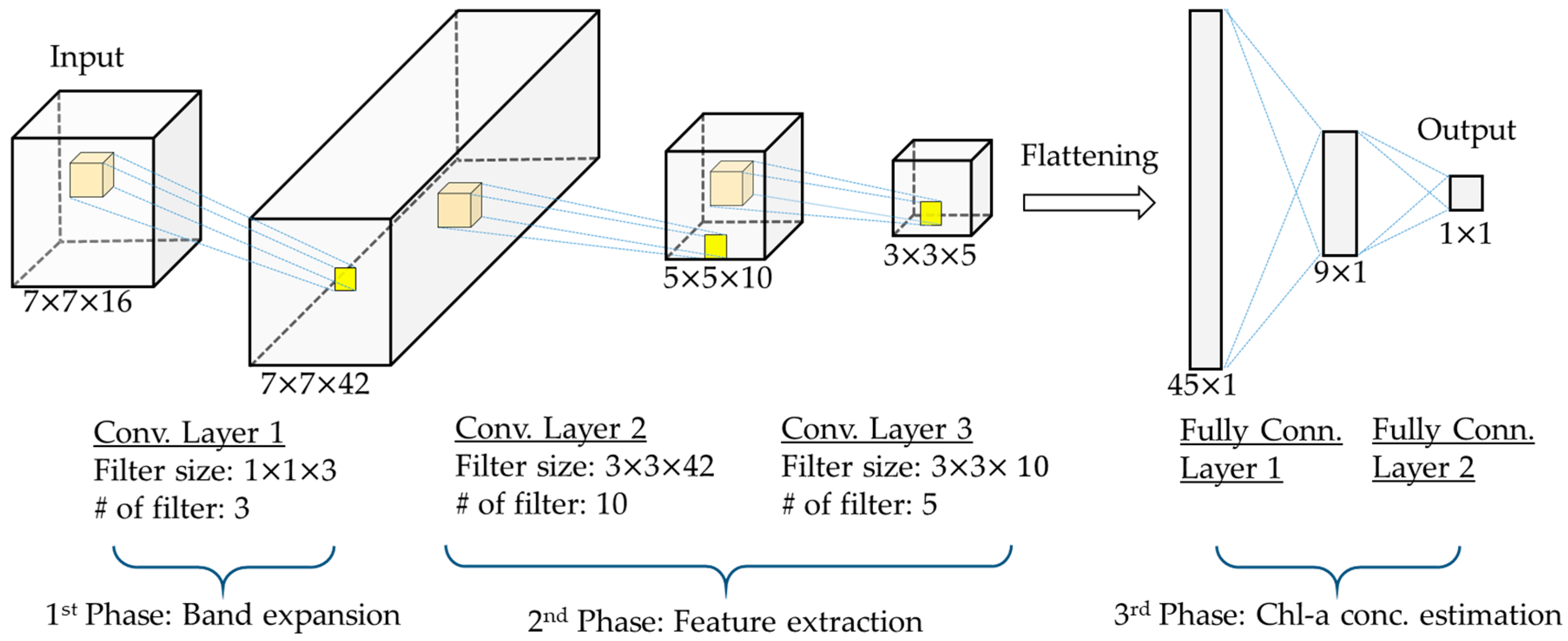
2.2.2. Network Structure of WaterNet

Figure 3 illustrates the network structure of WaterNet, which consists of three phases: band expansion, feature extraction, and Chl-a estimation. WaterNet contains one 3D convolution layer in the first phase, two 3D convolution layers in the second phase, and two fully connected layers in the third phase. The three phases are described below.

Band expansion phase. In line with the works of [5,49,50], who utilized band combinations as feature candidates in Chl-a concentration modeling, this phase aims to enrich the spectral information using band combination. The filter’s kernel size used in this phase is $1\times 1\times 3$, indicating that the convolution is performed in the spectral domain and that spectral enrichment is achieved using linear band combination. A rectified linear unit function is used as an activation function, followed by batch normalization. This phase involves three filters and 24 unknown parameters. Half of these parameters are weights and biases in the filter masks while the others include means, standard deviations, shifts, and scaling in batch normalization. Moreover, no padding is adopted during filtering, and the output of the layer is a $7\times 7\times 42$ feature volume, where $7\times 7$ is the spatial size and 42 is the spectral size.

Feature extraction phase. This phase involves two 3D convolutional layers that extract the features that are sensitive to Chl-a concentration. In the first layer, 10 filter kernels with a size of $3\times 3\times 42$ are utilized to produce 10 feature maps. The spatial size of the feature maps in the first convolutional layer is $5\times 5$ because of the absence of padding during filtering. The second convolutional layer utilizes five filter kernels with a size of $3\times 3\times 10$. The output of this layer is a $3\times 3\times 5$ feature volume. In total, this phase involves 4305 unknown parameters, including 3830 in the first convolutional layer and 475 unknowns in the second one.

Chl-a estimation phase. The Chl-a estimation phase involves reshaping a 3D volume into a 1D vector by flattening and two fully connected layers. The length of the reshaped vector is 45 because the size of the output from the second phase is $3\times 3\times 5$. The vector is fully connected to a hidden layer with nine neurons and is further fully connected to an output layer with one neuron representing the normalized Chl-a concentration at the patch center pixel. A sigmoid function is used as an activation function in the fully connected layers. A total of 424 unknown parameters are involved in this phase.

Several studies on remote sensing using ANN conducted experiments to search for the optimal neural network structure and parameters, including filter sizes, number of filters, number of layers, number of neurons, and even activation functions. This process is generally trial-and-error and time-consuming. In addition, searching for the optimal neural structure with optimal parameters is sometimes not suitable because of the limited in-situ samples and overfitting problem. Therefore, this study addresses the design of the phrases in neural structures instead of the optimal parameters.

2.2.3. Two-Stage Training

WaterNet containing 4753 unknown parameters requires a large number of in situ samples for training to reach global optimization. However, in situ sample collection is costly, and only 257 in situ samples were obtained from the field campaigns in this work. The number of in situ samples for training is much less than the number of unknowns in WaterNet. Training with insufficient samples will increase the probability of generalization errors and overfitting. In addition, setting the initial values for the unknown parameters in the optimizer is crucial, especially when the training samples are insufficient. To solve this problem, this work introduces a two-stage training consisting of pretraining and refinement. In the former, WaterNet is pretrained using the samples with Chl-a concentrations derived from an existing retrieval model (i.e., ${\left\{\left(n\_Patc{h}_i,n\_c_i\right)\right\}}_{i=1}^{n_p}$). The pretrained model is refined with the in situ samples in the latter stage (i.e., ${\left\{\left(n\_Patc{h}_{m\left(j\right)},n\_i{s}_{m\left(j\right)}\right)\right\}}_{j=1}^{n_{is}}$). The concept of the two-stage training is illustrated in Figure 4. The main idea is to obtain a suitable initial value through a pretraining process with the labeled samples obtained from an existing Chl-a model. In other words, a set of patch samples with roughly estimated Chl-a concentrations are generated by using an estimation model. The calculated loss values, however, may exhibit large deviations because the sample labels and Chl-a concentrations are not as accurate as the in situ measurements. Nevertheless, the pretraining result is closer to the real optimum compared with the initial values. The pretraining result is thus used as the new initial value in the refinement stage. Using in situ samples as training samples with the new initial values has a higher probability to reach the global optimum, compared with one-stage training, i.e., training using samples from an existing model or from in situ measurements. In this way, the requirement of large in situ sample sets can be reduced because of the two-stage training strategy.

Two candidates of Chl-a concentrations are provided in Sentinel-3 WFR products, namely, Chl-a concentrations from IRTM-NN and OC4Me. IRTM-NN is an analytical-based method that replaces RTE with an ANN with 10 spectral bands in the input layer, and OC4Me is a two-band model [51]. These two candidates are compared with the in situ Chl-a concentrations, and the one with better accuracy in terms of root mean square error (RMSE) is utilized to generate labeled samples. On the basis of the comparisons shown in

Table 3. Comparison of Chl-a concentration estimations between inverse radiative transfer model-neural network (IRTM-NN) and OC4Me.

Campaign	In Situ Samples (μg/L)		RMSE (μg/L)
	# of Samples	Chl-a Conc.	IRTM-NN	OC4Me
1st	35	11.339 ± 0.592	10.008	10.361
2nd	74	7.906 ± 0.165	6.591	6.917
3rd	98	8.483 ± 1.230	7.251	7.613
4th	22	7.254 ± 0.323	6.109	5.856
5th	48	9.598 ± 0.822	8.420	8.538
Average		8.639 ± 1.538	7.676	7.857

, the estimated Chl-a concentrations from IRTM-NN are slightly better than those from OC4Me. Therefore, IRTM-NN is selected and used to generate the labeled sample ${\left\{\left(n\_Patc{h}_i,n\_c_i\right)\right\}}_{i=1}^{n_p}$ for the pretraining.

In optimization, the Adam optimizer which utilizes adaptive learning rate and moment is employed [52], and the MSE is used as the loss function. Given the labeled samples $\left\{n\_c_1,\cdots ,n\_c_{n_p}\right\}$ and the corresponding predictions $\left\{pred{i}_1,\cdots ,pred{i}_{n_p}\right\}$ from the model, the loss function is defined as

$$L=\frac{1}{n_p}{{\displaystyle \sum }}_{i=1}^{n_p}{\left(pred{i}_i-n\_c_i\right)}^2$$

(4)

Overfitting is alleviated by adopting the commonly used dropout and $L_2$ regularization. The dropout temporally removes several neurons when computing the loss function for model convergence monitoring, whereas the $L_2$ regularization penalizes large weights by adding the Frobenius norm of parameters to the loss function (Equation (3)) during error backpropagation for weights tuning. In training, the number of epochs is set to 30, and the training process stores the parameters of the epoch with the minimal loss value. These values, along with the network structure, are used to estimate Chl-a concentrations.

2.2.4. Postprocessing of WaterNet

The output of WaterNet is the estimated normalized Chl-a concentration. Therefore, postprocessing is performed to transform the normalized Chl-a concentration back to the original range using the maximal and minimal values of the Chl-a concentrations in Equation (1). The recalling is defined as

$${\widehat{chl\_a}}_i=n\_{\widehat{chl\_a}}_i\left(max\left(chl\_a\right)-min\left(chl\_a\right)\right)+min\left(chl\_a\right)$$

(5)

where $n\_{\widehat{chl\_a}}_i$ represents the estimated normalized Chl-a concentration from WaterNet, and ${\widehat{chl\_a}}_i$ is the estimated Chl-a concentration after rescaling.

3. Experimental Results

To evaluate the performance of WaterNet, we adopted the k-fold cross-validation, in which k is set to 10 and all samples from the campaigns were uniformly partitioned into 10 folds.

Table 4. Chl-a concentration distribution in each fold.

Fold ID	Chl-a Conc. (μg/L)
	Mean	Std.	Max.	Min.
1	9.134	1.617	12.463	6.753
2	9.043	1.532	12.150	6.840
3	8.936	1.389	11.586	6.932
4	8.980	1.399	11.692	7.079
5	8.980	1.354	11.552	7.139
6	8.956	1.348	11.488	7.099
7	8.968	1.362	11.847	7.099
8	8.928	1.446	11.916	6.738
9	8.939	1.401	11.756	6.731
10	8.996	1.435	11.654	6.741

shows the statistical analysis of the Chl-a concentrations in each fold. WaterNet was evaluated and compared with other related methods using cross-validation. The evaluations are elaborated in this section. Moreover, the comparison of WaterNet with other neural structures is described in Section 4.1, whereas that with related Chl-a retrieval models is discussed in Section 4.2.

WaterNet Performance Evaluation

WaterNet was pretrained and refined through the proposed two-stage training, which employs the Chl-a concentrations from IRTM-NN and in situ measurements. To evaluate the feasibility and performance of the proposed method, we compared the two-stage training with one-stage trainings, including the first and second stages. The first stage trains the neural network using the patch samples ${\left\{\left(n\_Patc{h}_i,n\_c_i\right)\right\}}_{i=1}^{n_p}$, whereas the second stage refines the neural network by utilizing the in situ samples ${\left\{\left(n\_Patc{h}_{m\left(j\right)},n\_i{s}_{m\left(j\right)}\right)\right\}}_{j=1}^{n_{is}}$. The comparisons are presented in

Table 5. Training comparison. Comparison between two-stage training and one-stage trainings, including the first and second stage only, in WaterNet. “Ave.” and “Std.”, respectively, represent the average and standard deviation of root mean square errors (RMSEs) in each fold.

Fold No.	RMSE (μg/L) of WaterNet
	Two-Stage Training	First Stage Only	Second Stage Only
1	0.837	2.396	1.219
2	0.975	2.390	1.709
3	0.522	2.396	1.643
4	0.509	2.357	0.962
5	0.691	2.189	0.962
6	0.937	2.316	2.181
7	0.858	2.355	1.410
8	0.588	2.406	0.716
9	0.844	2.492	1.214
10	0.755	2.354	0.968
Ave.	0.752	2.365	1.298
Std.	0.168	0.078	0.443

and Figure 5. The results show that the two-stage training is better than the one-stage training that implements the second stage only (i.e., second-stage training). The range of RMSE decreases from 0.716–2.181 to 0.509–0.975 μg/L, and the average value is improved from 1.298 to 0.752 μg/L. This finding implies that the former has a higher possibility to converge to a better loss value compared with the latter using insufficient in situ samples. The results also show that the two-stage training is better than the first-stage training. The range of RMSE decreases from 2.189–2.492 to 0.509–0.975 μg/L, and the average value is improved from 2.365 to 0.752 μg/L. This result means that the first-stage training cannot reach the global optimum because the labels of the samples are not from in situ measurements. Nevertheless, the first-stage training can provide good initial values of the unknown parameters for the second-stage training. The comparisons of the optimization convergences between WaterNet with and without two-stage training are presented in Figure 5. Using the initial values from the first-stage training, the two-stage training can converge more efficiently (less than 10 epochs) than the second-stage training (around 25 epochs). In conclusion, the pretraining stage can provide an initial value that increases the possibility of reaching the global optimum in the second stage with few in situ samples.

The trained WaterNet was applied to Sentinel-3 images, and the generated Chl-a concentration maps are shown in Figure 6. The Chl-a concentrations are visualized by colors ranging from 6 (yellow) to 12 μg/L (red).

4. Discussion

4.1. Comparison Between WaterNet and Feedforward Neural Networks

WaterNet is also compared with feedforward neural network, which is a commonly used pixel-based neural structure for Chl-a concentration estimation [41,42]. Three feedforward neural networks containing one, two, and three hidden layers with sigmoid activation functions are used for comparison. To obtain fair comparisons, we set the numbers of unknown parameters in WaterNet and the feedforward neural networks to be almost the same. The number of neurons in the input, hidden, and output layers of the three feedforward networks are (16, 264, 1), (16, 70, 50, 1), and (16, 44, 44, 44, 1), respectively; whereas the numbers of unknowns are 4753, 4791, and 4753, respectively, as shown in

Table 6. Performance comparison between WaterNet and feedforward neural networks.

	WaterNet	Feed-Forward NN (1 Hidden Layer)	Feed-Forward NN (2 Hidden Layers)	Feed-Forward NN (3 Hidden Layers)
Unknowns	4753	4753	4791	4753
Fold ID	RMSE (μg/L)
#1	0.837	1.534	1.590	1.560
#2	0.975	1.442	1.484	1.486
#3	0.522	1.331	1.448	1.335
#4	0.509	1.327	1.352	1.356
#5	0.691	1.295	1.440	1.304
#6	0.936	1.305	1.407	1.321
#7	0.858	1.301	1.380	1.312
#8	0.588	1.392	1.361	1.359
#9	0.844	1.389	1.389	1.361
#10	0.755	1.377	1.436	1.347
Ave.	0.752	1.369	1.429	1.374
Std.	0.168	0.075	0.067	0.078

. The proposed two-stage training is applied to WaterNet and the feedforward neural networks for a fair comparison. The results in Table 6 show that WaterNet (Avg. RMSE: 0.752 μg/L) outperforms the feedforward neural networks (Avg. RMSE: 1.369, 1.429, and 1.374 μg/L) in terms of accuracy of Chl-a concentration estimation. This phenomenon can be attributed to the efficient network connection of WaterNet due to the weight sharing in the convolution layers. In addition, the information of the neighboring pixels in WaterNet allows the elimination of instrumental errors and the handling of man-made objects in the water bodies during Chl-a concentration estimation.

4.2. Comparison of WaterNet and Related Chl-a Concentration Models

Five commonly used Chl-a concentration models based on band combination, namely, two-band model [30], three-band model [29], normalized different chlorophyll index (NDCI) [53], NASA fluorescence line height (FLH) model [54], and NASA OC3E model, were compared with WaterNet. The compared models were defined on the basis of that the difference of two reciprocal spectral reflectance is small such that the absorption by suspended solids and CDOM can be omitted, the total absorption of Chl-a, CDOM, and total suspended solids is nearly zero, and the back-scattering coefficient of Chl-a is spectrally invariant. The five retrieval models were then defined using the available spectral bands in Sentinel-3. The model features for Sentinel-3 are listed in

Table 7. Related Chl-a concentration retrieval models.

Model Name	Chl-a Retrieval Model Feature
Three-band model [29]	$\left\{\left[R_{rs}^{-1}\left(665\right)-R_{rs}^{-1}\left(709\right)\right]\times R_{rs}^{}\left(754\right)\right\}$
Two-band model [30]	$\left\{\left[R_{rs}^{}\left(709\right)÷R_{rs}^{}\left(665\right)\right]\right\}$
NDCI [53]	$\left\{\left[R_{rs}^{-1}\left(665\right)-R_{rs}^{-1}\left(709\right)\right]÷\left[R_{rs}^{-1}\left(665\right)+R_{rs}^{-1}\left(709\right)\right]\right\}$
FLH [54]	$\left\{R_{rs}^{}\left(681\right)-\left[R_{rs}^{}\left(709\right)+\left(R_{rs}^{}\left(665\right)-R_{rs}^{}\left(709\right)\right)\times \left(\lambda \left(709\right)-\lambda \left(681\right)\right)÷\left(\lambda \left(709\right)-\lambda \left(665\right)\right)\right]\right\}$
OC3E	$\left\{log\left[R_{rs}^{}\left(443\right)>R_{rs}^{}\left(490\right)÷R_{rs}^{}\left(560\right)\right]\right\}$

. The features were further calibrated by a linear regression to convert to the Chl-a concentration, except the OC3E model which was performed by using the fourth-polynomial of the feature as the exponent of power of 10.

The comparison results in Figure 7 indicate that the five models exhibit similar performances. The RMSEs of the estimated Chl-a concentrations range from 1.28 to 1.62 μg/L, which might be due to similar definitions of the models. In addition, WaterNet demonstrates a more satisfactory performance than the five models. The RMSEs of the estimated Chl-a concentrations decrease to 0.509–0.975 μg/L. In addition to the quantitative analyses, a qualitative comparison using the Chl-a concentration maps for an image acquired on 6 April 2019 was conducted. The results are shown in Figure 8. The Chl-a map generated by WaterNet has a larger Chl-a concentration range than those generated by the five models. In addition, the west region of the West Bay of Laguna Lake, which is close to Manila with a high population density, has a higher Chl-a concentration than the other regions. Moreover, higher Chl-a concentration was also found in the East Bay. This was in line with the study of Herrera et al. [45] which showed similar pattern with the estimation using WaterNet. This visually demonstrates the reasonability of the Chl-a concentration map generated by WaterNet.

5. Conclusions and Future Works

In this study, a novel patch- and CNN-based model called WaterNet was proposed for Chl-a concentration estimation. Instead of a pixel-based neural structure, a 3D convolutional neural structure was used to consider the spectral and spatial information of images in the neural network. In addition, a two-stage training was proposed to overcome the challenge of insufficient in situ Chl-a samples. In the two-stage training, the use of Chl-a concentration from IRTM-NN proved effective in providing good initial values in the refinement training stage. The qualitative and quantitative comparisons revealed that WaterNet outperformed the related Chl-a concentration models and the feedforward neural network. We conclude that WaterNet can properly model the nonlinear relationships between the remote sensing reflectance of spectral bands in optical satellite images and the Chl-a concentrations in inland water bodies. Due to the limited in situ Chl-a samples, the testing of WaterNet was difficult in the current study. In the future, more in situ samples will be collected from different water bodies. A further testing will be conducted to evaluate the sensitivity of WaterNet to different water bodies, or a site-independence WaterNet will be developed. In addition, other water quality parameters, such as turbidity, will be integrated into WaterNet, and WaterNet will be further applied to other optical satellite images, such as Landsat 8 and Sentinel-2 imagery.

References

1. Francis, G. Poisonous Australian lake. Nature 1878, 18, 11–12. [Google Scholar] [CrossRef] [Green Version]
2. Shumwey, S.E. A review of the effects of algal blooms on shellfish and aquaculture. J. World Aquac. Soc. 1990, 21, 65–104. [Google Scholar] [CrossRef]
3. Hoagland, A.P.; Anderson, D.M.; Kaoru, Y.; White, A.W.; Hoaglandl, P. The economic effects of harmful algal blooms in the United States: Estimates, assessment issues, and information. Assessment 2012, 25, 819–837. [Google Scholar] [CrossRef]
4. Zhang, Y.; Feng, X.; Cheng, X.; Wang, C. Remote estimation of chlorophyll-a concentrations in Taihu Lake during cyanobacterial algae bloom outbreak. In Proceedings of the 2011 19th International Conference on Geoinformatics, Shanghai, China, 24–26 June 2011; pp. 1–6. [Google Scholar] [CrossRef]
5. Ha, N.T.T.; Koike, K.; Nhuan, M.T.; Canh, B.D.; Thao, N.T.P.; Parsons, M. Landsat 8/OLI Two bands ratio algorithm for chlorophyll-a concentration mapping in hypertrophic waters: An application to west lake in Hanoi (Vietnam). IEEE J. Sel. Top. Appl. Earth Obs. Remote Sens. 2017, 10, 4919–4929. [Google Scholar] [CrossRef]
6. Kown, Y.S.; Baek, S.H.; Lim, Y.K.; Pyo, J.C.; Ligaray, M.; Park, Y.; Cho, K.H. Monitoring coastal chlorophyll-a concentrations in coastal areas using machine learning models. Water 2018, 10, 1020. [Google Scholar] [CrossRef] [Green Version]
7. Van Nguyen, M.; Lin, C.H.; Chu, H.J.; Jaelani, L.M.; Syariz, M.A. Spectral feature selection optimization for water quality estimation. Int. J. Environ. Res. Public Health 2020, 17, 272. [Google Scholar] [CrossRef] [Green Version]
8. González Vilas, L.; Spyrakos, E.; Torres Palenzuela, J.M. Neural network estimation of chlorophyll a from MERIS full resolution data for the coastal waters of Galician rias (NW Spain). Remote Sens. Environ. 2011, 115, 524–535. [Google Scholar] [CrossRef]
9. Li, Y.; Wang, Q.; Wu, C.; Zhao, S.; Xu, X.; Wang, Y.; Huang, C. Estimation of chlorophyll a concentration using NIR/Red bands of MERIS and classification procedure in inland turbid water. IEEE Trans. Geosci. Remote Sens. 2012, 50, 988–997. [Google Scholar] [CrossRef]
10. Zhang, F.; Li, J.; Shen, Q.; Zhang, B.; Tian, L.; Ye, H.; Wang, S.; Lu, Z. A soft-classification-based chlorophyll-a estimation method using MERIS data in the highly turbid and eutrophic Taihu Lake. Int. J. Appl. Earth Obs. Geoinf. 2019, 74, 138–149. [Google Scholar] [CrossRef]
11. Cristina, S.; Fragoso, B.; Icely, J.; Grant, J. Aquaspace Project Document. 2018. Available online: http://www.aquaspace-h2020.eu/wp-content/uploads/2018/09/AquaSpaceMM-07-RS-27Aug18.pdf (accessed on 14 May 2020).
12. Toming, K.; Kutser, T.; Uiboupin, R.; Arikas, A.; Vahter, K.; Paavel, B. Mapping water quality parameters with Sentinel-3 ocean and land colour instrument imagery in the Baltic Sea. Remote Sens. 2017, 9, 1070. [Google Scholar] [CrossRef] [Green Version]
13. Kravitz, J.; Matthews, M.; Bernard, S.; Griffith, D. Application of Sentinel 3 OLCI for chl-a retrieval over small inland water targets: Successes and challenges. Remote Sens. Environ. 2020, 237. [Google Scholar] [CrossRef]
14. Pahlevan, N.; Lee, Z.; Wei, J.; Schaaf, C.B.; Schott, J.R.; Berk, A. On-orbit radiometric characterization of OLI (Landsat-8) for applications in aquatic remote sensing. Remote Sens. Environ. 2014, 154, 272–284. [Google Scholar] [CrossRef]
15. Bernardo, N.; Watanabe, F.; Rodrigues, T.; Alcântara, E. An investigation into the effectiveness of relative and absolute atmospheric correction for retrieval the TSM concentration in inland waters. Model. Earth Syst. Environ. 2016, 2. [Google Scholar] [CrossRef] [Green Version]
16. Du, Y.; Teillet, P.M.; Cihlar, J. Radiometric normalization of multitemporal high-resolution satellite images with quality control for land cover change detection. Remote Sens. Environ. 2002, 82, 123–134. [Google Scholar] [CrossRef]
17. Niroumand-Jadidi, M.; Vitti, A.; Lyzenga, D.R. Multiple optimal depth predictors analysis (MODPA) for river bathymetry: Findings from spectroradiometry, simulations, and satellite imagery. Remote Sens. Environ. 2018, 218, 132–147. [Google Scholar] [CrossRef]
18. Wang, D.; Ma, R.; Xue, K.; Loiselle, S.A. The assessment of landsat-8 OLI atmospheric correction algorithms for inland waters. Remote Sens. 2019, 11, 169. [Google Scholar] [CrossRef] [Green Version]
19. Hu, C.; Carder, K.L.; Muller-Karger, F.E. Atmospheric correction of SeaWiFS imagery over turbid coastal waters: A practical method. Remote Sens. Environ. 2000, 74, 195–206. [Google Scholar] [CrossRef]
20. Denaro, L.G.; Lin, B.-Y.; Syariz, M.A.; Jaelani, L.M.; Lin, C.-H. Pseudoinvariant feature selection for cross-sensor optical satellite images. J. Appl. Remote Sens. 2018, 12. [Google Scholar] [CrossRef]
21. Lin, B.-Y.; Wang, Z.-J.; Syariz, M.A.; Denaro, L.G.; Lin, C.-H. Pseudoinvariant feature selection using multitemporal MAD for optical satellite images. IEEE Geosci. Remote Sens. Lett. 2019, 16, 1353–1357. [Google Scholar] [CrossRef]
22. Syariz, M.A.; Lin, B.Y.; Denaro, L.G.; Jaelani, L.M.; Van Nguyen, M.; Lin, C.H. Spectral-consistent relative radiometric normalization for multitemporal Landsat 8 imagery. ISPRS J. Photogramm. Remote Sens. 2019, 147, 56–64. [Google Scholar] [CrossRef]
23. Guindon, B. Assessing the radiometric fidelity of high resolution satellite image mosaics. ISPRS J. Photogramm. Remote Sens. 1997, 52, 229–243. [Google Scholar] [CrossRef]
24. Li, J.; Gao, M.; Feng, L.; Zhao, H.; Shen, Q.; Zhang, F.; Wang, S.; Zhang, B. Estimation of chlorophyll-a concentrations in a highly turbid eutrophic lake using a classification-based MODIS land-band algorithm. IEEE J. Sel. Top. Appl. Earth Obs. Remote Sens. 2019, 12, 3769–3783. [Google Scholar] [CrossRef]
25. Tao, M.; Duan, H.; Cao, Z.; Loiselle, S.A.; Ma, R. A Hybrid EOF algorithm to improve MODIS cyanobacteria phycocyanin data quality in a highly turbid lake: Bloom and nonbloom condition. IEEE J. Sel. Top. Appl. Earth Obs. Remote Sens. 2017, 10, 4430–4444. [Google Scholar] [CrossRef]
26. Igamberdiev, R.M.; Grenzdoerffer, G.; Bill, R.; Schubert, H.; Bachmann, M.; Lennartz, B. Determination of chlorophyll content of small water bodies (kettle holes) using hyperspectral airborne data. Int. J. Appl. Earth Obs. Geoinf. 2011, 13, 912–921. [Google Scholar] [CrossRef]
27. Dall’Olmo, G.; Gitelson, A.A. Effect of bio-optical parameter variability and uncertainties in reflectance measurements on the remote estimation of chlorophyll-a concentration in turbid productive waters: Modeling results. Appl. Opt. 2006, 45, 3577. [Google Scholar] [CrossRef] [PubMed] [Green Version]
28. Al Shehhi, M.R.; Gherboudj, I.; Zhao, J.; Ghedira, H. Improved atmospheric correction and chlorophyll-a remote sensing models for turbid waters in a dusty environment. ISPRS J. Photogramm. Remote Sens. 2017, 133, 46–60. [Google Scholar] [CrossRef]
29. Gitelson, A.A.; Dall’Olmo, G.; Moses, W.; Rundquist, D.C.; Barrow, T.; Fisher, T.R.; Gurlin, D.; Holz, J. A simple semi-analytical model for remote estimation of chlorophyll-a in turbid waters: Validation. Remote Sens. Environ. 2008, 112, 3582–3593. [Google Scholar] [CrossRef]
30. Moses, W.J.; Gitelson, A.A.; Berdnikov, S.; Povazhnyy, V. Satellite estimation of chlorophyll-a concentration using the red and NIR bands of MERIS—The Azov sea case study. IEEE Geosci. Remote Sens. Lett. 2009, 6, 845–849. [Google Scholar] [CrossRef]
31. Barnes, B.B.; Hu, C.; Cannizzaro, J.P.; Craig, S.E.; Hallock, P.; Jones, D.L.; Lehrter, J.C.; Melo, N.; Schaeffer, B.A.; Zepp, R. Estimation of diffuse attenuation of ultraviolet light in optically shallow Florida Keys waters from MODIS measurements. Remote Sens. Environ. 2014, 140, 519–532. [Google Scholar] [CrossRef]
32. Andrzej Urbanski, J.; Wochna, A.; Bubak, I.; Grzybowski, W.; Lukawska-Matuszewska, K.; Łącka, M.; Śliwińska, S.; Wojtasiewicz, B.; Zajączkowski, M. Application of Landsat 8 imagery to regional-scale assessment of lake water quality. Int. J. Appl. Earth Obs. Geoinf. 2016, 51, 28–36. [Google Scholar] [CrossRef]
33. Niroumand-jadidi, M.; Bovolo, F.; Bruzzone, L. Novel spectra-derived features for empirical retrieval of water quality parameters: Demonstrations for OLI, MSI, and OLCI sensors. IEEE Trans. Geosci. Remote Sens. 2019, 57, 10285–10300. [Google Scholar] [CrossRef]
34. Wang, X.; Zhang, F.; Ding, J. Evaluation of water quality based on a machine learning algorithm and water quality index for the Ebinur Lake Watershed. Sci. Rep. 2017, 1–18. [Google Scholar] [CrossRef] [PubMed] [Green Version]
35. Carder, K.L.; Chen, F.R.; Lee, Z.P.; Hawes, S.K.; Kamykowski, D. Semianalytic moderate-resolution imaging spectrometer algorithm for chlorophyll-a and absorption with bio-optical domains based on nitrate-depletion temperatures. J. Geophys. Res. 1999, 104, 5403–5421. [Google Scholar] [CrossRef]
36. Garver, S.A.; Siegel, D.A. Inherent optical property inversion of ocean color spectra and its biogeochemical interpretation 1. Time series from the Sargassio Sea. J. Geophys. Res. 1997, 102, 18607–18625. [Google Scholar] [CrossRef]
37. Ioannou, I.; Gilerson, A.; Gross, B.; Moshary, F.; Ahmed, S. Neural network approach to retrieve the inherent optical properties of the ocean from observations of MODIS. Appl. Opt. 2011, 50, 3168. [Google Scholar] [CrossRef] [PubMed]
38. Lary, D.J.; Alavi, A.H.; Gandomi, A.H.; Walker, A.L. Machine learning in geosciences and remote sensing. Geosci. Front. 2016, 7, 3–10. [Google Scholar] [CrossRef] [Green Version]
39. Tsagkatakis, G.; Aidini, A.; Fotiadou, K.; Giannopoulos, M.; Pentari, A.; Tsakalides, P. Survey of deep-learning approaches for remote sensing observation enhancement. Sensors 2019, 19, 3929. [Google Scholar] [CrossRef] [Green Version]
40. Syariz, M.A.; Lin, C.; Blanco, A.C. Chlorophyll-a concentration retrieval using convolutional neural networks in Laugna Lake, Philippines. Int. Arch. Photogramm. Remote Sens. Spat. Inf. Sci. 2019, XLII, 14–15. [Google Scholar]
41. Ioannou, I.; Gilerson, A.; Gross, B.; Moshary, F.; Ahmed, S. Deriving ocean color products using neural networks. Remote Sens. Environ. 2013, 134, 78–91. [Google Scholar] [CrossRef]
42. Buckton, D.; O’Mongain, E.; Danaher, S. The use of neural networks for the estimation of oceanic constituents based on the MERIS instrument. Int. J. Remote Sens. 1999, 20, 1841–1851. [Google Scholar] [CrossRef]
43. Hafeez, S.; Wong, M.; Ho, H.; Nazeer, M.; Nichol, J.; Abbas, S.; Tang, D.; Lee, K.; Pun, L. Comparison of machine learning algorithms for retrieval of water quality indicators in case-II waters: A case study of Hong Kong. Remote Sens. 2019, 11, 617. [Google Scholar] [CrossRef] [Green Version]
44. El-habashi, A.; El-habashi, A.; Ahmed, S.; Ondrusek, M.; Lovko, V. Analyses of satellite ocean color retrievals show advantage of neural network approaches and algorithms that avoid deep blue bands. J. Appl. Remote Sens. 2020, 13. [Google Scholar] [CrossRef]
45. Herrera, E.; Nadaoka, K.; Blanco, A.C.; Hernandez, E.C. Hydrodynamic investigation of a shallow lake environment (Laguna Lake, Philippines) and associated implications for eutrophic vulnerability. ASEAN Eng. J. Part C 2015, 4, 48–62. [Google Scholar]
46. Lasco, R.D.; Javier, E.Q. Laguna de Bay: Case Study for Sustainable Fisheries Development; National Academy of Science and Technology: Washington, DC, USA, 2018. [Google Scholar]
47. Bricaud, A.; Morel, A.; Babin, M.; Allali, K.; Claustre, H. Variations of light absorption by suspended particles with chlorophyll A concentration in oceanic (case 1) waters: Analysis and implications for bio-optical models. J. Geophys. Res. 1998, 103, 31033–31044. [Google Scholar] [CrossRef]
48. Morel, A.; Maritorena, S. Bio-optical properties of oceanic waters: A reappraisal. J. Geophys. Res. Ocean. 2001, 106, 7163–7180. [Google Scholar] [CrossRef] [Green Version]
49. Ha, N.T.T.; Koike, K.; Nhuan, M.T. Improved accuracy of chlorophyll-a concentration estimates from MODIS Imagery using a two-band ratio algorithm and geostatistics: As applied to the monitoring of eutrophication processes over Tien Yen Bay (Northern Vietnam). Remote Sens. 2013, 6, 421–442. [Google Scholar] [CrossRef] [Green Version]
50. Menon, H.B.; Adhikari, A. Remote sensing of chlorophyll-A in case II waters: A novel approach with improved accuracy over widely implemented turbid water indices. J. Geophys. Res. Ocean. 2018, 123, 8138–8158. [Google Scholar] [CrossRef]
51. GKSS Research Center. OLCI Level 2 Algorithm Theoretical Basis Document Ocean Colour Turbid Water; GKSS: Geesthacht, Germany, 2010. [Google Scholar]
52. Kingma, D.P.; Ba, J. Adam: A method for stochastic optimization. arXiv 2015, arXiv:1412.6980. [Google Scholar]
53. Mishra, S.; Mishra, D.R. Normalized difference chlorophyll index: A novel model for remote estimation of chlorophyll-a concentration in turbid productive waters. Remote Sens. Environ. 2012, 117, 394–406. [Google Scholar] [CrossRef]
54. Gower, J.F.R.; Doerffer, R.; Borstad, G.A. Interpretation of the 685nm peak in water-leaving radiance spectra in terms of fluorescence, absorption and scattering, and its observation by MERIS. Int. J. Remote Sens. 1999, 20, 1771–1786. [Google Scholar] [CrossRef]
Figure 1. Study area. Left: Laguna Lake and the routes of the five campaigns visualized by colors. Right: aquaculture cages (white rectangles) in Laguna Lake.
Remotesensing 12 01966 g001
Figure 2. Image classification results using water full-resolution (WFR) and land full-resolution (LFR) of Sentinel-3 level-2 images. Five Sentinel-3 images acquired on January 11, March 29, April 6, 26, and 30, 2019, were tested.
Remotesensing 12 01966 g002
Figure 3. Network structure of WaterNet, which consists of three phases: band expansion, feature extraction, and Chl-a concentration estimation.
Remotesensing 12 01966 g003
Figure 4. Illustration of two-stage training. Top: first stage. Bottom: second stage.
Remotesensing 12 01966 g004
Figure 5. Comparison of training convergence. The curves represent the loss value at each during training and testing.
Remotesensing 12 01966 g005
Figure 6. Chl-a concentration maps using WaterNet with the proposed two-stage training. The Sentinel-3 images were acquired in 2019.
Remotesensing 12 01966 g006
Figure 7. Comparison of the Chl-a concentration retrieval performances of WaterNet and the five Chl-a estimation models (three-band, two-band, normalized different chlorophyll index (NDCI), fluorescence line height (FLH), and OC3E models).
Remotesensing 12 01966 g007
Figure 8. Chl-a concentration maps generated by WaterNet and the three-band, two-band, NDCI, FLH, and OC3E models. The Sentinel image acquired on April 6, 2019 was tested.
Remotesensing 12 01966 g008