Development of Geo-KOMPSAT-2A Algorithm for Sea-Ice Detection Using Himawari-8/AHI Data

 , , , , , ,
Abstract
:
1. Introduction
2. Materials
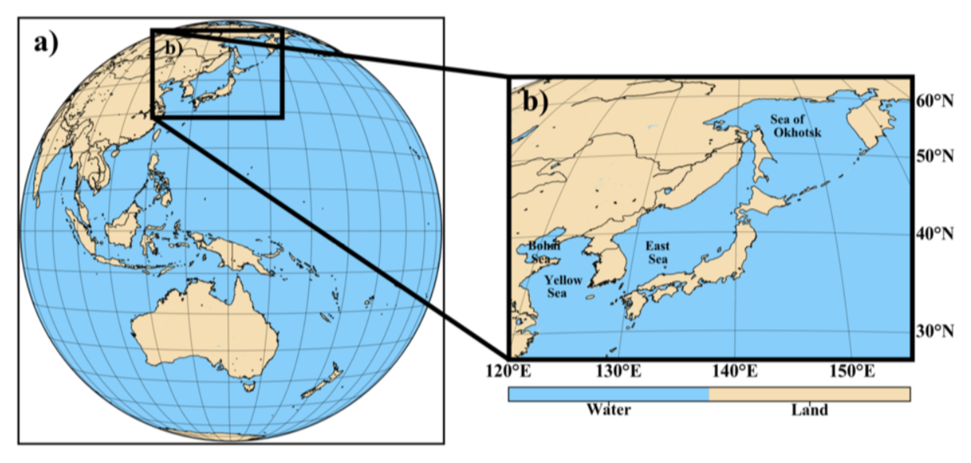
2.1. Study Area
2.2. Satellite Data
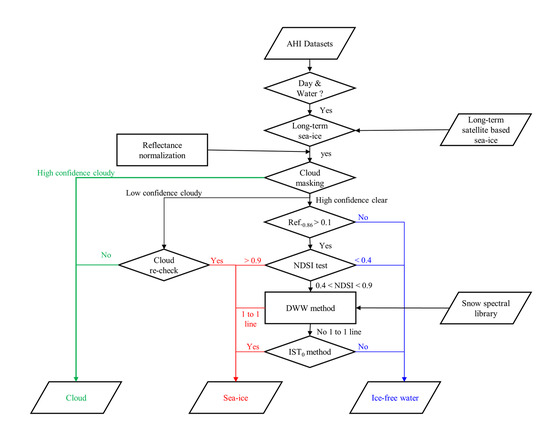
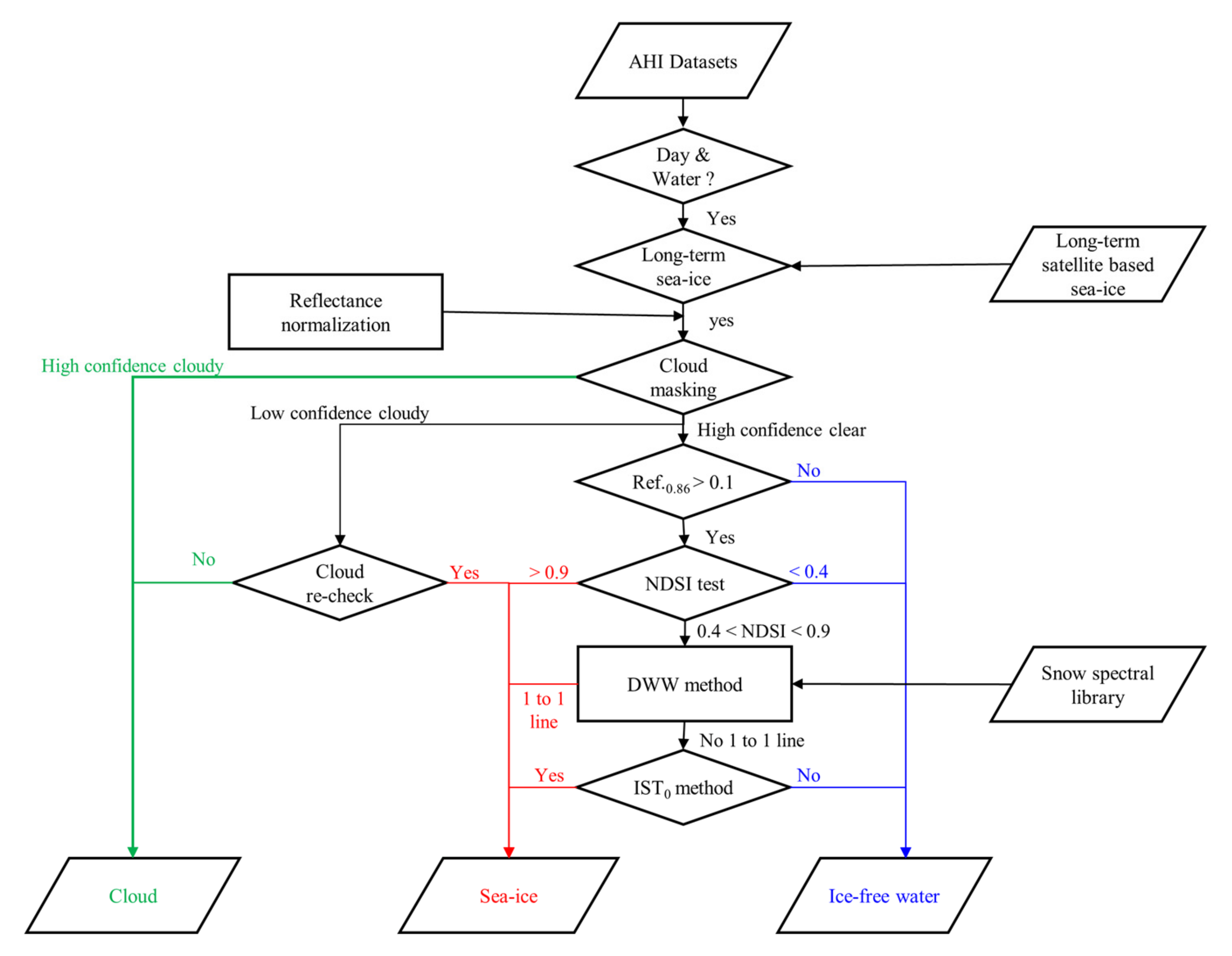
3. Sea-ice Detection Algorithm
- Preprocessing of data and identification of potential sea ice areas;
- Sea ice detection under clear skies; high confidence clear on GK-2A/AMI cloud mask;
- Sea ice detection for the low-confidence cloudy, which is classified using the GK-2A/AMI cloud mask.
4. Validation Results of GK-2A/AMI Sea-Ice Detection Algorithm
4.1. Comparison/Validation Method
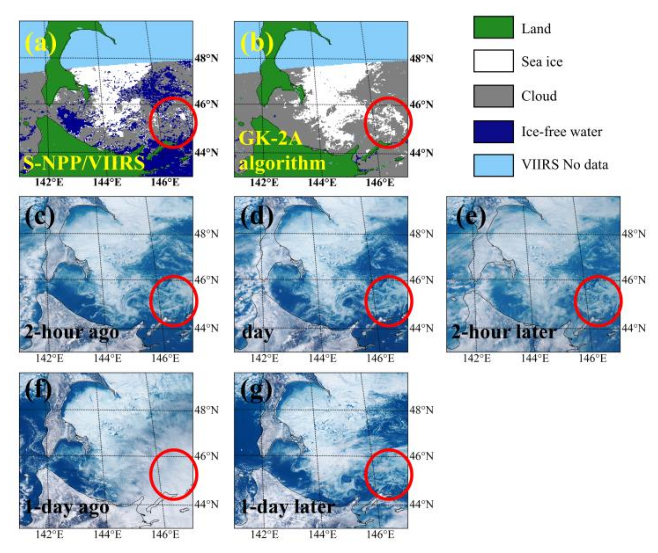
4.2. Comparison with S-NPP/VIIRS Sea-Ice Characterization Environmental Data Record
4.3. Performance with Sea-Ice ROI Data
5. Discussion and Conclusions
Author Contributions
Funding
Acknowledgments
Conflicts of Interest
References
- Ledley, T.S. A coupled energy balance climate-sea ice model: Impact of sea ice and leads on climate. J. Geophys. Res. Atmos. 1988, 93, 15919–15932. [Google Scholar] [CrossRef]
- Cavalieri, D.J.; Parkinson, C.L. Arctic sea ice variability and trends, 1979–2010. Cryosphere 2012, 5, 881. [Google Scholar] [CrossRef] [Green Version]
- Meier, W.N.; Markus, T.; Comiso, J.; Ivanoff, A.; Miller, J. AMSR2 Sea Ice Algorithm Theoretical Basis Document; NASA Goddard Space Flight Center: Greenbelt, MD, USA, 2017. [Google Scholar]
- Hall, D.K.; Riggs, G.A.; Salomonson, V.V.; Barton, J.S.; Casey, K.; Chien, J.Y.L.; DiGirolamo, N.E.; Klein, A.G.; Powell, H.W.; Tait, A.B. Algorithm Theoretical Basis Document (ATBD) for the MODIS Snow and Sea Ice-Mapping Algorithms; NASA Goddard Space Flight Center: Greenbelt, MD, USA, 2001; Volume 45. [Google Scholar]
- Baker, N. Joint Polar Satellite System (JPSS) VIIRS Sea Ice Characterization Algorithm Theoretical Basis Document (ATBD); NASA Goddard Space Flight Center Green belt; NASA Goddard Space Flight Center: Greenbelt, MD, USA, 2011. [Google Scholar]
- Liu, Y.; Key, J.R. Algorithm Theoretical Basis Document (ATBD); Ice Surface Temperature, Ice Concentration and Ice Cover; NOAA Nesdis Center for Satellite Applications and Research: Silver Spring, MD, USA, 2019. [Google Scholar]
- Ioka, Y.; Yogo, Y.; Tanikawa, T.; Hosaka, M.; Ishida, H.; Aoki, T. Algorithm Theoretical Basis for the Himawari-8,-9/AHI Cryosphere Product Part 2: Sea Ice Distribution. Meteorol. Satell. Cent. Tech. Note 2019, 64, 13–21. [Google Scholar]
- Ludwig, V.; Spreen, G.; Haas, C.; Istomina, L.; Kauker, F.; Murashkin, D. The 2018 North Greenland polynya observed by a newly introduced merged optical and passive microwave sea-ice concentration dataset. Cryosphere 2019, 13, 2051–2073. [Google Scholar] [CrossRef] [Green Version]
- Zakhvatkina, N.; Smirnov, V.; Bychkova, I. Satellite sar data-based sea ice classification: An overview. Geosciences 2019, 9, 152. [Google Scholar] [CrossRef] [Green Version]
- Temimi, M.; Romanov, P.; Ghedira, H.; Khanbilvardi, R.; Smith, K. Sea-ice monitoring over the Caspian Sea using geostationary satellite data. Int. J. Remote Sens. 2011, 32, 1575–1593. [Google Scholar] [CrossRef]
- Gerland, S.; Barber, D.; Meier, W.; Mundy, C.J.; Holland, M.; Kern, S.; Li, Z.; Michel, C.; Perovich, D.K.; Tamura, T. Essential gaps and uncertainties in the understanding of the roles and functions of Arctic sea ice. Environ. Res. Lett. 2019, 14, 043002. [Google Scholar] [CrossRef]
- Seong, N.H.; Jung, D.; Kim, J.; Han, K.S. Evaluation of NDVI Estimation Considering Atmospheric and BRDF Correction through Himawari-8/AHI. Asia Pac. J. Atmos. Sci. 2020, 5, 1–10. [Google Scholar] [CrossRef] [Green Version]
- Lee, K.S.; Lee, C.S.; Seo, M.; Choi, S.; Seong, N.H.; Jin, D.; Yeom, J.M.; Han, K.S. Improvements of 6S Look-Up-Table Based Surface Reflectance Employing Minimum Curvature Surface Method. Asia Pac. J. Atmos. Sci. 2020, 3, 1–14. [Google Scholar] [CrossRef] [Green Version]
- Choi, Y.Y.; Suh, M.S. Development of Himawari-8/Advanced Himawari Imager (AHI) land surface temperature retrieval algorithm. Remote Sens. 2018, 10, 2013. [Google Scholar] [CrossRef] [Green Version]
- Lee, S.J.; Ahn, M.H.; Chung, S.R. Atmospheric profile retrieval algorithm for next generation geostationary satellite of Korea and its application to the advanced Himawari Imager. Remote Sens. 2017, 9, 1294. [Google Scholar] [CrossRef] [Green Version]
- Lee, S.H.; Kim, B.Y.; Lee, K.T.; Zo, I.S.; Jung, H.S.; Rim, S.H. Retrieval of reflected shortwave radiation at the top of the atmosphere using Himawari-8/AHI data. Remote Sens. 2018, 10, 213. [Google Scholar] [CrossRef] [Green Version]
- Oh, S.M.; Borde, R.; Carranza, M.; Shin, I.C. Development and Intercomparison Study of an Atmospheric Motion Vector Retrieval Algorithm for GEO-KOMPSAT-2A. Remote Sens. 2019, 11, 2054. [Google Scholar] [CrossRef] [Green Version]
- Imai, T.; Yoshida, R. Algorithm theoretical basis for Himawari-8 cloud mask product. Meteorol. Satell. Cent. Tech. Note 2016, 61, 1–17. [Google Scholar]
- Key, J.R.; Mahoney, R.; Liu, Y.; Romanov, P.; Tschudi, M.; Appel, I.; Maslanik, J.; Baldwin, D.; Wang, X.; Meade, P. Snow and ice products from Suomi NPP VIIRS. J. Geophys. Res. Atmos. 2013, 118. [Google Scholar] [CrossRef]
- Ning, L.; Xie, F.; Gu, W.; Xu, Y.; Huang, S.; Yuan, S.; Cui, W.; Levy, J. Using remote sensing to estimate sea ice thickness in the Bohai Sea, China based on ice type. Int. J. Remote Sens. 2009, 30, 4539–4552. [Google Scholar] [CrossRef]
- Key, J.R.; Wang, X.; Stoeve, J.C.; Fowler, C. Estimating the cloudy-sky albedo of sea ice and snow from space. J. Geophys. Res. Atmos. 2001, 106, 12489–12497. [Google Scholar] [CrossRef] [Green Version]
- Mundy, C.J.; Barber, D.G.; Michel, C. Variability of snow and ice thermal, physical and optical properties pertinent to sea ice algae biomass during spring. J. Mar. Syst. 2005, 58, 107–120. [Google Scholar] [CrossRef]
- Nazari, R.; Khanbilvardi, R. Application of dynamic threshold in sea and lake ice mapping and monitoring. Int. J. Hydrol. Sci. Technol. 2011, 1, 37–46. [Google Scholar] [CrossRef]
- Warren, S.G. Optical properties of snow. Rev. Geophys. 1982, 20, 67. [Google Scholar] [CrossRef]
- Cline, D.; Rost, A.; Painter, T.; Bovitz, C. Algorithm Theoretical Basis Document (ATBD); Snow Cover; NOAA Nesdis Center for Satellite Applications and Research: Silver Spring, MD, USA, 2010. [Google Scholar]
- Xin, Q.; Woodcock, C.E.; Liu, J.; Tan, B.; Melloh, R.A.; Davis, R.E. View angle effects on MODIS snow mapping in forests. Remote Sens. Environ. 2012, 118, 50–59. [Google Scholar] [CrossRef] [Green Version]
- Key, J.R.; Collins, J.B.; Fowler, C.; Stone, R.S. High-latitude surface temperature estimates from thermal satellite data. Remote Sens. Environ. 1997, 61, 302–309. [Google Scholar] [CrossRef]
- Yan, Y.; Huang, K.; Shao, D.; Xu, Y.; Gu, W. Monitoring the Characteristics of the Bohai Sea Ice Using High-Resolution Geostationary Ocean Color Imager (GOCI) Data. Sustainability 2019, 11, 777. [Google Scholar] [CrossRef] [Green Version]
- Miao, X.; Xie, H.; Ackley, S.F.; Perovich, D.K.; Ke, C. Object-based detection of Arctic sea ice and melt ponds using high spatial resolution aerial photographs. Cold Reg. Sci. Technol. 2015, 119, 211–222. [Google Scholar] [CrossRef]
- Zhang, N.; Ma, Y.; Zhang, Q. Prediction of sea ice evolution in Liaodong Bay based on a back-propagation neural network model. Cold Reg. Sci. Technol. 2018, 145, 65–75. [Google Scholar] [CrossRef]
- Honda, M.; Yamazaki, K.; Nakamura, H.; Takeuchi, K. Dynamic and thermodynamic characteristics of atmospheric response to anomalous sea-ice extent in the Sea of Okhotsk. J. Clim. 1999, 12, 3347–3358. [Google Scholar] [CrossRef]
- Minervin, I.G.; Romanyuk, V.A.E.; Pishchal’nik, V.M.; Truskov, P.A.E.; Pokrashenko, S.A. Zoning the ice cover of the Sea of Okhotsk and the Sea of Japan. Her. Russ. Acad. Sci. 2015, 85, 132–139. [Google Scholar] [CrossRef]
- Wakabayashi, H.; Mori, Y.; Nakamura, K. Sea ice detection in the sea of Okhotsk using PALSAR and MODIS data. IEEE J. Sel. Top. Appl. Earth Obs. Remote Sens. 2013, 6, 1516–1523. [Google Scholar] [CrossRef]
- Nihashi, S.; Kurtz, N.T.; Markus, T.; Ohshima, K.I.; Tateyama, K.; Toyota, T. Estimation of sea-ice thickness and volume in the Sea of Okhotsk based on ICESat data. Ann. Glaciol. 2018, 59, 101–111. [Google Scholar] [CrossRef] [Green Version]
- Toyota, T.; Baba, K.; Hashiya, E.; Ohshima, K.I. In-situ ice and meteorological observations in the southern Sea of Khotsk in 2001 winter: Ice structure, snow on ice, surface temperature, and optical environments. Polar Meteorol. Glaciol. 2002, 16, 116–132. [Google Scholar]
- Shi, W.; Wang, M. Sea ice properties in the Bohai Sea measured by MODIS-Aqua: 1. Satellite algorithm development. J. Mar. Syst. 2012, 95, 32–40. [Google Scholar] [CrossRef]
- Su, H.; Wang, Y.; Yang, J. Monitoring the spatiotemporal evolution of sea ice in the Bohai Sea in the 2009–2010 winter combining MODIS and meteorological data. Estuaries Coasts 2012, 35, 281–291. [Google Scholar] [CrossRef] [Green Version]
- Karvonen, J.; Shi, L.; Cheng, B.; Similä, M.; Mäkynen, M.; Vihma, T. Bohai Sea ice parameter estimation based on thermodynamic ice model and Earth observation data. Remote Sens. 2017, 9, 234. [Google Scholar] [CrossRef] [Green Version]
- Yan, Y.; Shao, D.; Gu, W.; Liu, C.; Li, Q.; Chao, J.; Tao, J.; Xu, Y. Multidecadal anomalies of Bohai Sea ice cover and potential climate driving factors during 1988–2015. Environ. Res. Lett. 2017, 12, 094014. [Google Scholar] [CrossRef]
- Yan, Y.; Uotila, P.; Huang, K.; Gu, W. Variability of sea ice area in the Bohai Sea from 1958 to 2015. Sci. Total Environ. 2020, 709, 136164. [Google Scholar] [CrossRef]
- Su, H.; Ji, B.; Wang, Y. Sea Ice Extent Detection in the Bohai Sea Using Sentinel-3 OLCI Data. Remote Sens. 2019, 11, 2436. [Google Scholar] [CrossRef] [Green Version]
- NMSC: GK-2A AMI Algorithm Theoretical Basis Document. Available online: http://nmsc.kma.go.kr/homepage/html/base/cmm/selectPage.do?page=static.edu.atbdGk2a (accessed on 15 April 2019).
- Murata, K.T.; Pavarangkoon, P.; Higuchi, A.; Toyoshima, K.; Yamamoto, K.; Muranaga, K.; Nagaya, Y.; Izumikawa, Y.; Kimura, E.; Mizuhara, T. A web-based real-time and full-resolution data visualization for Himawari-8 satellite sensed images. Earth Sci. Inform. 2018, 11, 217–237. [Google Scholar] [CrossRef] [Green Version]
- Riggs, G.A.; Hall, D.K.; Salomonson, V.V. MODIS Sea Ice Products User Guide to Collection 5; NASA Goddard Space Flight Center: Greenbelt, MD, USA, 2006; Volume 49. [Google Scholar]
- Hall, D.K.; Key, J.R.; Casey, K.A.; Riggs, G.A.; Cavalieri, D.J. Sea ice surface temperature product from the Moderate Resolution Imaging Spectroradiometer (MODIS). IEEE Trans. Geosci. Remote Sens. 2004, 42, 1076–1087. [Google Scholar] [CrossRef]
- Shuman, C.A.; Hall, D.K.; DiGirolamo, N.E.; Mefford, T.K.; Schnaubelt, M.J. Comparison of near-surface air temperatures and MODIS ice-surface temperatures at Summit, Greenland (2008–13). J. Appl. Meteorol. 2014, 53, 2171–2180. [Google Scholar] [CrossRef]
- Scambos, T.A.; Haran, T.M.; Massom, R. Validation of AVHRR and MODIS ice surface temperature products using in situ radiometers. Ann. Glaciol. 2006, 44, 345–351. [Google Scholar] [CrossRef] [Green Version]
- Rösel, A.; Kaleschke, L.; Birnbaum, G. Melt ponds on Arctic sea ice determined from MODIS satellite data using an artificial neural network. Cryosphere 2012, 6, 431–446. [Google Scholar] [CrossRef] [Green Version]
- Mäkynen, M.; Karvonen, J. MODIS sea ice thickness and open water–sea ice charts over the Barents and Kara Seas for development and validation of sea ice products from microwave sensor data. Remote Sens. 2017, 9, 1324. [Google Scholar] [CrossRef] [Green Version]
- Hall, D.K.; Riggs, G.A. Accuracy assessment of the MODIS snow products. Hydrol. Process. 2007, 21, 1534–1547. [Google Scholar] [CrossRef]
- Huang, X.; Liang, T.; Zhang, X.; Guo, Z. Validation of MODIS snow cover products using Landsat and ground measurements during the 2001–2005 snow seasons over northern Xinjiang, China. Int. J. Remote Sens. 2011, 32, 133–152. [Google Scholar] [CrossRef]
- Hall, D.K.; Foster, J.L.; Verbyla, D.L.; Klein, A.G.; Benson, C.S. Assessment of snow-cover mapping accuracy in a variety of vegetation-cover densities in central Alaska. Remote Sens. Environ. 1998, 66, 129–137. [Google Scholar] [CrossRef]
- Wang, X.; Xie, H.; Liang, T. Evaluation of MODIS snow cover and cloud mask and its application in Northern Xinjiang, China. Remote Sens. Environ. 2008, 112, 1497–1513. [Google Scholar] [CrossRef]
- Maskey, S.; Uhlenbrook, S.; Ojha, S. An analysis of snow cover changes in the Himalayan region using MODIS snow products and in-situ temperature data. Clim. Chang. 2011, 108, 391. [Google Scholar] [CrossRef]
- Rikiishi, K.; Hashiya, E.; Imai, M. Linear trends of the length of snow-cover season in the Northern Hemisphere as observed by the satellites in the period 1972–2000. Ann. Glaciol. 2004, 38, 229–237. [Google Scholar] [CrossRef] [Green Version]
- Estilow, T.W.; Young, A.H.; Robinson, D.A. A long-term Northern Hemisphere snow cover extent data record for climate studies and monitoring. Earth Syst. Sci. Data 2015, 7, 137. [Google Scholar] [CrossRef] [Green Version]
- Romanov, P. Global multisensor automated satellite-based snow and ice mapping system (GMASI) for cryosphere monitoring. Remote Sens. Environ. 2017, 196, 42–55. [Google Scholar] [CrossRef]
- Lee, K.S.; Jin, D.; Yeom, J.M.; Seo, M.; Choi, S.; Kim, J.J.; Han, K.S. New Approach for Snow Cover Detection through Spectral Pattern Recognition with MODIS Data. J. Sensors 2017. [Google Scholar] [CrossRef]
- Gignac, C.; Bernier, M.; Chokmani, K.; Poulin, J. IceMap250—Automatic 250 m sea ice extent mapping using MODIS data. Remote Sens. 2017, 9, 70. [Google Scholar] [CrossRef] [Green Version]
- Thoss, A. Algorithm Theoretical Basis Document for SAF NWC/PPS “Cloud Mask”(CM-PGE01 v. 3.0, patch 1) (No. 2.3, p. 48). SAF/NWC/CDOP/SMHI-PPS/SCI/ATBD/1. 2010. Available online: http://www.nwcsaf.org/AemetWebContents/ScientificDocumentation/Documentation/PPS/v2014/NWC-CDOP2-PPS-SMHI-SCI-ATBD-1_v1_0.pdf (accessed on 13 July 2020).
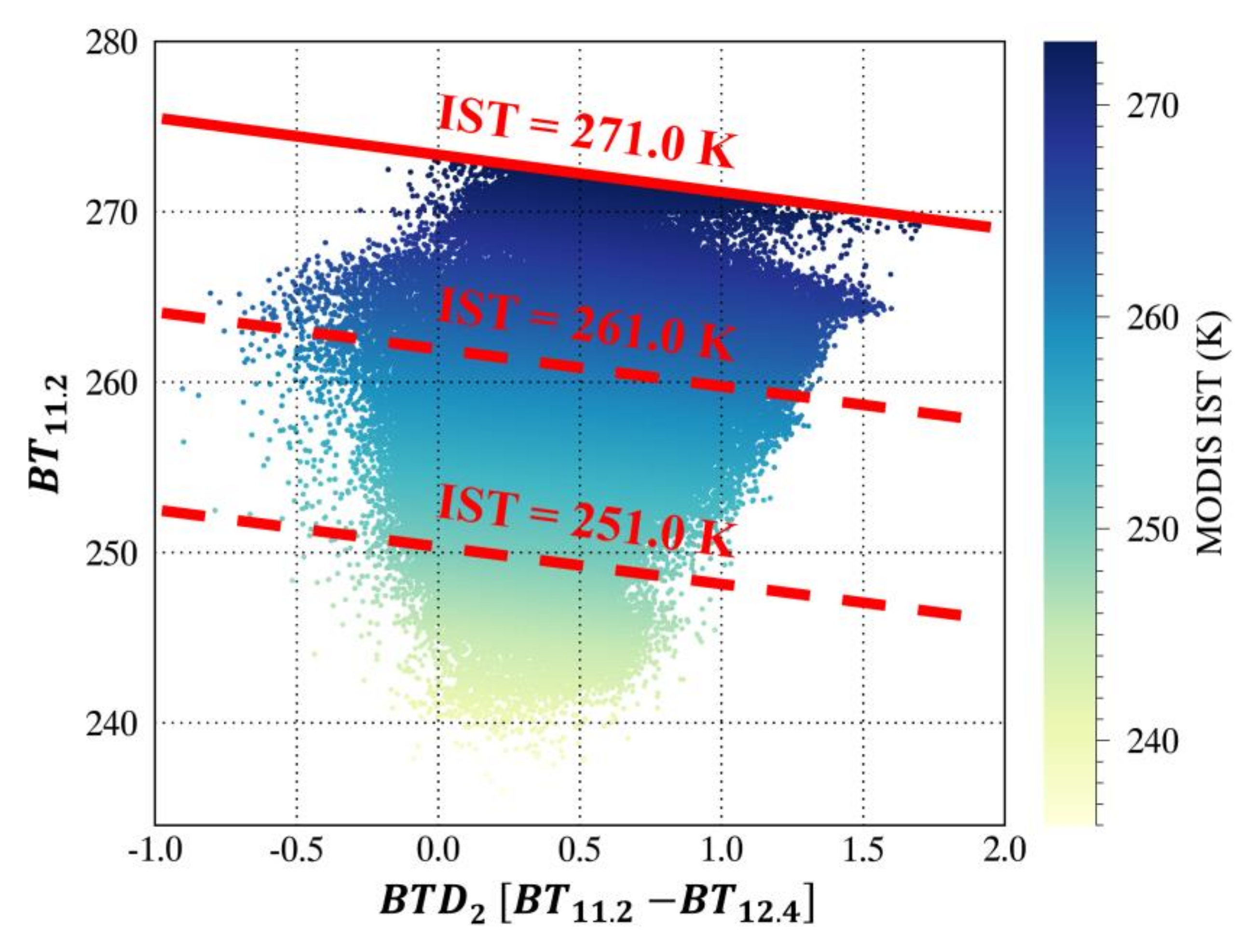
- Jin, D.; Lee, K.S.; Choi, S.; Seo, M.; Lee, D.; Kwon, C.; Kim, H.; Lee, E.K.; Han, K.S. Determination of dynamic threshold for sea-ice detection through relationship between 11 μm brightness temperature and 11–12 μm brightness temperature difference. Korean J. Remote Sens. 2017, 33, 243–248. [Google Scholar]
- Siljamo, N.; Hyvärinen, O. New Geostationary Satellite–Based Snow-Cover Algorithm. J. Appl. Meteorol. 2011, 50, 1275–1290. [Google Scholar] [CrossRef]
- Chaouch, N.; Temimi, M.; Romanov, P.; Cabrera, R.; McKillop, G.; Khanbilvardi, R. An automated algorithm for river ice monitoring over the Susquehanna River using the MODIS data. Hydrol. Process. 2014, 28, 62–73. [Google Scholar] [CrossRef]
- Gerhardinger, A.; Ehrlich, D.; Pesaresi, M. Vehicles detection from very high resolution satellite imagery. Int. Arch. Photogramm. Remote Sens. 2015, 36, W24. [Google Scholar]
- Baumstark, R.; Duffey, R.; Pu, R. Mapping seagrass and colonized hard bottom in Springs Coast, Florida using WorldView-2 satellite imagery. Estuar. Coast. Shelf Sci. 2016, 181, 83–92. [Google Scholar] [CrossRef]
- Inglada, J.; Vincent, A.; Arias, M.; Tardy, B.; Morin, D.; Rodes, I. Operational high resolution land cover map production at the country scale using satellite image time series. Remote Sens. 2017, 9, 95. [Google Scholar] [CrossRef] [Green Version]
- Hall, D.K.; Riggs, G.A.; Salomonson, V.V.; DiGirolamo, N.E.; Bayr, K.J. MODIS snow-cover products. Remote Sens. Environ. 2002, 83, 181–194. [Google Scholar] [CrossRef] [Green Version]
- Hutchison, K.D.; Iisager, B.D.; Mahoney, R.L. Enhanced snow and ice identification with the VIIRS cloud mask algorithm. Remote Sens. Lett. 2013, 4, 929–936. [Google Scholar] [CrossRef]
- Louis, J.; Devignot, O.; Pessiot, L. S2 MPC–L2A Product Definition Document. Ref. S2-PDGS-MPC-L2A-PDD-V14, 2(4.6). 2018. Available online: https://sentinel.esa.int/documents/247904/685211/S2+L2A+Product+Definition+Document/2c0f6d5f-60b5-48de-bc0d-e0f45ca06304 (accessed on 11 July 2020).


| GK-2A/AMI Sea-Ice Detection Algorithm | Comparison/Validation Data | |
|---|---|---|
| Sea Ice | Ice-Free Water | |
| Sea ice | Hit (a) | False (b) |
| Ice-free water | Miss (c) | Correct rejection (d) |
| YYYYMMDD.hhmn (S-NPP/VIIRS Time) | GK-2A/AMI Sea-Ice Detection Algorithm | S-NPP/VIIRS SIC EDR | ||
|---|---|---|---|---|
| POD/FAR (%) | OA (%) | POD/FAR (%) | OA (%) | |
| 20180112.0140 (0142) | 98.35/0.00 | 98.35 | 61.48/0.00 | 61.48 |
| 20180116.0200 (0203) | 98.01/0.00 | 98.11 | 97.85/0.00 | 97.96 |
| 20180116.0350 (0345) | 98.81/0.00 | 98.82 | 95.51/0.00 | 95.53 |
| 20180203.0310 (0309) | 94.70/0.00 | 94.70 | 99.23/0.00 | 99.23 |
| 20180203.0450 (0451) | 98.73/0.00 | 98.73 | 97.96/0.00 | 97.96 |
| 20180204.0250 (0246) | 94.15/0.00 | 95.70 | 98.52/0.00 | 98.90 |
| 20180204.0250 (0252) | 95.97/0.00 | 95.97 | 99.87/0.00 | 99.87 |
| 20180216.0400 (0400) | 99.70/0.00 | 99.89 | 98.18/0.00 | 99.34 |
| 20180220.0250 (0250) | 96.14/0.00 | 96.14 | 98.37/0.00 | 98.34 |
| 20180311.0330 (0333) | 93.85/0.00 | 94.06 | 88.48/0.00 | 88.87 |
| Total | 96.54/0.00 | 97.23 | 96.00/0.00 | 96.81 |
© 2020 by the authors. Licensee MDPI, Basel, Switzerland. This article is an open access article distributed under the terms and conditions of the Creative Commons Attribution (CC BY) license (http://creativecommons.org/licenses/by/4.0/).
Share and Cite
Jin, D.; Chung, S.-R.; Lee, K.-S.; Seo, M.; Choi, S.; Seong, N.-H.; Jung, D.; Sim, S.; Kim, J.; Han, K.-S. Development of Geo-KOMPSAT-2A Algorithm for Sea-Ice Detection Using Himawari-8/AHI Data. Remote Sens. 2020, 12, 2262. https://doi.org/10.3390/rs12142262
Jin D, Chung S-R, Lee K-S, Seo M, Choi S, Seong N-H, Jung D, Sim S, Kim J, Han K-S. Development of Geo-KOMPSAT-2A Algorithm for Sea-Ice Detection Using Himawari-8/AHI Data. Remote Sensing. 2020; 12(14):2262. https://doi.org/10.3390/rs12142262
Chicago/Turabian StyleJin, Donghyun, Sung-Rae Chung, Kyeong-Sang Lee, Minji Seo, Sungwon Choi, Noh-Hun Seong, Daeseong Jung, Suyoung Sim, Jinsoo Kim, and Kyung-Soo Han. 2020. "Development of Geo-KOMPSAT-2A Algorithm for Sea-Ice Detection Using Himawari-8/AHI Data" Remote Sensing 12, no. 14: 2262. https://doi.org/10.3390/rs12142262