Determination of Planetary Boundary Layer height with Lidar Signals Using Maximum Limited Height Initialization and Range Restriction (MLHI-RR)

Abstract

The planetary boundary layer height (PBLH) is a vital parameter to characterize the surface convection, which determines the diffusion of air pollutants. The accurate inversion of PBLH is extremely important for the study of aerosol concentrations, in order to predict air quality and provide weather forecast. Aerosol lidar, a powerful remote sensing instrument for detecting the characteristics of atmospheric temporal and spatial evolution, can continuously retrieve the planetary boundary layer (PBL) and obtain high resolution measurements. However, multi-layer conditions, including one or more layers of aerosol, or cloud above the PBL, can seriously interfere the accuracy of PBLH determined by lidar. A new technique of maximum limited height initialization and range restriction (MLHI-RR) is proposed to eliminate the impact of multi-layer conditions on PBLH determination. Four widely used methods for deriving PBLH are utilized, in addition to the MLHI-RR constraint. Comparisons demonstrate that the proposed technique can determine the PBLH in multi-layer conditions with higher accuracy. The proposed technique requires no affiliate information besides lidar signals, which provide a convenient method for PBLH determination under complicated conditions.

1. Introduction

The planetary boundary layer (PBL) refers to the turbulent mixing layer closest to the Earth’s surface, and it is directly affected by the convective fluxes. It is the direct receptor of pollutants emitted by human activities, with a response time scale of an hour or less [1]. The exchanges of momentum, heat, moisture, natural and anthropogenic chemical constituents take place between the free atmosphere and surface through the PBL [2]. This work mainly considers the cases in neutral and unstable conditions of PBL. The unstable boundary layer is also referred to as the mixing layer under this circumstance [3]. The aerosol distribution within the mixing layer is usually well mixed and, thus, it is assumed to be uniform in this work.

The PBL height (PBLH) is the height at the top of the PBL. The PBLH determines many tropospheric processes related to air pollution, including convective activity, aerosol distributions, cloud and fog formation. As a result, PBLH has been used as a key parameter in weather, climate and air quality models, to determine turbulence mixing, vertical diffusion, convective transport, cloud/aerosol entrainment and atmospheric pollutant deposition [4,5]. Consequently, the detection of the PBLH has always been an important research direction. The methods of the PBLH determination can be roughly divided into two categories: in situ and remote sensing measurements. In situ observations are to carry out contact measurement of atmospheric parameters by means of radio soundings (radiosonde, tethered balloon, aircraft) and retrieve the PBLH from the vertical profiles of atmospheric parameters [6,7,8]. Although in situ techniques can provide vertical profiles of meteorological elements, they have major disadvantages of sparse spatial coverage and infrequent observation. In recent years, remote sensing instruments (sodars, wind profiling radars, lidars) are a more efficient way for a continuous PBL top detection [9,10,11].

Lidar, a powerful active remote sensing instrument, has the advanced abilities of strong operability, continuous observation and high spatial-temporal resolution in aerosol [12,13,14]. Tang et al. [15] observed the PBLH in Beijing from July 2009 to December 2012 using a ceilometer, and presented that the dissipation of atmospheric particles mainly depends on the PBLH. Erica et al. [16] estimated summertime PBLH over North America derived from space-borne lidar in 2012, finding that PBLH can improve the understanding of the exchange process of energy and matter between the surface and the atmosphere. In 2016, Gregori et al. [17] compared and analyzed the PBLH determined by microwave radiometer, elastic lidar and Doppler lidar, showing that the inversion results based on active remote sensing are consistent in most cases.

However, the complexity of atmospheric structure challenges the accurate identification of PBLH. The most important and challenging part is to find the true PBLH when several local minima in signal gradients appear on the profiles under the influence of elevated aerosols or clouds above the PBL [18]. Several widely used techniques [19,20], such as the gradient method (GM) [21], the curve fitting method (CFM) [22], the wavelet covariance transform method (WCT) [23] and the standard deviation method (STD) [24] of lidar to estimate the PBLH from lidar backscatter signals are unable to obtain the true PBLH anymore. For example, in the case of clouds, the strong attenuation of lidar backscatter signals at the upper edge of clouds is similar to that at the top of PBL, which leads to the ambiguity over whether the height retrieved by lidar method is true or not [25]. Toledo et al. [26] analyzed six commonly used methods of measuring PBLH by lidar, and presented that, when residual layers appear in the measurement, there is a large discrepancy between the PBLH detected by lidar and that detected by radio soundings. Thus, it is crucial to consider the influence of lofted aerosol layers or clouds above the PBL for PBLH inversion based on lidar backscatter signals. Certainly, many improved technologies have been studied and put forward to overcome this difficulty [27,28,29], but these methods are generally used to eliminate one specific influence among elevated aerosols, residual layers or clouds. Actually, in continuous variations of the PBL, these influences are frequently mixed and occurred simultaneously. Moreover, the subjective or empirical threshold obtained at one location may not be applicable for other geological locations with different PBL structures. Hence, we develop a method that can eliminate the multi-layer conditions effect and is generally applicable.

In this paper, a technique is proposed to eliminate the interference of aloft aerosol layers and clouds on the PBLH determination merely depended on lidar data. Therefore, the veracity of PBLH retrieval only relies on the accuracy of lidar observations and the characteristics of the retrieving methods. The technique is inferred to as the maximum limited height initialization and range restriction (MLHI-RR) method in following text. The lidar data from University of Wisconsin (http://hsrl.ssec.wisc.edu/) database is employed. The MLHI-RR are initializing the maximum limited height in the first short period of time (T+ΔT) by utilizing the volume backscatter coefficient of aerosols and determining the range restriction with the moving window algorithm using the PBLH in this period of time. With consideration of the temporal continuity, the first step of the MLHI-RR technique employs four independent methods to determine the PBLH within a small portion of the profiles. Next, the MLHI-RR technique retrieves the PBLH of the remaining profiles under multi-layer conditions with a constraint of height difference from the obtained PBLH. The results are assessed by comparison with the PBLH retrieved from the temperature-gradient method, on the basis of vertical temperature profile from a nearby radiosonde site. A comparison experiment demonstrates that the MLHI-RR algorithm is more stable in determining the PBLH, compared with no limiter under multi-layer conditions. In particular, measurements of continuous variations in PBLH indicate that the new technique not only possesses better feasibility than traditional methods, but also maintains comparable stability.

The remainder of paper is organized as follows. In Section 2, the principle of lidar detecting PBLH and the method of determining PBLH are described. A new technique to eliminate the interference of lofted aerosol layers and clouds is introduced in Section 3. Section 4 presents result analysis and discussion including the comparison of the lidar and radiosonde measurements of PBLH, and the variations in PBLH with elevated aerosols and clouds. A short summary is given in Section 5. The abbreviation index of proper nouns used in this paper is shown in

Table A1. Abbreviation Index.

Abbreviation	Whole Words
PBL	planetary boundary layer
PBLH	planetary boundary layer height
MLHI-RR	maximum limited height initialization and range restriction
MLH	maximum limited height
RR	range restriction
GM	gradient method
CFM	curve fitting method
WCT	wavelet covariance transform method
STD	standard deviation method
LT	local time
AGL	above ground level
RCS	range-corrected signal

of the Appendix A.

2. The Principle of Lidar PBLH Detection

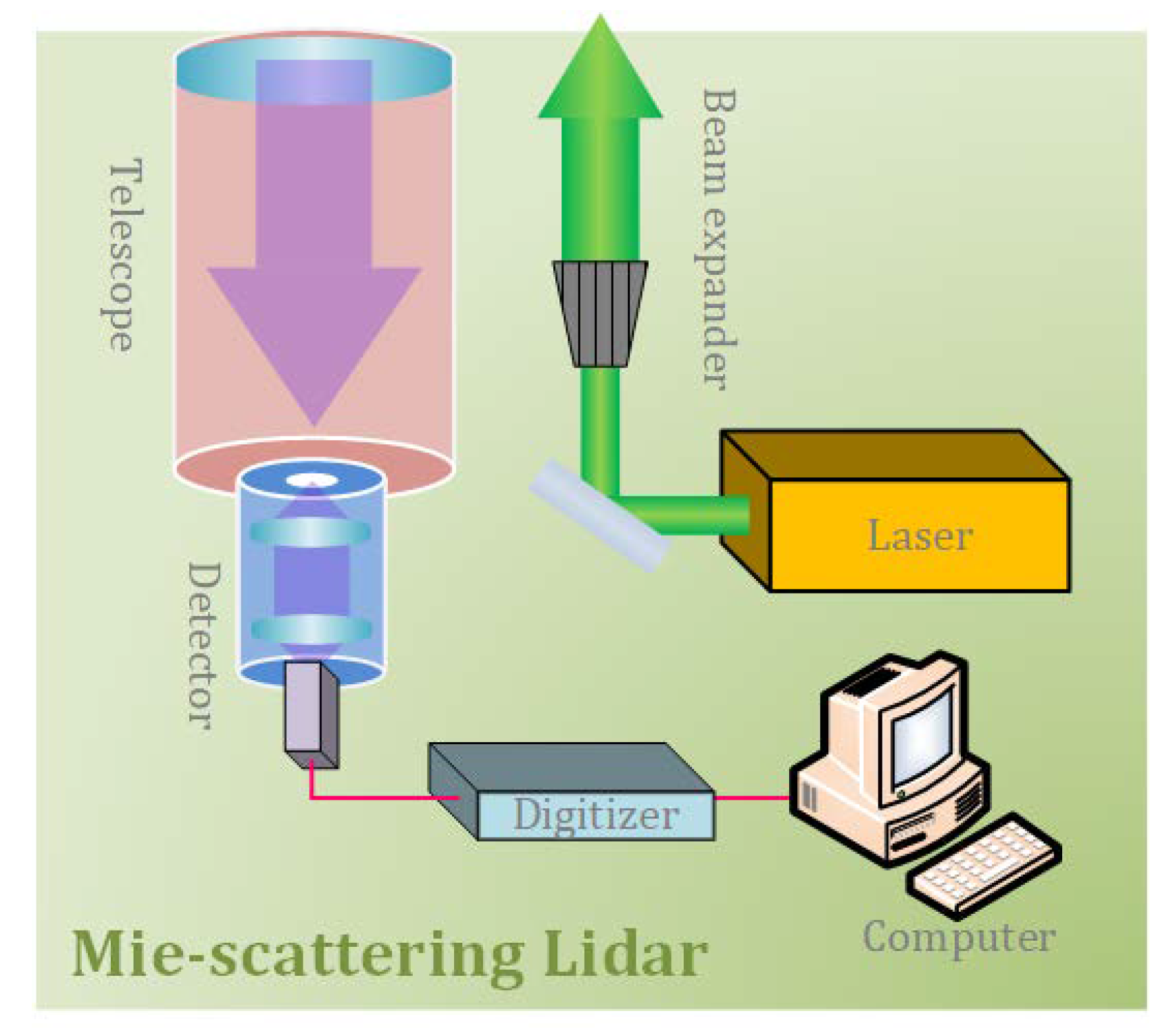
2.1. A Mie-Scattering Lidar

The height up to which sensible heat is transported is denoted by the PBLH. Since passive scalars are accumulated in the PBL and, therefore, a large gradient of aerosol concentration occurs at the inversion capping the PBL, this means that this gradient is also suited for defining the top of the PBL. Owing to the existence of inversion layer, a large number of aerosol particles are bound below the inversion layer, while in the free atmosphere above the inversion layer, the concentration of aerosol particles is sparse. The lidar echo signal intensity is directly related to the aerosol concentration at certain altitude. When the laser beam passes through the boundary between the PBL and the free atmosphere, it will be severely attenuated. Therefore, the abrupt change of the echo signal intensity can be used to determine the PBLH. A Mie-scattering lidar was employed for this study and its sketch is shown in Figure 1, which mainly includes the laser emission component, the telescope receiving component, the photoelectric conversion component, as well as the data acquisition and processing component [30,31]. A Mie-scattering lidar emits high-energy laser pulses to the atmosphere, which then collects the light signals from aerosol backscattering with telescope, and calculates the aerosol parameters according to a certain inversion model. The lidar signal can be expressed as

$$P\left(R\right)=\frac{C}{R^2}\beta \left(R\right)\exp \left[-2{\displaystyle {\int }_0^R\alpha \left(R\right)dR}\right]$$

(1)

where C is a system constant for a given lidar, R is the detection height, β is the backscatter coefficient and α is the extinction coefficient. β is calculated according to the Fernald method by assuming the lidar ratio and boundary value of the aerosol [32,33]. The backscatter coefficient has a certain deviation retrieved from Fernald method. Fortunately, there are many improved algorithms, which can reduce the deviation and get more accurate backscatter coefficient [34]. Range-corrected signal (RCS) is defined as: $X\left(R\right)=P\left(R\right)R^2$. The change of RCS with height indicates the change of aerosol concentrations and the four variety lidar methods used to determine the PBLH in this paper are based on RCS.

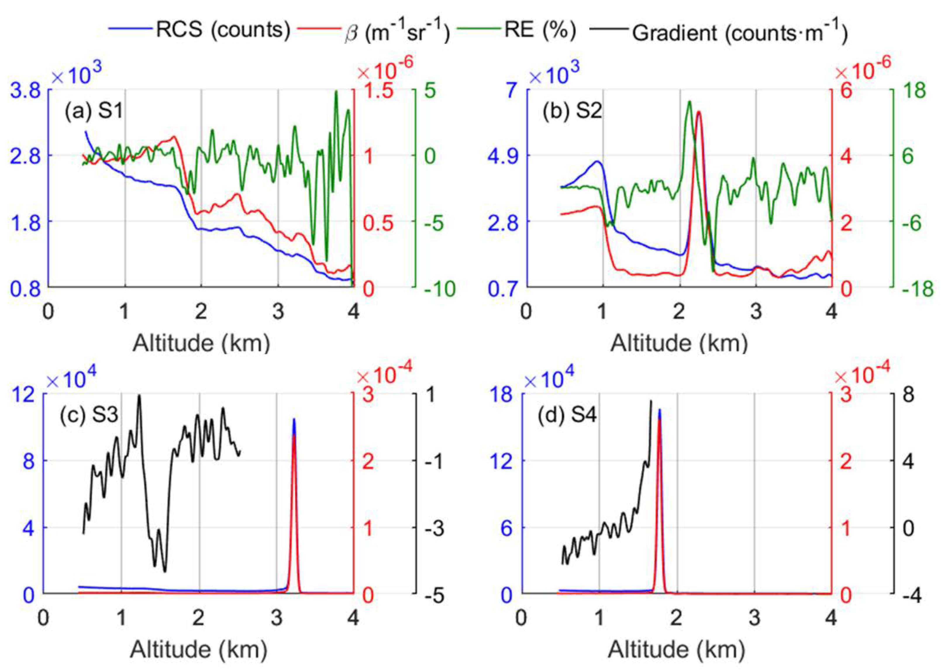
2.2. PBLH Detection Methods

The gradient method (GM) [21,35] derives the PBLH according to the change of the attenuation rate of RCS with height. This method is based on the calculated gradient of the RCS profile, and the gradient is expressed as:

$$Grad\left(R\right)=\nabla X(R)$$

(2)

The PBLH is located at the position where RCS decays fastest, namely, the height where Grad(R) gets the minimum value. The GM is simple in principle and easy to implement, and has been widely used in the inversion of boundary layer height. However, it is sensitive to noise.

The wavelet covariance transform method (WCT) [23,36] is a method to find the step change of signal. The WCT is defined as:

$$W(a,b)=\frac{1}{a}{\displaystyle {\int }_{R_b}^{R_t}X(R)h(\frac{R-b}{a})}dR$$

(3)

with the Haar wavelet function

$$h(\frac{R-b}{a})=\{\begin{array}{ll}-1,& b-\frac{a}{2}\le R\le b\\ 1,& b\le R\le b+\frac{a}{2}\\ 0,& others\end{array},$$

(4)

where R_b and R_t are the lower and upper limits of the RCS, respectively. The parameter b is the translation of the wavelet and a is the wavelet dilation ($a=n\Delta R$, $\Delta R$ is the vertical resolution of the lidar data). The optimum value for a is equal to the depth of the transition zone, which should be tested before being used. In fact, the WCT method calculates the similarity of Haar wavelet function and RCS. The larger the WCT function is, the more similar RCS and wavelet function are, that is, the more obvious the step change is. Therefore, the height of the maximum value obtained by WCT function is the PBLH.

The curve fitting method (CFM) [22,37] determines the PBLH from lidar data through fitting an idealized backscatter profile to the lidar observed backscatter profile by minimizing the difference between the two profiles. The ideal profile is expressed as:

$$D(R)=\frac{D_m+D_u}{2}-\frac{D_m-D_u}{2}erf\left(\frac{R-R_m}{s}\right)$$

(5)

with the error function

$$erf(a)=\frac{2}{\sqrt{\pi }}{\displaystyle {\int }_0^a\exp \left(-y^2\right)}dy,$$

(6)

where D_m is the mean RCS values for the maxed layer, D_u is the average RCS values for the free troposphere, R_m is the maxed layer height and s is related to the entrainment zone thickness. When the idealized profile and RCS profile are most consistent, the corresponding height parameter is the PBLH.

The standard deviation method (STD) [24,38] extracts the PBLH by the dispersion of RCS in a certain height range. The STD is expressed as:

$$STD(R)={\left\{\frac{1}{N}{\displaystyle \sum _{i=1}^N{\left[X_i(R)-\overline{X(R)}\right]}^2}\right\}}^{1/2},$$

(7)

where N corresponds to the number of profiles. The PBLH is defined as the height where the maximum STD of RCS occurs.

2.3. Lidar Data and Sounding Data

Table 1. Descriptions of the three sites with lidar date and fine-resolution sounding profiles.

Sites	Location	Altitude (m)	Date	Launch Time of Radiosonde (LT)
SGP	36.6°N, 97.3°W	315	Aug, 2017	05:30, 11:30, 17:30 and 23:30
Seoul, Korea	37.5°N, 126.9°E	135	Feb, 2018	03:00, 09:00, 15:00 and 21:00
Madison, WI	43.1°N, 89.4°W	210	Feb and May, 2017 Mar and Apr, 2020	07:00 and 19:00

illustrates the sites specifications of the three field campaigns from which lidar data and fine-resolution sounding data were collected for use in this study. The Vaisala RS92 radiosondes are launched four times a day at the Southern Great Plains, USA (SGP) site and the Seoul site, and twice a day at the Madison site [39]. PBLH is related to the vertical gradient characteristics of atmospheric thermodynamic structure. Theoretically, the temperature will increase sharply near the top of the PBL. The PBLH determined by temperature-gradient is used to evaluate the height estimated from four lidar methods [7]. The PBL structure is divided into three types: stable boundary layer, convective boundary layer and neutral residual layer, before using the vertical temperature profile from radiosonde to determine the PBLH [40,41]. For the convective boundary layer and the neutral residual layer, PBLH is the height where the temperature gradient is greater than 1 for the first time, while for stable boundary layer, PBLH is the height of inversion top where the temperature gradient is less than 6.5 for the first time, due to strong inversion for stable stratification [42]. The lidar data used in this study is the combined channel signal in high-spectral-resolution lidar (HSRL) of the University of Wisconsin [43], which is equivalent to Mie-scattering signal [44,45]. The HSRL emits laser pulses with a wavelength of 532 nm. Due to the incomplete overlap between the laser radar beam and the receiving optical axis, a blind area exists, which limits the application of the backscatter lidar near surface. The blind zone is 0.5 km and, therefore, RCS within 0.5 km above ground level (AGL) is removed. The region of incomplete overlap is corrected [43,46].

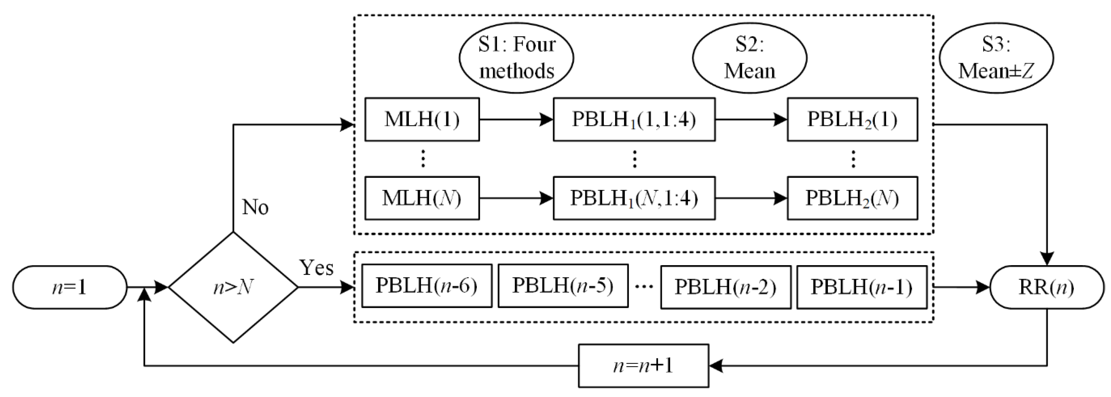
3. A Methodology to Improve the Accuracy of PBLH Determination

To eliminate the disturbance of multi-layer conditions (elevated aerosols and clouds) and improve the accuracy of PBLH determination, the maximum limited height initialization and range restriction (MLHI-RR) method is proposed. This method is comprised of two steps: initializing the maximum limited height (MLH) and setting height range restriction (RR). Figure 2 shows a simple flowchart of initializing the MLH, where X_i denotes one RCS profile, β_i is the backscatter coefficient profile of corresponding RCS and i is the variable of iteration which increases by 1 for each loop. This flowchart consists of four major steps:

First of all, it is of great significance to identify the elevated aerosols or clouds accurately on the signal profile. In the single layer case, the backscatter signal decreases linearly with height within the PBL. However, when an aloft layer of aerosol or cloud in general is presented, a strong positive gradient can be observed on the single profile. The backscatter coefficient represents the scattering ability of aerosol to light wave, and the positive gradient changes more obviously on the backscatter coefficient profile [47]. Based on this characteristic, separated aerosol layers can be identified by looking for a strong positive gradient on the backscatter coefficient profile. The analyses based on many aloft aerosol layer cases prove that the relative increase ($RE=\left(\beta (z+\Delta z)-\beta \left(z\right)\right)/\beta \left(z\right)$) in the backscatter coefficient profile of at least 10% is required, which is applicable over 532 nm lidar. Therefore, in this study, the empirical threshold of aloft aerosol layers is set when the RE is greater than 10%. Sometimes, very thin clouds near the surface might be interpreted as suspended aerosol layers, which do not have a major impact on the algorithm. Unlike aerosol, the backscatter coefficient of cloud is much larger [48], and can easily be identified by setting a threshold. We define the cloud base in much the same way as other previous studies [49,50,51]. A statistical result relying on many cloudy cases proves that the threshold of backscatter coefficient is more than $2\times {10}^{-4}$ m⁻¹sr⁻¹, which can accurately identify the cloud layer. Due to the deviation of the backscattering coefficient, it is impossible to completely use these two thresholds in any 532 nm lidar. However, these two thresholds are related to the wavelength and aerosol of lidar, but not to the signal value. Therefore, they can be used as reference values for other stations with 532 nm lidar.

While only suspended aerosol layer above the PBL are taken into account, the cloud either above or within the PBL are considered influential. If a cloud layer is detected, it is necessary to classify whether the cloud is above the PBL or within the PBL. When the cloud is above the PBL, the signal below the cloud base still shows a sharp decrease at the PBLH. Instead, when the cloud is within the PBL, the aerosol concentration below the cloud should be vertically uniform, due to convective mixing, and no change of gradient could be found. Based on many cases of clouds outside the PBL, it was found that, for the Mie-scattering signal from University of Wisconsin lidar, if clouds are visually located above the top of the PBL, a strong signal gradient of at least less than −4 generally exists below the cloud base [28] Hence, in this study, if at least one signal gradient below the lowest cloud base is less than the threshold of −4, the cloud is classified as higher than the PBL. In contrast, the cloud is thought to be within the PBL. The threshold in this work is set based on statistical analysis, which means biases and errors are included. The threshold of −4 may not be representative, but the principle for threshold selection can be applied to other observation sites.

The third step is to determine the MLH of each single profile. If the lowest cloud is separated from the PBL, the base of this cloud layer is considered to be the MLH. In contrast, if the lowest cloud is within the PBL, the PBLH cannot be retrieved, and the MLH is marked as 0. When aloft aerosol layer is identified, the base of aloft layer is considered to be the MLH. As for aerosols presented only within the PBL, in the absence of clouds or aloft aerosol layers, that is, a single aerosol layer, 4 km is deemed to be the MLH, because the PBLH is generally less than 4 km [52].

Finally, it is judged whether the MLH of the initial backscatter signal profiles is effective. In this study, the temporal resolution of the signal is 30 s and the PBL is considered rather constant within 3 min, so that the MLH of the first six single profiles is calculated (N = 6 in Figure 2). Furthermore, N can choose different values on the basis of the characteristics of the PBLH at different locations. However, it must be ensured that the PBLH does not change much in the selected period. If there is 0 among these six MLH, it means that there is cloud within PBL. In this case, PBLH cannot be determined and initialization of MLH is not successful. The algorithm is set to calculate the MLH of the next signal profile, until six consecutive effective MLH is obtained.

For clarity, Figure 3 shows four concrete examples of the major steps for initializing the MLH. These are the RCS (blue line), the backscatter coefficient of atmosphere (red line), the relative increase (RE) in backscatter coefficient (green line) and the gradient of RCS with the lowest cloud base limiter (black line) on four typical situations. Figure 3a plots an example in the single aerosol layer situation at 17:30 local time (LT), 21 August 2017 over the SGP site. Under this condition, the RCS decreases with height, as the backscatter coefficient is less than $2\times {10}^{-4}$ m⁻¹sr⁻¹ and RE is less than 10%. In such situations, the MLH is 4 km AGL. In Figure 3b, observed at 05:50 LT, 20 February 2018 over the Seoul site, an obvious aerosol layer can be seen with the peak value of RCS appearing at 2.5 km. The backscatter coefficient is smaller than $2\times {10}^{-4}$ m⁻¹sr⁻¹, but RE exceeds 10%, which indicates that the aerosol layer at approximately 2.5 km is the lofted aerosol layer. In Figure 3c, a sharp increase at approximately 3.1 km AGL and a sudden decrease at 3.4 km AGL are observed in the RCS at 17:30 LT, 21 August 2017 over the SGP site. The backscatter coefficient is much larger than $2\times {10}^{-4}$ m⁻¹sr⁻¹ and the gradient of RCS below the cloud base less than −4 occur, which proves that the cloud is outside the PBL, and that the heights of the cloud base are regarded as the MLH. Figure 3d also shows the cloud layer at 11:30 LT, 29 August 2018 over the SGP site, which is similar to that in Figure 3c. The difference is that the signal is continuous and there is no strong negative signal gradient less than −4 below the cloud base, which demonstrates that the cloud is in the PBL. In such a situation, the MLH is defined as 0.

After successfully initializing the MLH, RR also needs to be determined precisely. The method of determining RR follows the idea of averaging twice and using the moving window algorithm to reduce the error. There are two aspects about averaging twice: averaging the PBLH recognized by four lidar methods, and the PBLH of two adjacent signal profiles. Regarding the moving window algorithm, it can be defined as

$$RR(n)=\{\begin{array}{ll}\frac{{\displaystyle \sum _{i=0}^{i=N}PBL{H}_2(i)}}{N}\pm Z,& n\le N\\ \frac{{\displaystyle \sum _{i=n-N}^{i=n-1}PBLH(i)}}{N}\pm Z,& n>N\end{array}$$

(8)

where n is the nth signal profile and Z is the recognition range. The PBLH of the front and rear signal profiles do not change much in 30 s [53], so the recognition range is set as Z = 0.3 km in this study, which ensures that the PBLH is within the RR. Of course, there is no particularly strict requirement on the recognition range, and it can be adjusted appropriately, according to the PBLH change. According to Equation (8), there are two circumstances to determine RR: one is used to determine RR of the first six signal profiles, and the other is used to determine RR of the nth (n > 6) signal profile. The flowchart of determining RR is shown in Figure 4, which consists of three steps. The first step is that four lidar methods are used to identify the PBLH of first six signal profiles below the MLH, each of which is denoted as four PBLH₁. In the second step, after removing the outliers, the average of the effective PBLH₁ is denoted as PBLH₂. The last step is to take the range of Z both higher and lower than the average the six PBLH₂, which is taken as RR of the first six profiles. For the nth (n > 6) signal profile, the RR(n) is obtained using the PBLH of the first N profiles by the moving window algorithm. The final PBLH is obtained by lidar method in the range of RR.

4. Results and Discussion

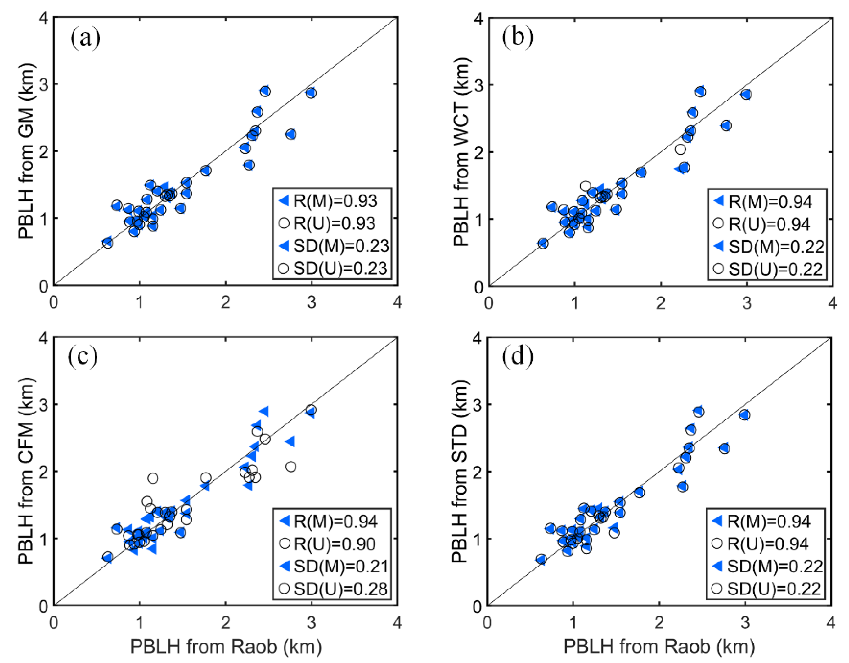
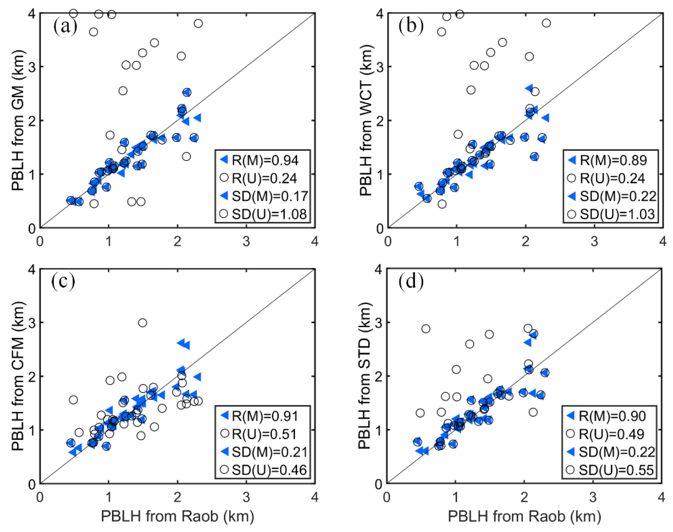
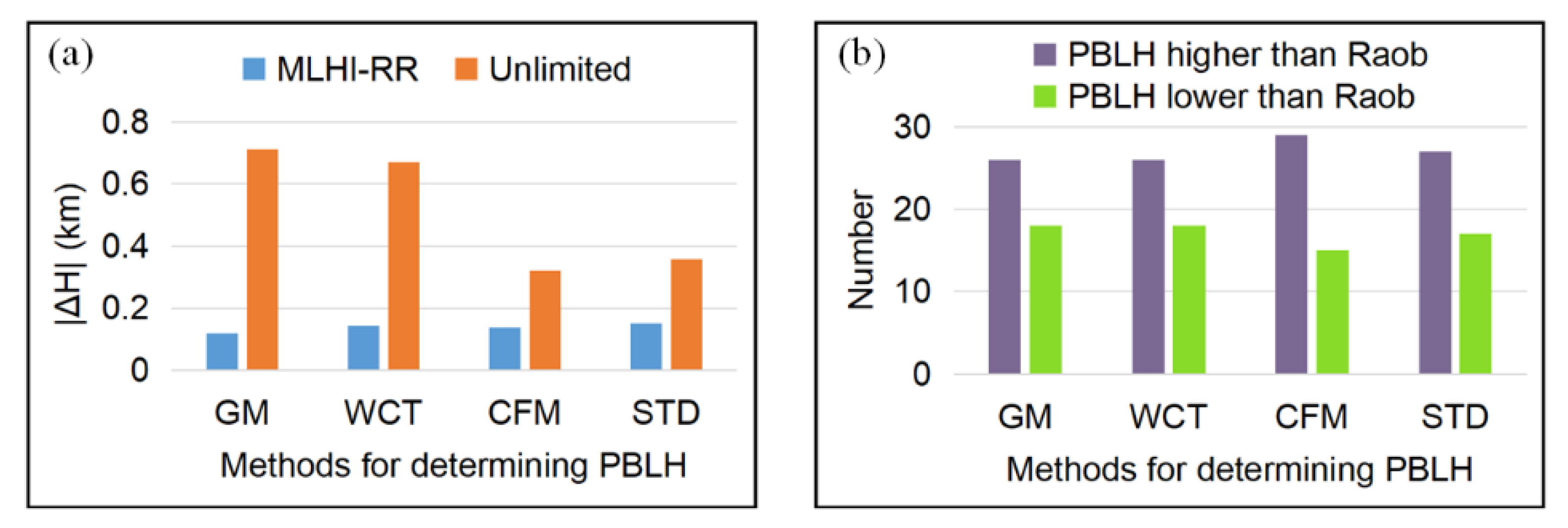
4.1. Comparisons between Lidar and Radiosonde Measurements of PBLH

The radiosonde could provide accurate thermodynamic profiles, such as temperature, for the troposphere [39,52]. The PBLH determined from radiosonde-derived profiles is frequently used to evaluate the PBLH retrieved from other measurements [53,54]. This study also evaluates the accuracy of the retrieved PBLH from lidar measurements by comparison with the PBLH from radiosonde. PBLH determined by four lidar methods is compared with that determined by the temperature-gradient method, as shown in Figure 4, Figure 5, Figure 6 and Figure 7. At 11:30 LT on 30 August 2017 at the SGP site (single aerosol layer), the PBLH determined from the temperature-gradient is 1.5225 km (Figure 5a), which is slightly lower than the height retrieved by the lidar methods. At 17:30 LT on 23 August 2017, a suspended aerosol layer above 2 km is observed (Figure 5b). Without restriction, the CFM captures the upper edge of the elevated aerosol layer, and the STD identifies the base of the aloft aerosol layer as PBLH. With initialized MLH (the lofted aerosol layer base) and setting RR, the PBLH determined from four lidar methods are between 1.5 and 1.55 km, which are closer to the PBLH determined by temperature-gradient. By setting the base of lifted aerosol layer as the upper limit and choosing reasonable range of RR, the PBLH is identified more accurately.

In total, the determined PBLH for 32 single-layer cases and 44 multi-layer cases from three sites (showed in Table 1 in Section 2.3) are compared and analyzed. The number of cases was limited, due to the lack of lidar and radiosonde data during the period, as well as the removal of some data with observed errors. As shown in Figure 6, in single aerosol layer cases, the PBLH determined by lidar measurement (vertical coordinate) and radiosonde (horizontal coordinate) are compared and found to be highly consistent. The PBLHs retrieved by four lidar methods have a correlation coefficient above 0.9 with that determined by the radiosonde. The correlation coefficients and standard deviations of GM, WCT and STD are the same with MLHI-RR (blue triangles) and without it (black circles), while the PBLH determined by CFM with MLHI-RR is slightly more accurate. The results illustrate that the lidar can accurately identify the PBLH for the case of a single aerosol layer.

While the four lidar methods have been proved to be suitable for PBLH inversion for single-layer cases, the results for multi-layer cases are very different (Figure 7). Without any limitation (black circles), the heights determined from four lidar methods are, in general, much higher than those from the temperature-gradient. The errors of the four lidar methods are notable, with low correlation coefficients with the temperature-gradient method, which is 0.24 for GM and WCT, 0.51 for CFM and 0.49 for STD. The standard deviations of the four lidar methods are large. In particular, the standard deviations of GM and WCT exceed one. The deviation between the lidar and radiosonde measurements of PBLH is mainly caused by the presence of aloft aerosol layers or clouds. There, multi-layer situations have severely affected the lidar detection of PBLH. However, after setting MLHI-RR (blue triangles), the height determined by four lidar methods showed better concordance with those by temperature-gradient, with a good correlation coefficient of about 0.9 and a low standard deviation about 0.2. For multi-layer situations, the GM performs best with MLHI-RR. The great improvement of correlation coefficient demonstrates that the influence of multi-layer situations is eliminated by using MLHI-RR.

The statistic of PBLH derived from four lidar methods with MLHI-RR and without limiter in the multi-layer conditions is compared in Figure 8a, where |ΔH| is the difference of PBLH between lidar method and radiosonde. Without any limiter, the PBLH inverted by four lidar methods has a great deviation with the altitude differences all of which are higher than 0.3 km, especially for GM (0.711 km) and WCT (0.670 km). With MLHI-RR, the altitude differences are all less than 0.2 km. Nonetheless, our comparison reaches a conclusion similar to Hennemuth and Lammert [54], which found that the PBLH based on radiosonde and lidar data deviates between ±0.2 km. The number of cases that the PBLH determined by lidar method is higher or lower than that measured by radiosonde, as summarized in Figure 8b. The PBLH from lidar tends to be somewhat higher than that from radiosonde, mainly because the lidar detects the immediate top of the inversion layer, while the temperature-gradient determines the PBLH at about the middle to the top of the inversion layer.

In general, the above comparison results show that the relatively reliable PBLH can be determined from lidar data in single aerosol layer situation. However, lofted aerosol layers or clouds will seriously interfere with the measurement of PBLH by lidar. Initializing the MLH and setting the RR can improve the accuracy of identifying PBLH in the case of complexity.

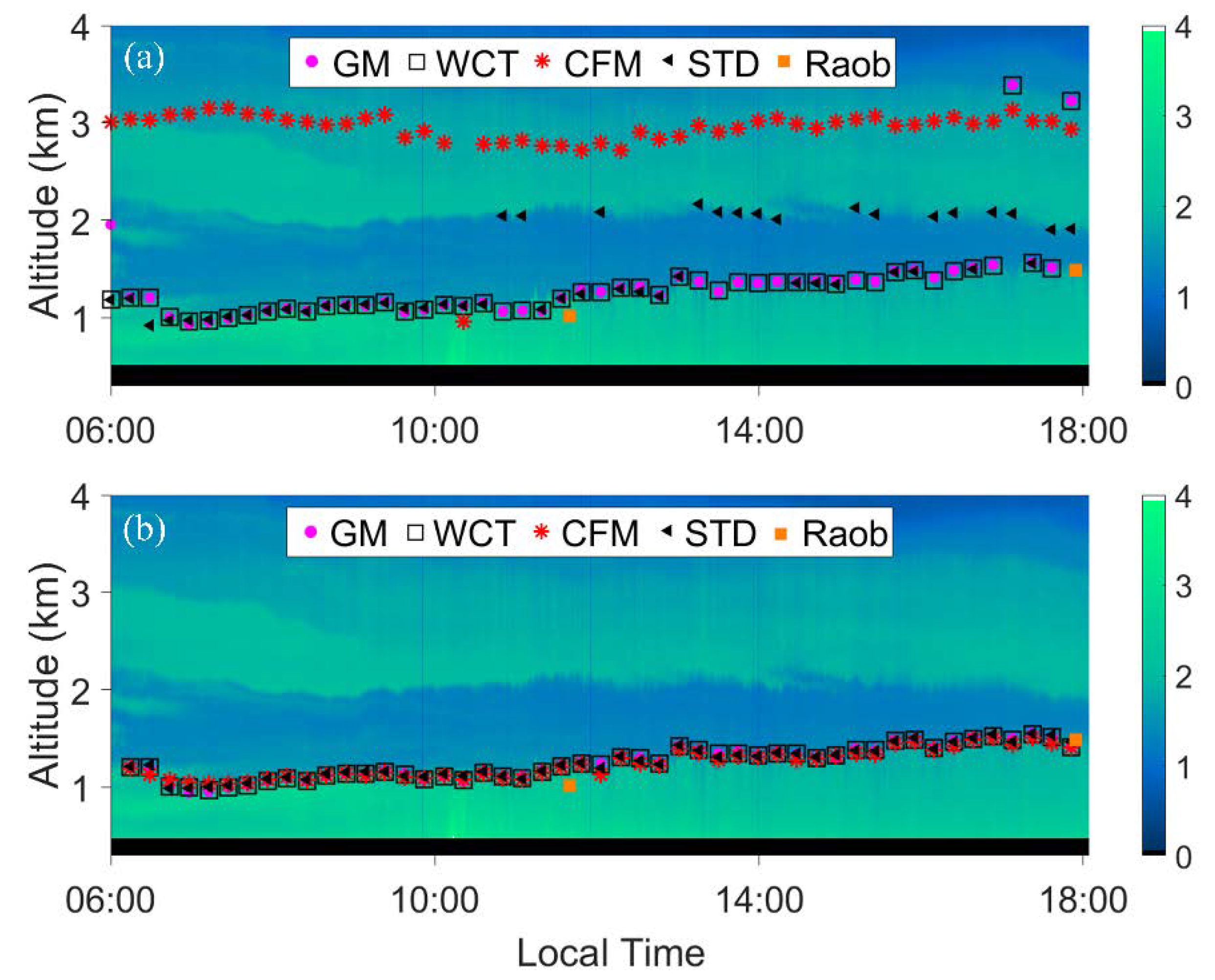
4.2. Continuous Variations in PBLH

This section presents the continuous variations in PBLH to demonstrate the proposed technique, and further test its ability for improving PBLH determination in the presence of elevated aerosols and clouds. Four measurement cases studies at the SGP site under different aerosol and meteorological conditions are discussed. The evolution of the PBLH in distinct double aerosol layer conditions is discussed first (23 August 2017). Next, a case with weak lofted aerosol layer observed on 19 August 2017 is presented. In the third case (25 August 2017), clouds complicated the PBL top detection. The elevated aerosols and clouds appear simultaneously in the fourth case (12 August 2017). As mentioned above, the temporal resolution of RCS is 30 s and the PBLH is calculated at a time interval of 30 s correspondingly. Only the time period PBLH above the lidar blind zone is studied.

The normalized RCS of the first case is as shown in Figure 9. The evolution of the double layer aerosol has been observed during 06:00–18:00 LT on 23 August 2017. The height of the near-surface aerosol layer in this period is about 1 km, and there is a distinct lofted aerosol layer between 2 km and 4 km AGL. For PBLH retrieval, without MLHI-RR, the CFM captures the height close to the upper edge of the elevated aerosol layer, the STD sometimes distinguishes the base of the aloft aerosol layer as PBLH, and the GM and WCT occasionally make mistakes as well (Figure 9a). The CFM has problems on account of no clear signal step function during this period. After initializing MLH and setting RR (Figure 9b), compared with the PBLH determined by temperature-gradient method (orange squares), the PBLH is then successfully determined by four lidar methods. The GM and WCT methods work best under these complex conditions of aerosol layers. The outcome of the comparison results state clearly that the new technology can eliminate the effect of lofted aerosol layers. Furthermore, the PBLH identified by the four lidar methods is more consistent using the MLHI-RR technique.

In a clear day and small wind, the misty elevated aerosols frequently appear, with the result being that the lidar measurements of PBLH may be seriously influenced. Figure 10 shows the PBL evolution in terms of normalized RCS observed with lidar on 19 August 2017. From 10:00–13:00 LT, misty elevated aerosols above the PBL complicate the retrieval of the PBLH. It is clear to see the top of the lifted aerosol layer during 10:00–11:00 LT. Gradually, the lifted aerosol layer becomes unapparent. The results regarding the retrieval of PBL top with the four lidar methods are shown in Figure 10. Without any limitation, it can be seen in Figure 10a that none of the four lidar methods can successfully identify true PBLH over time. The CFM captures the altitude higher than the PBLH affected by the elevated aerosols. Moreover, the GM, WCT and STD are easily affected by the elevated aerosols when the signal negative gradient at the lofted layer top is stronger than that at the top of the near surface aerosol layer. After using the MLHI-RR, four lidar methods are able to detect the PBLH accurately (Figure 9b). The comparison results prove that the new technology put forward in this paper can eliminate the influence of the misty elevated aerosols.

In contrast, on 25 August 2017 between 11:00 and 14:00 LT, clouds formed near the top of the PBL, which is presented as a blank region in Figure 11. As a result of the thick cloud layers, the temperature provided by the radiosonde is of poor quality, so the PBLH retrieved from temperature-gradient method is not considered. The signal above the clouds is completely attenuated. The potential of the technique proposed in this study for determining cloud layers and eliminating their effect is discussed in this case. From 11:00 to 11:20 LT, there was a distinct surface aerosol layer and a strong signal negative gradient below the cloud base, indicating that the cloud base was higher than the PBL. As shown in Figure 11a, the cloud influences the PBLH determination as four lidar methods capture the edge of the cloud without restriction. While the GM, WCT and STD are capable of accurately capturing the PBLH with the MLHI-RR when the cloud is outside the PBL (Figure 11b), the CFM obtained the upper edge of the cloud or the top of residual layer. The CFM could not accurately determine the actual PBLH because the information of clean area is unable to be obtained under the interference of clouds [55]. As for the cloud within the PBL, the upper edge of the clouds is regarded as the PBLH. However, it is difficult to determine PBLH accurately based on lidar data for these cloud layers, because defining the cloud upper edge as the PBLH is not appropriate in such a situation.

Figure 12 shows another case, 25–26 August 2017, which is a cloudy day with lofted aerosol layer between 02:00 and 06:00 LT. There is a thin cloud layer (blank region) above 2 km AGL from 21:30 to 04:30. The PBLH determined by temperature-gradient method at 23:30 LT and 05:30 LT are 0.7950 km and 0.7875 km. Without any limitation, four lidar methods are all wrong when capturing the edge of the cloud or the elevated aerosol layer (Figure 12a). As shown in Figure 12b, the addition of the MLHI-RR improves the results, causing the resulting PBLH of the GM, WCT and STD to conform the more typical evolution of the PBLH, and to be closer to the PBLH estimated by the temperature-gradient method. Although there are clouds and elevated aerosols simultaneously, the technology proposed in this paper can effectively eliminate the effect. However, the CFM performs poorly, as it regards the cloudy boundary as PBLH. Combined with the results and analysis in Figure 11, it can be seen that CFM is not suitable for retrieving the PBLH under the situation with cloud.

Lidar is a powerful remote sensing instrument for detecting the PBL, but the appearance of cloud and elevated aerosol layers effect the accuracy of PBLH determination. The technique proposed in the study performs well on improving lidar measurements of PBLH in the appearance of cloud and elevated aerosol layers. However, the limitation of the technique is inevitable. First of all, the selection of the threshold to determine whether the cloud is outside the PBL depends on statistics and experience, and this threshold is related to the intensity of the lidar signal, which needs to be adjusted according to the amplitude of the instrument signal. However, the principle for threshold determination is clear and reasonable, and it can be applied to other observation sites. Secondly, the CFM is not suitable for determining the PBLH with this technique in the cloudy situation for the information of the clean area is unable to be obtained under the interference of clouds (especially low altitude clouds). However, the other three lidar methods determine PBLH accurately.

5. Conclusions

In this study, a new technique named the MLHI-RR was proposed, to improve the accuracy of PBLH determined by lidar under multi-layer conditions. There are two aspects (initializing MLH and setting RR) in terms of improving the applicability of the algorithm. It is first and foremost to identify the elevated aerosols and clouds by looking for relative increases in the lidar profiles of backscatter coefficient. Then, the cloud above the PBL or within the PBL is classified by finding a strong negative gradient on RCS smaller than an empirical threshold of −4 below the cloud base. The third step is to determine the MLH in different situations, followed by judging whether consecutive MLH is effective. Finally, an appropriate RR is acquired by taking advantage of averaging twice and the moving window algorithm.

For the evaluation of the new technique, the PBLH of 44 multi-layer cases retrieved from four lidar methods are compared with the radiosonde-based retrievals. Without restriction, the lidar-estimated heights are usually much higher than radiosonde-based PBLH, because the lidar methods often discern the lofted layer edge. When the MLHI-RR technique is applied, a good consistency (R = 0.9) was achieved between the lidar-determined PBLH and those from temperature-gradient. Four case studies with continuous variations in PBLH are also analyzed, which shows lidar methods can retrieve the true PBLH after utilizing the MLHI-RR method. That is, the technique effectively eliminated the disturbance of multi-layers on PBLH determination. Experimental results indicated the viability of this technique under multi-layer conditions which can be problematic for prior methods. What’s more, the PBLH determined by the GM is best with MLHI-RR in multi-layer situations. The CFM is not suitable for retrieving the PBLH in cloudy situations. Furthermore, the technique has not been tested on the lidar of other research institutions, the advantages of this technique will be extended to the lidar data in future studies.

References

1. Stull, R.B. An introduction to boundary layer meteorology. Atmos. Sci. Libr. 1988, 8, 89. [Google Scholar]
2. Liu, D.; Chen, S.; Cheng, C.; Barker, H.W.; Dong, C.; Ke, J.; Wang, S.; Zheng, Z. Analysis of global three-dimensional aerosol structure with spectral radiance matching. Atmos. Meas. Tech. 2019, 12, 6541–6556. [Google Scholar] [CrossRef] [Green Version]
3. Wang, X.Y.; Wang, K.C. Estimation of atmospheric mixing layer height from radiosonde. Atmos. Meas. Tech. 2014, 7, 1701–1709. [Google Scholar] [CrossRef] [Green Version]
4. D’Asaro, E.; Lee, C.; Rainville, L.; Harcourt, R.; Thomas, L. Enhanced Turbulence and Energy Dissipation at Ocean Fronts. Science 2011, 332, 318–322. [Google Scholar] [CrossRef] [Green Version]
5. Holtslag, A.A.M.; Boville, B.A. Local Versus Nonlocal Boundary-Layer Diffusion in a Global Climate Model. J. Clim. 1993, 6, 1825–1842. [Google Scholar] [CrossRef] [Green Version]
6. Basha, G.; Ratnam, M.V. Identification of atmospheric boundary layer height over a tropical station using high-resolution radiosonde refractivity profiles: Comparison with GPS radio occultation measurements. J. Geophys. Res. Atmos. 2009, 114, 11. [Google Scholar] [CrossRef]
7. Seidel, D.J.; Ao, C.O.; Li, K. Estimating climatological planetary boundary layer heights from radiosonde observations: Comparison of methods and uncertainty analysis. J. Geophys. Res. Atmos. 2010, 115, 15. [Google Scholar] [CrossRef] [Green Version]
8. Seibert, P.; Beyrich, F.; Gryning, S.E.; Joffre, S.; Rasmussen, A.; Tercier, P. Review and intercomparison of operational methods for the determination of the mixing height. Atmos. Environ. 2000, 34, 1001–1027. [Google Scholar] [CrossRef]
9. Helmis, C.G.; Sgouros, G.; Tombrou, M.; Schaefer, K.; Muenkel, C.; Bossioli, E.; Dandou, A. A Comparative Study and Evaluation of Mixing-Height Estimation Based on Sodar-RASS, Ceilometer Data and Numerical Model Simulations. Bound. Layer Meteorol. 2012, 145, 507–526. [Google Scholar] [CrossRef]
10. Bianco, L.; Wilczak, J.M. Convective boundary layer depth: Improved measurement by Doppler radar wind profiler using fuzzy logic methods. J. Atmos. Ocean. Technol. 2002, 19, 1745–1758. [Google Scholar] [CrossRef]
11. Wang, D.; Stachlewska, I.S.; Song, X.; Heese, B.; Nemuc, A. Variability of the Boundary Layer Over an Urban Continental Site Based on 10 Years of Active Remote Sensing Observations in Warsaw. Remote Sens. 2020, 12, 340. [Google Scholar] [CrossRef] [Green Version]
12. Wiegner, M.; Madonna, F.; Binietoglou, I.; Forkel, R.; Gasteiger, J.; Geiß, A.; Pappalardo, G.; Schäfer, K.; Thomas, W. What is the benefit of ceilometers for aerosol remote sensing? An answer from EARLINET. Atmos. Meas. Tech. 2014, 7, 1979–1997. [Google Scholar] [CrossRef] [Green Version]
13. Haeffelin, M.; Angelini, F.; Morille, Y.; Martucci, G.; Frey, S.; Gobbi, G.P.; Lolli, S.; O’Dowd, C.D.; Sauvage, L.; Xueref-Remy, I.; et al. Evaluation of Mixing-Height Retrievals from Automatic Profiling Lidars and Ceilometers in View of Future Integrated Networks in Europe. Bound. Layer Meteorol. 2012, 143, 49–75. [Google Scholar] [CrossRef]
14. Kotthaus, S.; O’Connor, E.; Muenkel, C.; Charlton-Perez, C.; Haeffelin, M.; Gabey, A.M.; Grimmond, C.S.B. Recommendations for processing atmospheric attenuated backscatter profiles from Vaisala CL31 ceilometers. Atmos. Meas. Tech. 2016, 9, 3769–3791. [Google Scholar] [CrossRef] [Green Version]
15. Tang, G.; Zhang, J.; Zhu, X.; Song, T.; Muenkel, C.; Hu, B.; Schaefer, K.; Liu, Z.; Zhang, J.; Wang, L.; et al. Mixing layer height and its implications for air pollution over Beijing, China. Atmos. Chem. Phys. 2016, 16, 2459–2475. [Google Scholar] [CrossRef] [Green Version]
16. McGrath-Spangler, E.L.; Denning, A.S. Estimates of North American summertime planetary boundary layer depths derived from space-borne lidar. J. Geophys. Res. Atmos. 2012, 117, D15101. [Google Scholar] [CrossRef] [Green Version]
17. Moreira, G.D.A.; Guerrero-Rascado, J.L.; Bravo-Aranda, J.A.; Benavent-Oltra, J.A.; Ortiz-Amezcua, P.; Róman, R.; Bedoya-Velásquez, A.E.; Landulfo, E.; Alados-Arboledas, L. Study of the planetary boundary layer by microwave radiometer, elastic lidar and Doppler lidar estimations in Southern Iberian Peninsula. Atmos. Res. 2018, 213, 185–195. [Google Scholar] [CrossRef] [Green Version]
18. Milroy, C.; Martucci, G.; Lolli, S.; Loaec, S.; Sauvage, L.; Xueref-Remy, I.; Lavrič, J.V.; Ciais, P.; Feist, D.G.; Biavati, G.; et al. An Assessment of Pseudo-Operational Ground-Based Light Detection and Ranging Sensors to Determine the Boundary-Layer Structure in the Coastal Atmosphere. Adv. Meteorol. 2012, 2012, 929080. [Google Scholar] [CrossRef] [Green Version]
19. Emeis, S.; Schaefer, K.; Muenkel, C. Surface-based remote sensing of the mixing-layer height—A review. Meteorol. Z. 2008, 17, 621–630. [Google Scholar] [CrossRef] [PubMed]
20. Tang, P.; Liu, D.; Xu, P.; Zhou, Y.; Bai, J.; Liu, C.; Wang, K.; Yang, Y.; Shen, Y.; Luo, J.; et al. Detection of atmospheric boundary layer height in the plum rain season over Hangzhou area with three-dimensional scanning polarized lidar. In Proceedings of the Optoelectronic Devices and Integration VI, Beijing, China, 12–14 October 2016. [Google Scholar]
21. Flamant, C.; Pelon, J.; Flamant, P.H.; Durand, P. Lidar determination of the entrainment zone thickness at the top of the unstable marine atmospheric boundary layer. Bound. Layer Meteorol. 1997, 83, 247–284. [Google Scholar] [CrossRef]
22. Steyn, D.G.; Baldi, M.; Hoff, R.M. The detection of mixed layer depth and entrainment zone thickness from lidar backscatter profiles. J. Atmos. Ocean. Technol. 1999, 16, 953–959. [Google Scholar] [CrossRef]
23. Compton, J.C.; Delgado, R.; Berkoff, T.A.; Hoff, R.M. Determination of Planetary Boundary Layer Height on Short Spatial and Temporal Scales: A Demonstration of the Covariance Wavelet Transform in Ground-Based Wind Profiler and Lidar Measurements. J. Atmos. Ocean. Technol. 2013, 30, 1566–1575. [Google Scholar] [CrossRef]
24. Menut, L.; Flamant, C.; Pelon, J.; Flamant, P.H. Urban boundary-layer height determination from lidar measurements over the Paris area. Appl. Opt. 1999, 38, 945–954. [Google Scholar] [CrossRef]
25. Angevine, W.M.; White, A.B.; Avery, S.K. Boundary-layer depth and entrainment zone characterization with a boundary-layer profiler. Bound. Layer Meteorol. 1994, 68, 375–385. [Google Scholar] [CrossRef]
26. Toledo, D.; Cordoba-Jabonero, C.; Antonio Adame, J.; De La Morena, B.; Gil-Ojeda, M. Estimation of the atmospheric boundary layer height during different atmospheric conditions: A comparison on reliability of several methods applied to lidar measurements. Int. J. Remote Sens. 2017, 38, 3203–3218. [Google Scholar] [CrossRef]
27. Chen, S.; Cheng, C.; Zhang, X.; Su, L.; Tong, B.; Dong, C.; Wang, F.; Chen, B.; Chen, W.; Liu, D. Construction of Nighttime Cloud Layer Height and Classification of Cloud Types. Remote Sens. 2020, 12, 668. [Google Scholar] [CrossRef] [Green Version]
28. Dang, R.; Yang, Y.; Li, H.; Hu, X.-M.; Wang, Z.; Huang, Z.; Zhou, T.; Zhang, T. Atmosphere Boundary Layer Height (ABLH) Determination under Multiple-Layer Conditions Using Micro-Pulse Lidar. Remote Sens. 2019, 11, 263. [Google Scholar] [CrossRef] [Green Version]
29. Wang, C.; Shi, H.; Jin, L.; Chen, H.; Wen, H. Measuring boundary-layer height under clear and cloudy conditions using three instruments. Particuology 2016, 28, 15–21. [Google Scholar] [CrossRef]
30. Liu, B.; Zhong, Z.; Zhou, J. Development of a Mie scattering lidar system for measuring whole tropospheric aerosols. J. Opt. A Pure Appl. Opt. 2007, 9, 828–832. [Google Scholar] [CrossRef]
31. Liu, D.; Yang, Y.; Cheng, Z.; Huang, H.; Zhang, B.; Ling, T.; Shen, Y. Retrieval and analysis of a polarized high-spectral-resolution lidar for profiling aerosol optical properties. Opt. Express 2013, 21, 13084–13093. [Google Scholar] [CrossRef] [PubMed]
32. Fernald, F.G. Analysis of atmospheric lidar observations: Some comments. Appl. Opt. 1984, 23, 652–653. [Google Scholar] [CrossRef]
33. Sasano, Y. Tropospheric aerosol extinction coefficient profiles derived from scanning lidar measurements over Tsukuba, Japan, from 1990 to 1993. Appl. Opt. 1996, 35, 4941–4952. [Google Scholar] [CrossRef] [PubMed] [Green Version]
34. Mao, F.; Gong, W.; Li, C. Anti-noise algorithm of lidar data retrieval by combining the ensemble Kalman filter and the Fernald method. Opt. Express 2013, 21, 8286–8297. [Google Scholar] [CrossRef] [PubMed]
35. Tsaknakis, G.; Papayannis, A.; Kokkalis, P.; Amiridis, V.; Kambezidis, H.D.; Mamouri, R.E.; Georgoussis, G.; Avdikos, G. Inter-comparison of lidar and ceilometer retrievals for aerosol and Planetary Boundary Layer profiling over Athens, Greece. Atmos. Meas. Tech. 2011, 4, 1261–1273. [Google Scholar] [CrossRef] [Green Version]
36. Lewis, J.R.; Welton, E.J.; Molod, A.M.; Joseph, E. Improved boundary layer depth retrievals from MPLNET. J. Geophys. Res. Atmos. 2013, 118, 9870–9879. [Google Scholar] [CrossRef]
37. Mok, T.M.; Rudowicz, C.Z. A lidar study of the atmospheric entrainment zone and mixed layer over Hong Kong. Atmos. Res. 2004, 69, 147–163. [Google Scholar] [CrossRef]
38. Lammert, A.; Boesenberg, J. Determination of the convective boundary-layer height with laser remote sensing. Bound. Layer Meteorol. 2006, 119, 159–170. [Google Scholar] [CrossRef]
39. Jensen, M.P.; Holdridge, D.J.; Survo, P.; Lehtinen, R.; Baxter, S.; Toto, T.; Johnson, K.L. Comparison of Vaisala radiosondes RS41 and RS92 at the ARM Southern Great Plains site. Atmos. Meas. Tech. 2016, 9, 3115–3129. [Google Scholar] [CrossRef] [Green Version]
40. Vogelezang, D.H.P.; Holtslag, A.A.M. Evaluation and model impacts of alternative boundary-layer height formulations. Bound. Layer Meteorol. 1996, 81, 245–269. [Google Scholar] [CrossRef]
41. Zhang, Y.; Gao, Z.; Li, D.; Li, Y.; Zhang, N.; Zhao, X.; Chen, J. On the computation of planetary boundary-layer height using the bulk Richardson number method. Geosci. Model Dev. 2014, 7, 2599–2611. [Google Scholar] [CrossRef] [Green Version]
42. Liu, S.; Liang, X.-Z. Observed Diurnal Cycle Climatology of Planetary Boundary Layer Height. J. Clim. 2010, 23, 5790–5809. [Google Scholar] [CrossRef]
43. Grund, C.J.; Eloranta, E.W. University of Wisconsin High Spectral Resolution Lidar. Opt. Eng. 1991, 30, 6–12. [Google Scholar] [CrossRef]
44. Liu, D.; Hostetler, C.; Miller, I.; Cook, A.; Hair, J. System analysis of a tilted field-widened Michelson interferometer for high spectral resolution lidar. Opt. Express 2012, 20, 1406–1420. [Google Scholar] [CrossRef] [PubMed]
45. Zhang, Y.; Liu, D.; Shen, X.; Bai, J.; Liu, Q.; Cheng, Z.; Tang, P.; Yang, L. Design of iodine absorption cell for high-spectral-resolution lidar. Opt. Express 2017, 25, 15913–15926. [Google Scholar] [CrossRef] [PubMed]
46. Eloranta, E.W.; Razenkov, I.A.; Garcia, J.P.; Hedrick, J. Observations with the university of Wisconsin arctic high spectral resolution lidar. In Proceedings of the 22nd International Laser Radar Conference, Matera, Italy, 12–16 July 2004; Volume 561, pp. 305–308. [Google Scholar]
47. Liu, D.; Yang, Y.; Zhang, Y.; Cheng, Z.; Wang, Z.; Luo, J.; Su, L.; Yang, L.; Shen, Y.; Bai, J.; et al. Pattern recognition model for aerosol classification with atmospheric backscatter lidars: Principles and simulations. J. Appl. Remote Sens. 2015, 9, 096006. [Google Scholar] [CrossRef]
48. Berthier, S.; Chazette, P.; Pelon, J.; Baum, B. Comparison of cloud statistics from spaceborne lidar systems. Atmos. Chem. Phys. 2008, 8, 6965–6977. [Google Scholar] [CrossRef] [Green Version]
49. Mao, F.; Gong, W.; Zhu, Z. Simple multiscale algorithm for layer detection with lidar. Appl. Opt. 2011, 50, 6591–6598. [Google Scholar] [CrossRef] [PubMed]
50. Wang, Z.; Sassen, K. Cloud type and macrophysical property retrieval using multiple remote sensors. J. Appl. Meteorol. 2001, 40, 1665–1682. [Google Scholar] [CrossRef]
51. Pal, S.R.; Steinbrecht, W.; Carswell, A.I. Automated method for lidar determination of cloud-base height and vertical extent. Appl. Opt. 1992, 31, 1488–1494. [Google Scholar] [CrossRef]
52. Schmid, P.; Niyogi, D. A Method for Estimating Planetary Boundary Layer Heights and Its Application over the ARM Southern Great Plains Site. J. Atmos. Ocean. Technol. 2012, 29, 316–322. [Google Scholar] [CrossRef] [Green Version]
53. Baars, H.; Ansmann, A.; Engelmann, R.; Althausen, D. Continuous monitoring of the boundary-layer top with lidar. Atmos. Chem. Phys. 2008, 8, 7281–7296. [Google Scholar] [CrossRef] [Green Version]
54. Hennemuth, B.; Lammert, A. Determination of the Atmospheric Boundary Layer Height from Radiosonde and Lidar Backscatter. Bound. Layer Meteorol. 2005, 120, 181–200. [Google Scholar] [CrossRef]
55. Dang, R.; Yang, Y.; Hu, X.-M.; Wang, Z.; Zhang, S. A Review of Techniques for Diagnosing the Atmospheric Boundary Layer Height (ABLH) Using Aerosol Lidar Data. Remote Sens. 2019, 11, 1590. [Google Scholar] [CrossRef] [Green Version]
Figure 1. The sketch of Mie-scattering lidar system.
Remotesensing 12 02272 g001
Figure 2. Major steps for initializing the maximum limited height (MLH) under elevated aerosols and clouds situations.
Remotesensing 12 02272 g002
Figure 3. Vertical distributions of range-corrected signal (RCS) (blue line), backscatter coefficient (β) (red line), relative increase in backscatter coefficient (green line) and gradient of RCS with the lowest cloud base limiter (black line) on four typical situations: (a) single aerosol layer, observed at 17:30 LT, 21 August 2017 over the Southern Great Plains (SGP) site; (b) lofted aerosol layer, observed at 05:50 LT, 20 February 2018 over the Seoul site; (c) cloud layer outside the planetary boundary layer (PBL) is observed at 11:50 LT, 5 August 2018 over the SGP site and (d) cloud layer within the PBL is observed at 11:30 LT, 29 August 2018 over the SGP site.
Remotesensing 12 02272 g003
Figure 4. Schematic diagram of determining the range restriction (RR).
Remotesensing 12 02272 g004
Figure 5. Vertical profiles of lidar RCS (blue line) and temperature (red line) at the SGP site. The profiles were observed (a) at 11:30 LT on 30 August 2017 (single aerosol layer) and (b) at 17:30 LT on 23 August 2017 (double aerosol layers), respectively. The planetary boundary layer height (PBLH) determined using four lidar methods are marked in different sharps. The red dashed horizontal line shows the PBLH determined by temperature-gradient. h(T) is the PBLH determined by temperature-gradient. M stands for maximum limited height initialization and range restriction (MLHI-RR) and U stands for unlimited in Figure 4b.
Remotesensing 12 02272 g005
Figure 6. Comparison between radiosonde-determined (horizontal coordinate) and lidar measurement (vertical coordinate) of PBLH by (a) the gradient method (GM), (b) the wavelet covariance transform method (WCT), (c) the curve fitting method (CFM) and (d) the standard deviation method (STD) on 32 cases in single aerosol layer situations. The blue triangles and the black circles represent the comparison results with MLHI-RR and without limiter, respectively. The correlation coefficients are represented by R and standard deviations are represented by SD. The black solid line is the 1:1 line. M stands for MLHI-RR and U stands for unlimited.
Remotesensing 12 02272 g006
Figure 7. Similar to Figure 6, but in multi-layer conditions.
Remotesensing 12 02272 g007
Figure 8. In the multi-layer conditions, comparing (a) the divergence of the PBLH derived from radiosonde and four lidar methods with MLHI-RR and without limiter; (b) the relative height of PBLH from lidar with MLHI-RR and radiosonde.
Remotesensing 12 02272 g008
Figure 9. Evolution of the PBL at double layer aerosol conditions observed with backscatter lidar (range-corrected 532 nm signal, 30 s, 7.5 m resolution) on 23 August 2017. (a) PBLH determined directly from four lidar methods without restriction. (b) PBLH determined from the four lidar methods after initializing MLH and setting RR.
Remotesensing 12 02272 g009
Figure 10. Same as Figure 9, except for the misty elevated aerosols 19 August 2017, 10:00–13:00 LT.
Remotesensing 12 02272 g010
Figure 11. Same as Figure 9, except for 25 August 2017, 11:00–14:00 LT. Clouds are above and within the PBL presented as a white region during this period.
Remotesensing 12 02272 g011
Figure 12. Same as Figure 9, except for 25–26 August 2017, 21:00–06:00 LT. Clouds are above and within the PBL presented as a white region during this period.
Remotesensing 12 02272 g012