Abstract
Retrieving information concerning the interior of the ocean using satellite remote sensing data has a major impact on studies of ocean dynamic and climate changes; however, the lack of information within the ocean limits such studies about the global ocean. In this paper, an artificial neural network, combined with satellite data and gridded Argo product, is used to estimate the ocean heat content (OHC) anomalies over four different depths down to 2000 m covering the near-global ocean, excluding the polar regions. Our method allows for the temporal hindcast of the OHC to other periods beyond the 2005–2018 training period. By applying an ensemble technique, the hindcasting uncertainty could also be estimated by using different 9-year periods for training and then calculating the standard deviation across six ensemble members. This new OHC product is called the Ocean Projection and Extension neural Network (OPEN) product. The accuracy of the product is accessed using the coefficient of determination (R2) and the relative root-mean-square error (RRMSE). The feature combinations and network architecture are optimized via a series of experiments. Overall, intercomparison with several routinely analyzed OHC products shows that the OPEN OHC has an R2 larger than 0.95 and an RRMSE of <0.20 and presents notably accurate trends and variabilities. The OPEN product can therefore provide a valuable complement for studies of global climate changes.
1. Introduction
In recent decades, with the continuous emission of greenhouse gases the imbalance in the top-of-atmosphere radiation has intensified, leading to continued global warming. This imbalance, termed the Earth’s energy imbalance (EEI, [1]), is a vital issue because it intensifies and promotes changes in the global climate system. Tracking the EEI is essential to studying and understanding the past, current, and future status of climate change [2]. Physically, the EEI is caused by the difference between the energy absorbed and that reflected by the Earth, i.e., the net thermal energy trapped inside the Earth system [3]. The EEI is small compared to the total amount of solar radiation, which makes it difficult to accurately quantify [2]. More than 93% of the EEI passes through the atmosphere into the ocean and is stored in the form of ocean heat content (OHC) changes [4,5]. This is not only due to the fact that the ocean accounts for approximately 71% of the global surface area and approximately 97% of the world’s total water volume but is also due to the large specific heat capacity of water in nature. Therefore, the ocean plays a tipping role in the global system. Historically, the global OHC has been important to the Earth’s heat balance at the multi-decadal scale [6]. Data indicate that, from 1953 to 2003, the global OHC has been increasing, therefore dominating the internal variability of the Earth’s heat over the past 50 years [7]. Consequently, OHC is the most suitable variable for detecting and tracking EEI changes [3].
The variability of internal ocean dynamics has been extensively studied via investigations of changes in the ocean subsurface variables, such as temperature, flow velocity, and OHC. Compared to other thermal variables, such as the sea surface temperature (SST) or subsurface temperature anomalies (STA), the OHC is more stable and can better represent low-frequency climate variability [8]. The global OHC can not only affect global climate changes but can also serve as an important indicator of ocean variability [9,10]. Climatic records suggest that, over the past decades, the warming rate of the ocean has continued to increase, reaching a record high in 2019 [11]. OHC is also related to changes in the El Niño phenomenon; therefore, studying changes in the OHC is crucial to understanding the climate [9,10].
Satellite remote sensing has the advantages of wide and near-real-time coverage and contains a large volume of spatial-temporal data. However, remote sensing can only observe the surface of the ocean and is less capable of directly detecting changes in the subsurface ocean. To overcome this limitation, promising methods capable of accurately estimating changes in the ocean interior have been developed [12]. At present, these methods of so-called subsurface and deeper ocean remote sensing (DORS) can generally be divided into three major categories: empirical statistics, data assimilation, and dynamic models [13]. The majority of previous researchers have used different surface remote sensing data to estimate ocean subsurface heat information via these three methods using deep-sea remote sensing [12,14,15,16,17]. These studies highlight the potential of DORS to not only address the limitation of data sparsity but to also fill in historical data gaps. Particularly in recent years, machine learning has proven to be a cutting-edge application of empirical statistical methods to this field [18]. Of these techniques, neural networks (NN), as one of the most fundamental models of machine learning, has a proven ability to estimate various ocean parameters and subsurface information [19,20,21,22,23].
Our recent studies have demonstrated that, using a variety of machine-learning approaches including artificial neural networks (ANN), surface remote sensing data can be successfully applied to retrieving STA. These studies were inspired by the works of Jagadeesh et al. [23] and Guinehut et al. [24], which demonstrated that the subsurface thermal structure is dynamically linked to SSH and therefore, can be retrieved from remote sensing data. Su et al. [14] verified the credibility of this theory by combining remote sensing data with machine-learning techniques such as support vector machines and random forests. Lu et al. [25] improved the accuracy of the inversion and provided new research ideas for the development of DORS using a clustered ANN model to retrieve internal ocean information. There have been a large number of other related contributions [19,24,26,27,28]. However, the limitations of our previous studies, as well as those of related contributions, include the lack of generalization and the difficulty of interpreting the models. These limitations hinder the application of ANN models to temporal extrapolations. In addition, the linkage between surface remote sensing data and STA, particularly in the deep ocean, is so indirect that the physical meanings are unclear, leading to a lack of physical consistency. Accordingly, OHC as a variable may be closer related to the surface, which could lead to a more robust application of DORS. So far, using surface data to retrieve OHC has been rarely done [23,29]. In a pioneering work, Jagadeesh et al. [23] trained an ANN to estimate discrete in-situ OHC in the Indian Ocean. Whether this approach can be further applied to the global ocean from gridded products is unclear. Therefore, the primary motivation of this study is to develop a data-driven empirical model for the estimation of the global OHC from remote sensing data that is appropriate for the global ocean and for temporal prognostics.
Another motivation for this model is to hindcast the OHC prior to the Argo era [30], i.e., from 1993 to 2004, to better understand the climate dynamics. With the continuous deployment of Argo floats since the early 2000s, awareness of the changes in the ocean has been increasing. Currently, there are approximately 4000 Argo floats detecting robust signals of the large-scale dynamic features in the global ocean. However, for the years prior to the Argo era, consistent full-coverage ocean interior data are less available. For example, due to this lack of high-quality data, inconsistent conclusions supported by different data products [31] have been drawn concerning the pattern of heat redistribution during the apparent slowdown of global warming, i.e., the “hiatus” period from 1998 to the late 2010s [32]. In terms of driving mechanisms, there are two general viewpoints: one is a mechanism dominated by the Atlantic meridional overturning circulation [33], and the other consists of Indo-Pacific-originated mechanisms (e.g., [34]). This debate challenges the quality of marine subsurface data to provide effective and complete data support for the phenomena that occurred during this period [32].
In this paper, an ANN-based model is used to estimate the OHC anomaly. Unless otherwise specified, the anomaly in this study is with respect to the climatological mean from 1993 to 2015 (i.e., one static horizontal map). This approach has been demonstrated as being capable of retrieving STA from satellite data [24]. This product is called the Ocean Projection and Extension neural Network (OPEN) product. The organization of this paper is as follows. In Section 2, we present the data and methods applied in this study. In Section 3, the application of the method and related experimental design are explained in detail. In Section 4, we show the testing of the parameters and the network structure optimization. The data are then reconstructed from 1993 to 2018. In addition, linear trends and variability modes are compared between OPEN and a well-generated OHC mapping product. Finally, in Section 5, we summarize the results of the marine analysis and prospects for future improvements.
2. Data
The data include multi-source satellite remote sensing observation data and Argo-derived subsurface temperature data at a resolution of 1° × 1°. The sea surface height (SSH) is derived from satellite altimeters from the Absolute Dynamic Topography products of Archiving, Validation, and Interpretation of Satellite Oceanographic data (AVISO) project (http://www.aviso.altimetry.fr/en/data/products/sea-surfaceheight-products/global) with a spatial resolution of 0.25° × 0.25° from 1993 to the present. SST consists of optimal interpolated data observed by the satellite radiometer from the Optimum Interpolation Sea Surface Temperature (OISST) products (https://www.esrl.noaa.gov/psd/data/gridded/data.noaa.oisst.v2.highres.html). Its spatial resolution is 0.25° × 0.25°, and its time coverage ranges from 1983 to the present. The sea surface wind (SSW) represents the fusion of various satellite observations with a variational assimilation analysis, i.e., the CCMP product (http://www.remss.com/measurements/ccmp/) with a spatial resolution of 0.25° × 0.25° and a time range from 1983 to the present. The sea surface salinity (SSS) is taken from the Soil Moisture Ocean Salinity, i.e., SMOS, product (https://www.catds.fr/Products/Available-products-from-CEC-OS/CEC-Ifremer-Dataset-V02). Its spatial resolution is 1° × 1°, and its time coverage ranges from 2010 to the present. The Argo gridded data consist of 27 layers from the sea surface to 2000 m; each layer includes the temperature, salinity, and dynamic height. The Argo gridded data has a monthly time interval, and its spatial resolution is 1° × 1° from 2005 to the present (http://apdrc.soest.hawaii.edu/datadoc/argo_iprc_gridded.php). The datasets with a higher spatial resolution were linearly resampled to the 1° × 1° grid. A common time span of 1993–2018 was used except for SSS (see Section 4.2). Based on the Argo product, the OHC is the depth integration of the potential temperature T of each layer:
with a thermal capacity cp of 3850 J·kg−1·°C−1 and a constant density ρ of 1025 kg·m−3. After integration, the climatological mean of OHC is then calculated and subtracted to get an OHC anomaly. Unless otherwise specified, OHC in the remaining part of the paper represents the OHC anomaly. Integrations are performed over the upper 300, 700, 1500, and 2000 m, which are referred to as OHC300, OHC700, OHC1500, and OHC2000, respectively.
The OPEN OHC reconstruction is compared with a number of near-global OHC products, i.e., Institute of Atmospheric Physics (IAP) data [35] at http://159.226.119.60/cheng/, National Centers for Environmental Information (NCEI, i.e., Levitus) data [36] at https://www.nodc.noaa.gov/OC5/3M_HEAT_CONTENT/, EN4 version 4.2.1 from the Met Office of UK [37] with Gouretski and Reseghetti [38] corrections from https://www.metoffice.gov.uk/hadobs/en4/download-en4-2-1.html, numerical simulation-based GLORYS2V4, and statistic-based ARMOR3D data [24]. The former three datasets were optimally mapped from discrete station/profiling data (including expendable bathythermograph, conductivity-temperature-depth sensor, Argo, and other instruments) to one-degree resolution, while the GLORY2V4 and ARMOR3D distributed by Copernicus project (http://marine.copernicus.eu/services-portfolio/access-to-products/, respectively labeled GLOBAL_REANALYSIS_PHY_001_025 and MULTIOBS_GLO_PHY_REP_015_002) both have a 0.25-degree resolution. Since only global or basin-wide summation of OHC are compared (see follows), the different spatial resolution is not a concern.
3. Method
3.1. Artificial Neural Network
Our OPEN OHC was projected using the ANN approach. An ANN generally consists of an input layer, an output layer, and one or more hidden layers in between ( layers in total). It can be generally written as an approximating function from the inputs x to the OHC with parameters . Each hidden layer consists a number of neurons, whereas the output layer has only one neuron as our target, OHC, and is a scalar. Each neuron in each layer calculates a weighted sum (with different weight w and bias b) of all the outputs from its previous layer, transforms them with a nonlinear activation function , and outputs the results to the next layer. The network can be formularized as:
Given an ANN, the goal of optimization is to find values of resulting in a best function approximation to all the data in a training set Tr. The cost function J to be minimized in this paper is the mean squared error between the estimated outputs and the training data. This goal can be written as:
Following our previous study [25], a Bayesian regularization method was applied to optimize the ANN parameters. The Bayesian regularization algorithm adds a certain degree of smoothness to the cost function J to prevent data from overfitting [39]. This property is favorable for temporal hindcast and projection since a smooth fitting function is more likely to perform well when “unseen” data appear. Because the Bayesian regularization does not require an explicit cross-validation subset, the data were separated into a training period (2005–2018) and a testing subset. Considering that the current objective is to temporally extrapolate, subsetting by time is a better option compared with previous random subsetting which essentially led to a spatio-temporal interpolation network. Training with 2005–2018 data then yields four hindcasting networks (one network for each depth) with optimized values. The OHC prior to the Argo era can be then hindcasted as long as the remote sensing data (SST, SSH, etc.) cover it.
To estimate the uncertainties due to the ANN approach and data subsetting, we applied an ensemble technique in which a 9-year training window was slid through the training data with a one-year increment. This led to six ensemble members with overlapping training periods (2005–2013, 2006–2014, …, 2010–2018). Except for training data, all remaining data were used as the testing set for each member. Based on the standard deviation across the ensemble members, the estimation uncertainty can be calculated particularly for the pre-Argo period. In this study, this uncertainty is defined as three standard deviations across six members. The following text reports the ensemble average as our hindcast of OHC.
3.2. Experimental Design
The selection of sea surface variables (or “features” in machine-learning terminology) is critical to the training of the model and the accuracy of the retrieval. One can train an ANN model for any unrelated data; however, it is expected that an ANN model can be robustly generalized to unseen data (i.e., to extrapolate) if there is an explicit relationship between the input and target data that can be learned by the network. It is therefore crucial to choose proper input features. The number of hidden layers and the number of neurons and activation functions in each hidden layer are also important to the construction of the ANN model.
Therefore, experiments were designed as shown in Table 1. Because the measured (Argo) data also contain surface features, to compare the applicability of remote sensing data in the marine field and the sensitivity of the model to the parameters, two different data sources were compared here. Each case includes a Case A and a Case R; Case A indicates that the SST, SSS, and SSH values are from the Argo grid data, while Case R uses SST, SSS, and SSH values from satellite observations. Note that the SSH values from Argo are actually the dynamic height [30], which neglects the height contribution due to volume changes. The SSW values were the same for both experimental subsets. For the testing, all test data were from the satellite data. In addition, we included several experiments to assess the role of space (longitude and latitude) and time (day of year). The relative root-mean-square error (RRMSE) and coefficient of determination (R2) were used to measure the model performance, where RRMSE is the ratio between the root-mean-squared error and the standard deviation.

Table 1.
Experiments design and results for projecting OHC300 *.
4. Results and Discussion
4.1. Optimization of the Network Structure
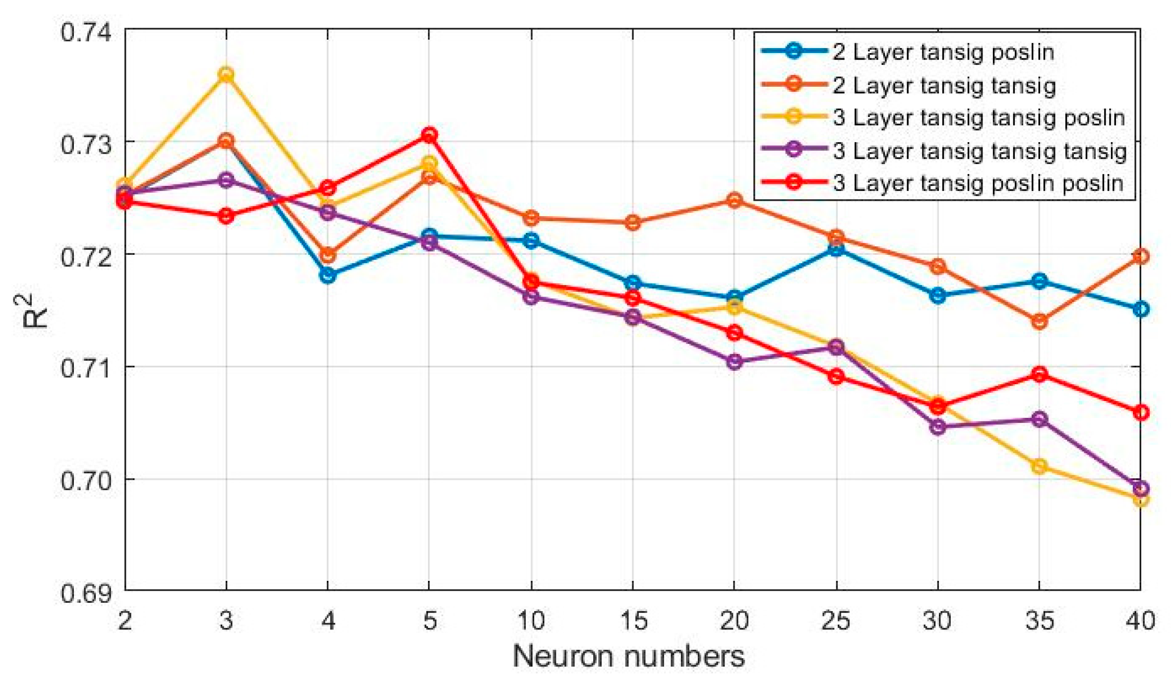
The OHC estimation accuracy is not only dependent on the choice of input features but is also closely related to the structure of the network. Therefore, it is necessary to study the sensitivity of the results to the ANN architecture, specifically to the number of hidden layers, the number of neurons in each layer, and the activation function . A grid-search approach was applied to find the optimized hyperparameters. Using a subset of test data from 2017, we compared the performance (quantified by R2) of networks with different hyperparameters (Figure 1).
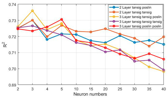
Figure 1.
Artificial neural network (ANN) performance measured in R2 of projecting OHC300 as a function of neuron numbers (x-axis). Different colors denote different combinations of hidden-layer numbers and activation functions. The training data is from 2005 to 2013 with a feature combination of Case 4 (see Table 1). The test data here is 12 months of 2017. In the legend, “tansig” means the tangential sigmoid activation function, while “poslin” means the Rectified Linear Unit (ReLU).
As Figure 1 demonstrates, when the number of neurons is less than five, the inversion result of a three-layer network is generally better than that of a two-layer network. However, when the number of neurons is greater than five, the inversion results of the two-layer network are better. With increasing numbers of neurons, the accuracy of OHC inversion in three-layer and two-layer networks increased first and then decreased. Three-layer networks generally present steep slopes, implying that these networks are more susceptible to overfitting. Therefore, maintaining a simple network structure is appropriate for the current problem, which is essentially extrapolating the target out of the training domain. Our previous application for the subsurface temperature with ANN came to a similar conclusion [25]. In general, increasing the number of hidden layers can effectively enhance the network’s fitting ability to complex input-to-output mapping functions. However, two downsides may emerge as the number of hidden layers increases: the data may be overfitted and the difficulty of training may increase dramatically, making it difficult for the model to converge.
In addition, the activation function is also an important influencing factor, as illustrated in Figure 1, which shows different combinations of activation functions. In our current MATLAB method, “tansig” indicates a tangential sigmoid activation function, while “poslin” indicates the Rectified Linear Unit. The OHC inversion results for two-layer networks indicate that the combination of tansig and poslin was not as good as tansig alone. Conversely, the result of the activation function containing poslin was better than the result of that containing tansig for all three-layer networks. In addition, it is expected that the poslin activation function will have better computation efficiency than tansig.
According to these tests, we selected a three-layer network with three neurons and a tansig–tansig–poslin structure as the optimized ANN architecture. By default, we report results using this architecture hereafter.
4.2. Optimization of Feature Combinations
The selection of remote sensing data as input features is crucial to retrieving the OHC. In the practice of machine learning, seeking a best feature combination is crucially important, yet such combinations are sometimes counterintuitive [40]. Therefore, features are often chosen in an ad hoc manner, a procedure sometimes called feature engineering. To optimize the feature combination, 16 experiments were designed as shown in Table 1. In these experiments, the data from the 12 months of 2010 were used to train the ANN model; then, the OHC300 in January 2011 was hindcasted with the tuned models and compared to the labeled data. For Case A in Table 1, during model training the first-level Argo data were treated as the “surface” features, which correspond to the 0-m depth for the current product. The R2 and RRMSE values are also reported in Table 1. Note that tests on other temporal snapshots yielded similar conclusions.
The retrieval results of the two data sources for Case 1 in Table 1 verify that SSH anomaly (SSHA) and SST anomaly (SSTA) are the main influencing factors of OHC. Cases 1A and 1R indicate that the accuracy of the two sources is fairly good with ~70% of the variance explained by the network; however, the accuracy of the satellite data inversion is relatively better. A comparison of Cases 1 and 2 indicates that the addition of latitude, longitude, and time information significantly improves the training for both data sources. This is consistent with previous subsurface temperature retrieval studies. A comparison of Cases 1 and 3 or Cases 2 and 4 suggests that the inclusion of SSW can improve the estimation accuracy but only marginally (~1%). Comparing Cases 1 and 5 shows that the salinity has a suppression effect (~6%) on the accuracy of the retrieval from the Argo data but increases that of Case R very slightly. This is due to the fact that the Argo SSS is inconsistent with the satellite-observed SSS. In particular, when using the salinity of the measured data to train and that of the satellite data to predict, the accuracy of the inversion is moderately reduced. In general, the inversion accuracy of Case R is better than that of Case A, which demonstrates that the use of satellite remote sensing data to build models is a more robust practice. Of all the cases, Case 8R has the highest accuracy (~80% variance reconstructed); however, considering the availability of SSS data, the feature combination in Case 4R was therefore selected for the following hindcast.
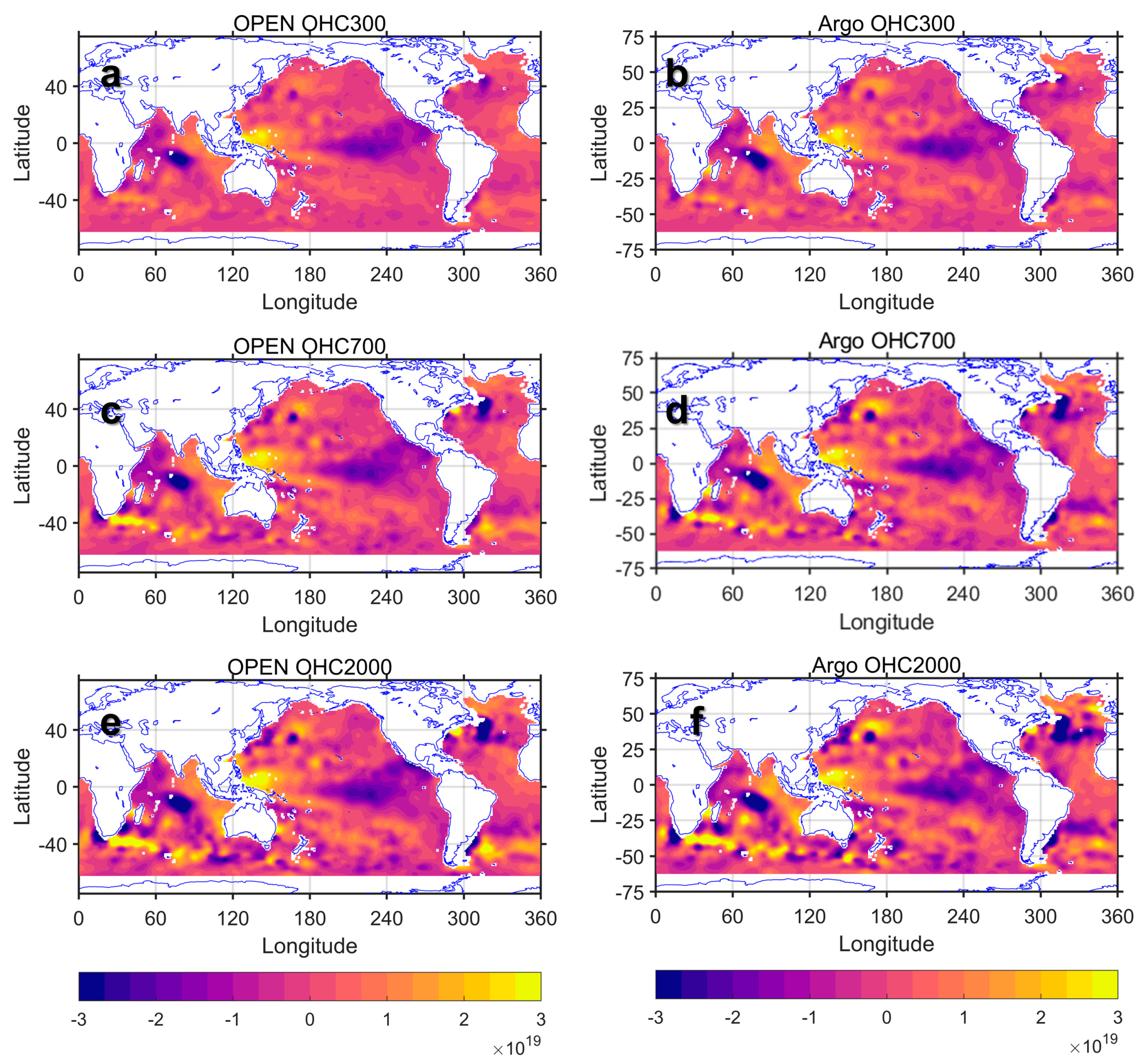
Figure 2 presents a comparison of the Argo-derived and OPEN OHC300, OHC700, and OHC2000 anomalies for one particular time snapshot (January 2011, as in Table 1). The retrieval R2 values of the three different depth ranges were 0.80, 0.82, and 0.80, respectively. The corresponding RRMSE values were 0.36, 0.34, and 0.37, respectively. The spatial distribution hindcasted by the ANN model for the three different depth ranges closely agrees with the Argo OHC. The small changes in the performance with depth suggest the robustness of ANN networks. The spatial distribution of the OHC reflects the El Niño–Southern Oscillation (ENSO) phenomenon. OHC presents abnormally high values in the tropical Indo-Pacific oceans; conversely, low OHC occurs in the eastern tropical Pacific. Alternating warming and cooling patterns gradually become apparent, reflecting the meandering of the Agulhas retroflection currents [41]. The spatial distributions of the three different depth ranges are consistent; however, the magnitude of the change in the heat content is different. The intensity of the change in the heat content gradually increases with depth through the three depths. The differences between OHC300 and OHC2000 are the most significant. For 0–300 m, the areas with significant OHC changes are primarily concentrated in the Pacific and Indian oceans. For 0–2000 m, OHC changes occur in all four oceans.
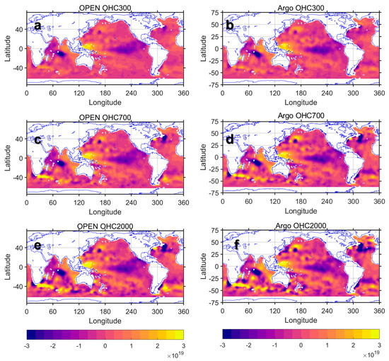
Figure 2.
The ocean heat content (OHC) (unit: Joule) at three depths (top: 0–300 m; middle: 0–700 m; bottom: 0–2000 m) for (left) OPEN-hindcasted and (right) Argo data in January 2011. The network was trained with 12-month data from 2010.
4.3. Data Reconstruction
Multiple experiments have proved the robustness and accuracy of the method in retrieving the OHC; therefore, in this section we formally trained the model using data from 2005 to 2018 with the ensemble technique and hindcasted the OHC to 1993. Various aspects of OPEN OHC data are compared with the five datasets, i.e., IAP, EN4, NCEI, GLORYS2V4, and ARMOR3D.
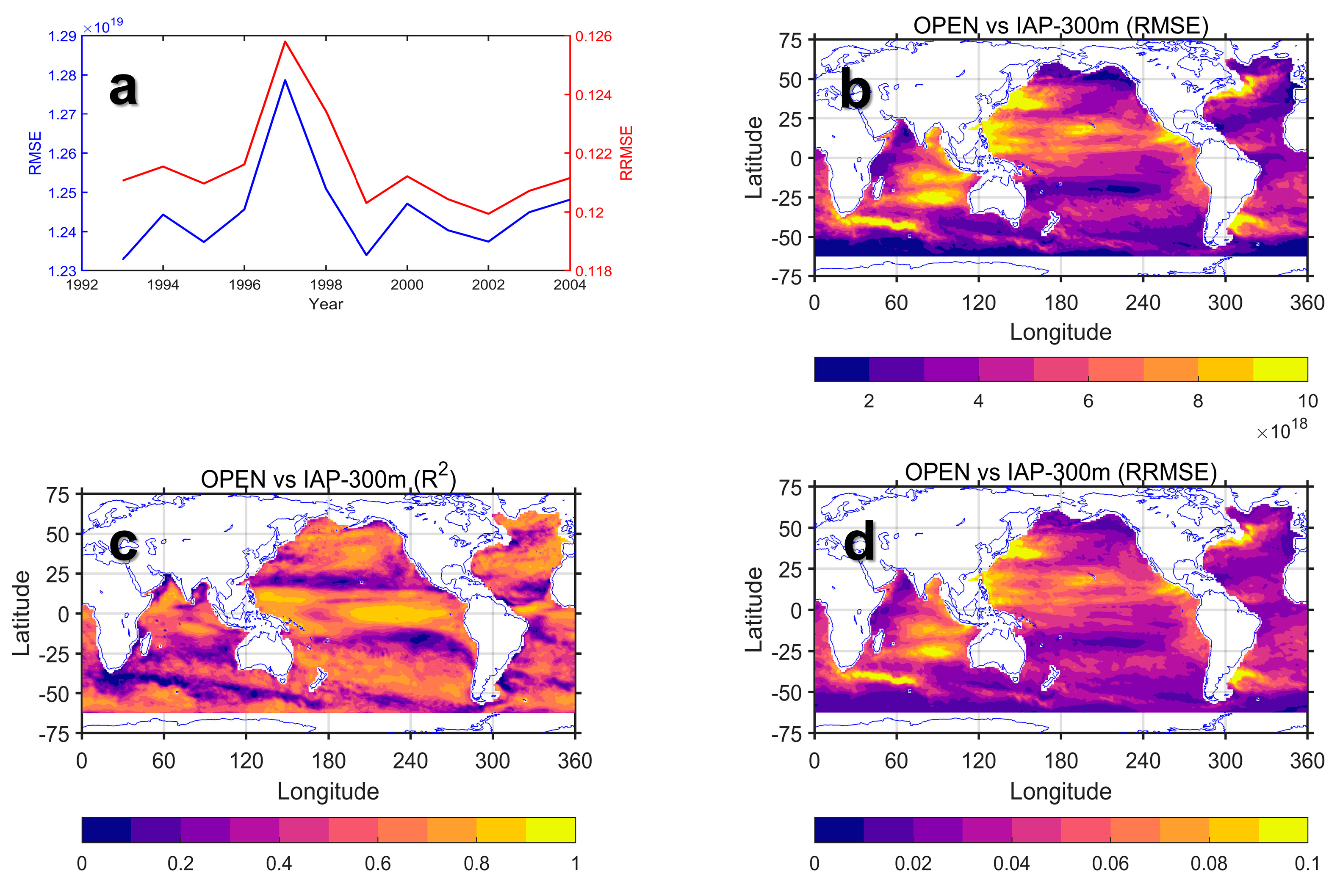
Figure 3a shows the accuracy of the OPEN-hindcasted 1993–2004 OHC compared to the IAP data. In Figure 3b–d, spatial correlation and error of OPEN OHC300 were analyzed against IAP data. The overall R2 was larger than 0.98, while RRMSE was 12%. The interannual variations in R2 and RRMSE were very small, suggesting a stable performance. The performance shows a very small trend. This is desirable for long-term projections. There is an abnormal signal in 1997 and 1998, which is likely related to the strong ENSO events in these years. ENSO may disturb the signal on the ocean surface, resulting in a deviation from the relationship learned by the network.
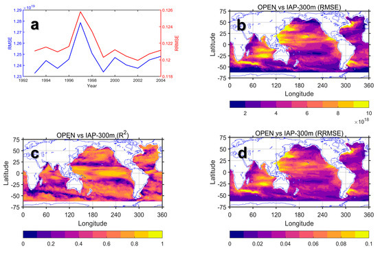
Figure 3.
Hindcasted OPEN OHC300 accuracy against the Institute of Atmospheric Physics (IAP) summarized in (a) different years from 2014 to 2018; and in (b–d) spatial maps of temporal correlation (c measured in R2) and errors (measured in b RMSE and d RRMSE with respect to a universal value of standard deviation).
Over space, the performance of OPEN presents a heterogeneous pattern. The R2 is generally high except for some narrow bands in the Antarctic Circumpolar Currents, two zonal 25° bands across the entire Pacific basin in both hemispheres, and in the Western Boundary Current Extensions. These regions are also characterized by high RMSE. Generally, the error accounts for ~10% of the spatio-temporal standard deviation of OHC300.
Compared to the Argo OHC for the full period at all depths, the R2 values are all larger than 0.988 (0.993, 0.988, 0.988, and 0.989 for OHC300, OHC700, OHC1500, and OHC2000, respectively), while the RRMSE values are all smaller than 0.111 (0.09, 0.109, 0.111, and 0.106, respectively). With the IAP data, the errors are larger (0.984, 0.971, 0.958, and 0.953 for R2 and 0.120, 0.158, 0.191, and 0.203 for RRMSE for OHC300, OHC700, OHC1500, and OHC2000, respectively), partially due to the uncertainty associated with a longer time span. It is worth mentioning that OPEN agrees with other products better than that with IAP (Supplementary Tables S1–S4). A best agreement between OPEN and EN4 product can be seen. In summary, the overall accuracy of the OPEN model is high. Therefore, the OPEN reconstruction can be extended to the period of 1993–2004.
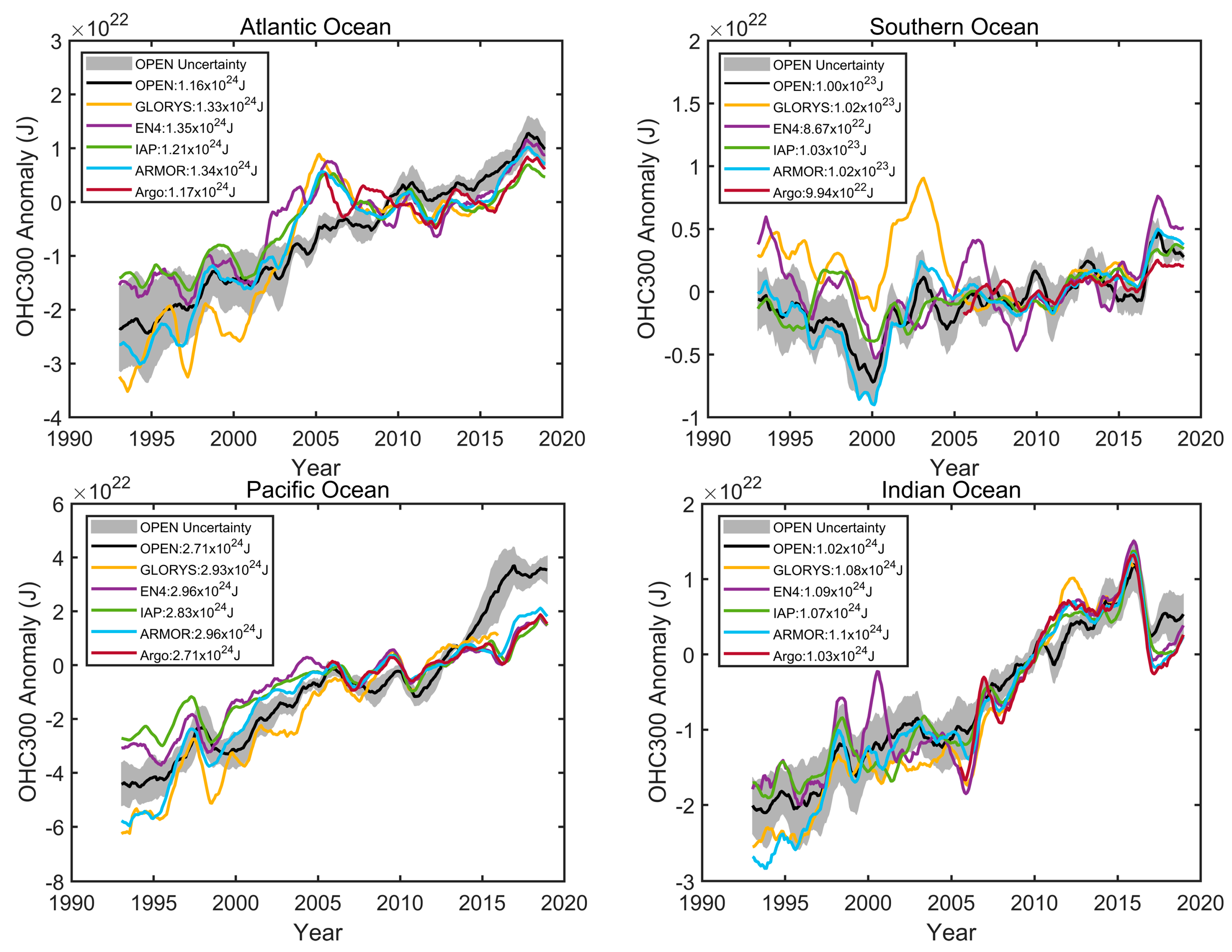
Figure 4 shows the OHC300 in all products, while the linear trends for the two time periods (1993–2010 and 1998–2015) are listed in Table 2. Comparisons of other depths can be found in the Supplementary Figures S1–S6. The overall trends reflect the continuous warming of the global ocean. In 2018 and 2019, the OHC reached a record high [11,42]. This further emphasizes the importance of quantifying the OHC, which is of great significance to understanding ocean warming and ocean heat transfer. OPEN OHC shows an abrupt bump in 1997 and 1998, presumably due to ENSO effects. This signal is readily apparent for deeper integrations (0–700, 0–1500, and 0–2000 m) while it is less prominent for 0–300 m. This makes sense because the OHC300 is more sensitive to surface signals. In Table 2, the warming rates of OPEN are higher than those of IAP during the same period. Two mapping-based datasets (EN4 and IAP) present very close trends and variabilities especially in the upper 300 m, while for deep integrals the divergence is large. In these depths, ARMOR3D and GLORYS2V4 present even larger trends. From Figure 4, it is apparent that OPEN falls well within the range of all other datasets. Its variation is mostly similar to those of ARMOR3D and GLORYS2V4 data except for the early 1990s. This makes sense since these three datasets incorporated similar sources of data, whereas EN4, IAP, and NCEI used different observation-based data.
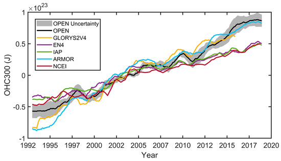
Figure 4.
Near-global OHC300 (unit: Joule) excluding polar regions. The anomaly is with respect to 1993–2015 period. All datasets were smoothed with a one-year moving average. Before the moving average procedure, seasonal cycles averaged from the first or last three years were respectively padded to the time-series. The name of each product is shown in the legend. For OPEN, ensemble-mean is shown in the black line, while the uncertainty was estimated by taking three standard deviations across six ensemble members. Notice that the National Centers for Environmental Information (NCEI) has a three-month temporal resolution, while all other datasets are monthly.

Table 2.
Warming rates of the global ocean OHC at different depths in ×1022 J/decade.
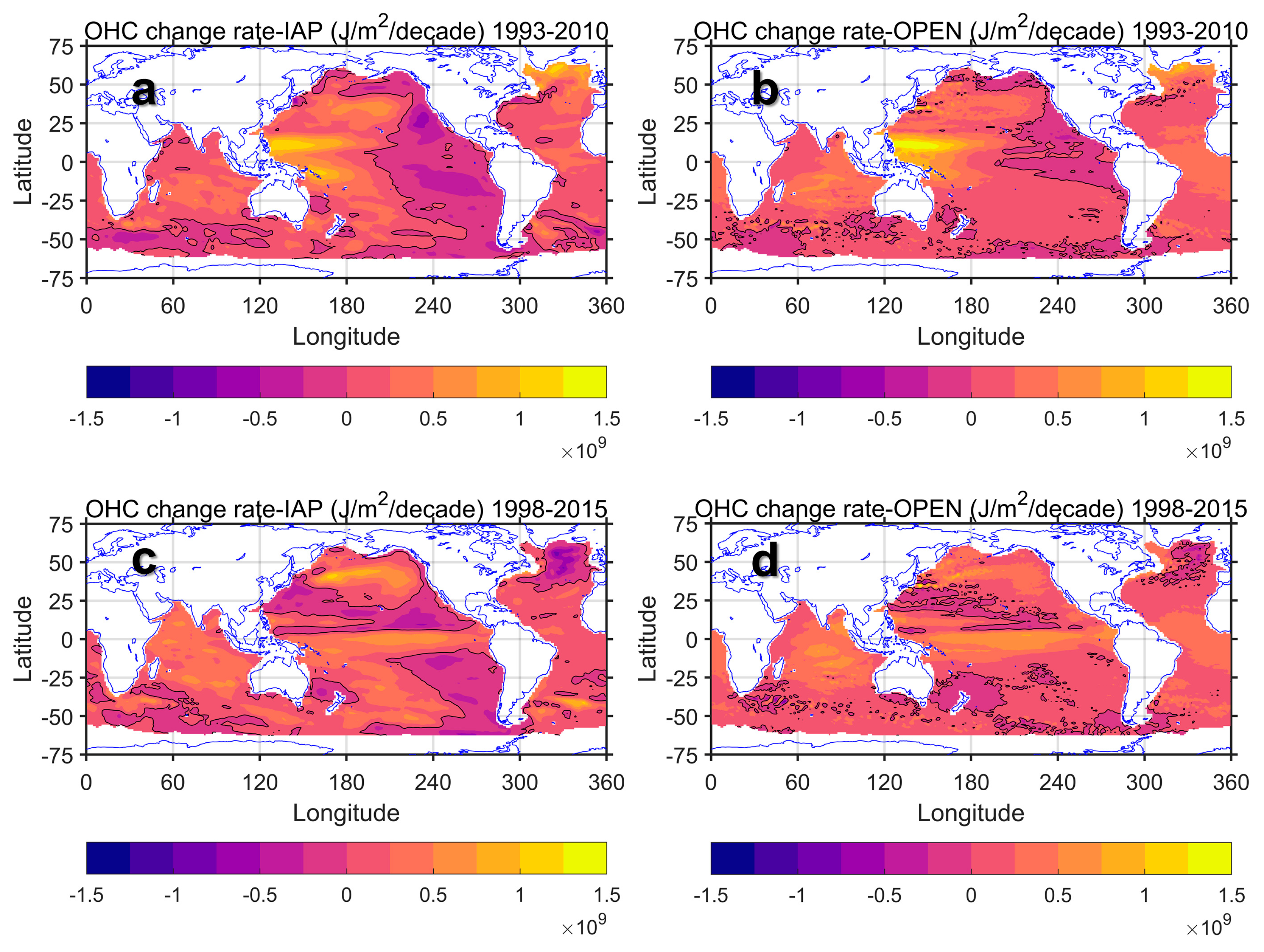
To further compare, we examined the OHC300 and its trends in different ocean basins (Figure 5 and Table 3) and the geographic distribution of the linear trends (Figure 6). Those figures for other depths can be found in the Supplementary. The warming trends of the four oceans present consistency to some degree. During these two periods, the highest ocean warming rate is concentrated in the Indo-Pacific oceans, which is consistent with the findings of Lee et al. [34], and the lowest warming rate is found in the Southern Ocean. As can be seen from the two datasets in Figure 6, the warming of OPEN and IAP from 1993 to 2010 are concentrated in the western Pacific region, with an opposite trend in the east. This agrees with the recent shift of the Pacific Decadal Oscillation to a negative phase [43]. During the latter period, both datasets present large spatial uncertainties in the warming trends, except for the overall warming in the Indian Ocean. The inconsistency in OPEN is largest in the Pacific Ocean, while is relatively small in other basins. In the late 2010s, an unexpected elevation is shown in the Pacific OHC in OPEN. This signal is not visible in Figure 4. About half of this inconsistency is associated with the different references between OPEN and other datasets (especially for ARMOR3D and GLORYS2V4, not shown in figures). On the other hand, it is noticeable that the uncertainty (gray envelop) of OPEN OHC300 is relatively small in the Pacific basin (compared with the data range in Figure 5). This implies that this inconsistency is systematic instead of random. A more physically consistent neural network approach might be required to improve this flaw. As in our previous contribution [25], one strategy is to use a clustering technique to narrow down sampling space and train different networks for different ocean current regimes. Another possible solution is to use a deeper neural network which can be more capable to extract the complex relationship between surface variables and OHC. This will be tackled in future studies.
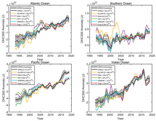

Table 3.
Warming rates of OHC300 for different ocean basins in ×1022 J/decade.
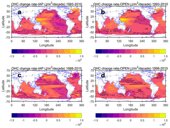
Figure 6.
The warming trends of the (a,c) IAP and (b,d) OPEN OHC300 in (a,b) 1993–2010 and (c,d) 1998–2015. Black contours are zero values.
The accuracy of the hindcasted OHC indicates the reliability and stability of the OPEN data. However, noting that, during the Argo period IAP presents some higher averages (~10%) than the Argo data and the OPEN product (Figure 5). To examine this phenomenon, we present OHC300 (non-anomaly) for the three datasets in April 2018 as an example (Figure 7). Even though the three products show very similar structures, the OHC in the IAP is apparently higher than the values of OPEN and Argo, particularly discernable in the subtropical gyres of the Pacific Ocean. This suggests a systematic warm bias in the IAP. This is likely because the IAP data include both Argo and XBT observations. Even though an advanced time-varying correction was applied to the XBT measurements, there is still a substantial warm bias in these measurements compared to more accurate CTD measurements [44,45]. This bias (~0.5 °C) is inevitably reflected in the value of the global OHC, even though the estimation of long-term (particularly in our case, recent decades) trends is less likely to be affected. Nevertheless, these uncertainties emphasize the importance of more independent OHC datasets.

Figure 7.
The spatial distribution of OHC300 (non-anomaly, unit: Joule) in (a) Argo, (b) IAP, and (c) OPEN in April 2018.
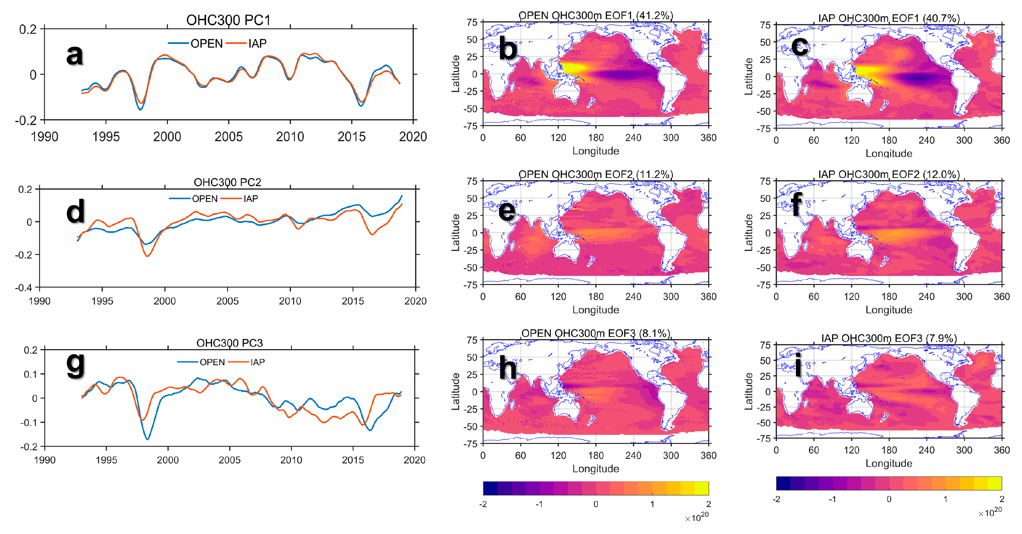
To further demonstrate the capability of OPEN to capture the spatial-temporal variability of the OHC, an empirical orthogonal function (EOF) analysis was applied to the two OHC products. The EOF analysis was conducted on the global OHC data after removing the linear trends and seasonal signals (using a 12-month moving average). Here we present OHC300 versus IAP data as an example (Figure 8), while those for other datasets can be found in the Supplementary Figures S7–S9. From Figure 8, we can see that OPEN presents high agreement with the IAP data. For the first mode, the PCs of the two products show only subtle differences (Figure 8a) with very similar explained variabilities (41.2% in IAP versus 40.7% in OPEN). The EOFs are also highly similar, particularly in the tropical Pacific, with a dipole structure in the western and eastern Pacific. Beyond the tropical ocean, some dissimilarities occur in the northern mid-latitudes of the Pacific. These suggest that OPEN correctly captures the leading mode, which is actually the ENSO-related mode, of the OHC. The second and third leading modes show slightly more inconsistencies but are still within a few percent. Further examinations of other modes and depth integrals all suggest that OPEN OHC captures the variability well compared to the IAP data. Together, these analyses indicate the validity of the OPEN OHC product.
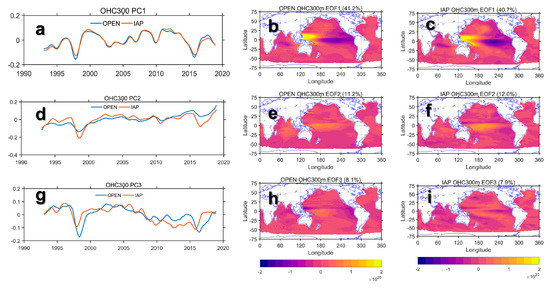
Figure 8.
EOF analysis on OHC300. From top to bottom are mode 1 (a–c), mode 2 (d–f), and mode 3 (g–i). From left to right are (a,d,g) time coefficients (or Principal Components, PCs), (b,e,h) spatial patterns (or EOFs) of OPEN data, and (c,f,i) EOFs of IAP data. The explained percentage of each mode is listed above the corresponding EOFs. Before EOF analysis, linear trends were first removed from the OHC data, and then seasonal signals were also removed with a 12-month moving average.
5. Summary and Conclusions
In this study, we presented a new ocean heat content product, i.e., the OPEN OHC product. OPEN OHC was trained using 1° gridded Argo OHC data and a set of remote sensing data including SST, SSH, SSW, and spatial and temporal information. Four ANNs were trained to approximate OHC integrated to four depths (namely, from the surface to 300, 700, 1500, and 2000 m) from these remote sensing data. We trained and optimized these ANNs using the data from 2005 to 2018 to enable a temporal extrapolation of the OHC. In particular, the architecture and feature combination of the ANNs were optimized via a series of sensitivity experiments. These experiments indicated that a simple network architecture (i.e., three hidden layers with three neurons in each layer) could facilitate the projection and hindcast of the OHC, yielding a final optimized network with R2 and RRMSE values of 0.8 and 0.3, respectively. Using the optimized networks, the full-range monthly OHC product at 1° × 1° from 1993 to 2018 for the four depths was hindcasted with high accuracy (R2 > 0.95 and RRMSE < 0.20). By using an ensemble technique, the uncertainty from the training could be estimated. By further comparison with five near-global OHC datasets using very different methodologies, we showed that the OPEN product reasonably reconstructed the variability of OHC, especially in the leading modes identified in the EOF analysis. The linear trends agreed with other datasets to a lesser extent but still showed considerable consistency in the trends across different ocean basins.
For any machine learning approach, the quality of training data determines the upper limit of its performance. In our case, gridded Argo data is indeed subjected to interpolation errors, especially in the boundary current regions [46] where the variability of ocean dynamic is intense, or in high latitudes that Argo is less capable to cover. The heterogeneous distribution of Argo profiles also partially contributes to these errors. On the other hand, numerical models also suffer from uncertainties associated with modeling techniques or imperfect representations of model physics. Globally, there still exist some misfits between the model data (GLORYS2V4) and other three observation-based datasets, even though state-of-art assimilation techniques were applied in GLORYS2V4 modeling. In this regard, one perspective is that although any individual dataset (even an observation-based one) inevitably contains some degree of uncertainty, the composite/ensemble of multi-source data can better represent the global thermodynamics. Therefore, one future direction is to dig into multiple datasets, especially into vast model data that are driven by physics with better dynamical consistency.
Various previous studies have highlighted the necessity of more independent OHC products [29,47] to extend our understanding of the Earth’s climate system. Indeed, there is a lack of quality ocean subsurface data prior to 2005. Most previous datasets were obtained from the mapping of historical observations with discrete sampling in time and space. This may introduce systematic biases when analyzing the variabilities and trends of the ocean. Nevertheless, the data products obtained by using different methodologies (such as mapping-based NCEI, IAP, and EN4 when compared with model-based GLORYS2V4 data) have substantially different spatiotemporal variances. With such inconsistent datasets, different conclusions may be drawn. This hinders our understanding of recent climate changes. In this regard, our OPEN data could provide a good complement to the list of available OHC products to help improve our understanding of the redistribution of oceanic heat, although further related studies should be conducted in the future.
Supplementary Materials
The following are available online at https://www.mdpi.com/2072-4292/12/14/2294/s1, Figure S1 Near-global OHC700; Figure S2 Same as Figure S1, but for OHC1500; Figure S3 Same as Figure S1, but for OHC2000; Figure S4 OHC700 of four ocean basins from 1993 to 2018; Figure S5 Same as Figure S4, but for OHC1500; Figure S6 Same as Figure S4, but for OHC2000; Figure S7 EOF analysis on OHC300 for EN4 and OPEN; Figure S8 Same as Figure S7, but for OPEN and ARMOR; Figure S9 Same as Figure S7, but for OPEN and GLORYS2V4; Table S1: Accuracy comparison between OPEN data and other data for 0–300 meters, Table S2: Accuracy comparison between OPEN data and other data for 0–700 meters, Table S3: Accuracy comparison between OPEN data and other data for 0–1500 meters, Table S4: Accuracy comparison between OPEN data and other data for 0–2000 meters.
Author Contributions
Conceptualization, H.S. and W.L.; methodology, H.Z. and W.L.; validation, H.Z. and W.L.; formal analysis, H.Z. and W.L.; investigation, H.S., H.Z., and W.L.; resources, H.S., H.Z., and X.G.; data curation, H.Z. and W.L.; writing—original draft preparation, H.Z.; writing—review and editing, H.S., H.Z., X.G., and W.L.; visualization, H.Z., T.Q., and W.L.; supervision, X.-H.Y., X.G., and W.L.; and funding acquisition, X.-H.Y., H.S. and W.L. All authors have read and agreed to the published version of the manuscript.
Funding
This research was funded by National Natural Science Foundation of China (Grant Numbers: 41906019, 41971384) and China Postdoctoral Science Foundation (2019M652245). It was also funded by SOA Global Change and Air-Sea Interaction Project (Grant Numbers: GASI-02-PAC-YGST2-02 and GASI-IPOVAI-01-04), the National Natural Science Foundation of China (41961144011, 91858202 and 41630963) and the National Key R&D Program of China (2019YFA0606702).
Acknowledgments
The authors would like to thank two anonymous reviewers for their constructive comments, which significantly improved the quality of our paper. The OPEN dataset and corresponding codes will be opened, as its name suggests, to the research community at https://github.com/scenty/OPEN-OHC. The colormap was adopted from the Perceptually uniform colormaps by Ander Biguri (https://www.mathworks.com/matlabcentral/fileexchange/51986-perceptually-uniform-colormaps, retrieved June 30, 2020) on MATLAB Central File Exchange website.
Conflicts of Interest
The authors declare no conflict of interest.
References
- Trenberth, K.E.; Fasullo, J.T.; Balmaseda, M.A. Earth’s Energy Imbalance. J. Clim. 2014, 27, 3129–3144. [Google Scholar] [CrossRef]
- Meyssignac, B.; Boyer, T.; Zhao, Z.; Hakuba, M.Z.; Landerer, F.W.; Stammer, D.; Köhl, A.; Kato, S.; L’Ecuyer, T.; Ablain, M.; et al. Measuring Global Ocean Heat Content to Estimate the Earth Energy Imbalance. Front. Mar. Sci. 2019, 6, 432. [Google Scholar] [CrossRef]
- Von Schuckmann, K.; Palmer, M.D.; Trenberth, K.E.; Cazenave, A.; Chambers, D.; Champollion, N.; Hansen, J.; Josey, S.A.; Loeb, N.; Mathieu, P.P.; et al. An imperative to monitor Earth’s energy imbalance. Nat. Clim. Chang. 2016, 6, 138–144. [Google Scholar] [CrossRef]
- Balmaseda, M.A.; Trenberth, K.E.; Källén, E. Distinctive climate signals in reanalysis of global ocean heat content. Geophys. Res. Lett. 2013, 40, 1754–1759. [Google Scholar] [CrossRef]
- Bindoff, N.L.; Willebrand, J.; Artale, V.; Cazenave, A.; Gregory, J.M.; Gulev, S.; Hanawa, K.; Le Quere, C.; Levitus, S.; Nojiri, Y.; et al. Observations: Oceanic climate change and sea level. In Climate Change 2007: The Physical Science Basis; Cambridge University Press: Cambridge, UK, 2007. [Google Scholar]
- Antonov, J.I.; Levitus, S.; Boyer, T.P. Climatological annual cycle of ocean heat content. Geophys. Res. Lett. 2004, 31, L04304. [Google Scholar] [CrossRef]
- Levitus, S.; Antonov, J.I.; Wang, J.; Delworth, T.L.; Dixon, K.W.; Broccoli, A.J. Anthropogenic Warming of Earth’s Climate System. Science 2001, 292, 267–270. [Google Scholar] [CrossRef] [PubMed]
- IPCC. Observations: Ocean Pages. In Climate Change 2013—The Physical Science Basis: Working Group I Contribution to the Fifth Assessment Report of the Intergovernmental Panel on Climate Change; Cambridge University Press: Cambridge, UK, 2014; pp. 255–316. [Google Scholar] [CrossRef]
- Rebert, J.P.; Donguy, J.R.; Eldin, G.; Wyrtki, K. Relations between sea-level, thermocline depth, heat-content, and dynamic height in the tropical pacific-ocean. J. Geophys. Res. Oceans 1985, 90, 1719–1725. [Google Scholar] [CrossRef]
- Chen, J.L.; Shum, C.K.; Wilson, C.R.; Chambers, D.P.; Tapley, B.D. Seasonal sea level change from TOPEX/Poseidon observation and thermal contribution. J. Geod. 2000, 73, 638–647. [Google Scholar] [CrossRef]
- Cheng, L.J.; Abraham, J.; Zhu, J.; Trenberth, K.E.; Fasullo, J.; Boyer, T.; Locarnini, R.; Zhang, B.; Yu, F.J.; Wan, L.Y.; et al. Record-Setting Ocean Warmth Continued in 2019. Adv. Atmos. Sci. 2020, 37, 137–142. [Google Scholar] [CrossRef]
- Klemas, V.; Yan, X.H. Subsurface and deeper ocean remote sensing from satellites: An overview and new results. Prog. Oceanogr. 2014, 122, 1–9. [Google Scholar] [CrossRef]
- Akbari, E.; Alavipanah, S.K.; Jeihouni, M.; Hajeb, M.; Haase, D.; Alavipanah, S. A Review of Ocean/Sea Subsurface Water Temperature Studies from Remote Sensing and Non-Remote Sensing Methods. Water 2017, 9, 936. [Google Scholar] [CrossRef]
- Su, H.; Wu, X.; Yan, X.-H.; Kidwell, A. Estimation of subsurface temperature anomaly in the Indian Ocean during recent global surface warming hiatus from satellite measurements: A support vector machine approach. Remote Sens. Environ. 2015, 160, 63–71. [Google Scholar] [CrossRef]
- Yan, X.H.; Schubel, J.R.; Pritchard, D.W. Ocean upper mixed layer depth determination by the use of satellite data. Remote Sens. Environ. 1990, 32, 55–74. [Google Scholar] [CrossRef]
- Chu, P.C.; Fan, C.; Liu, W.T. Determination of Vertical Thermal Structure from Sea Surface Temperature. J. Atmos. Ocean. Technol. 2000, 17, 971–979. [Google Scholar] [CrossRef]
- Yan, X.H.; Okubo, A.; Schubel, J.R.; Pritchard, D.W. An analytical model for remote-sensing determination of the mixed layer depth. Deep Sea Res. Part A Oceanogr. Res. Pap. 1991, 38, 267–287. [Google Scholar] [CrossRef]
- Reichstein, M.; Camps-Valls, G.; Stevens, B.; Jung, M.; Denzler, J.; Carvalhais, N. Deep learning and process understanding for data-driven Earth system science. Nature 2019, 566, 195–204. [Google Scholar] [CrossRef]
- Ali, M.M.; Swain, D.; Weller, R.A. Estimation of ocean subsurface thermal structure from surface parameters: A neural network approach. Geophys. Res. Lett. 2004, 31, L20308. [Google Scholar] [CrossRef]
- Jain, S.; Ali, M.M. Estimation of Sound Speed Profiles Using Artificial Neural Networks. IEEE Geosci. Remote Sens. Lett. 2006, 3, 467–470. [Google Scholar] [CrossRef]
- Swain, D.; Ali, M.M.; Weller, R.A. Estimation of mixed-layer depth from surface parameters. J. Mar. Res. 2006, 64, 745–758. [Google Scholar] [CrossRef]
- Jain, S.; Ali, M.M.; Sen, P.N. Estimation of sonic layer depth from surface parameters. Geophys. Res. Lett. 2007, 34, L17602. [Google Scholar] [CrossRef]
- Jagadeesh, P.S.V.; Kumar, M.S.; Ali, M.M. Estimation of Heat Content and Mean Temperature of Different Ocean Layers. IEEE J. Sel. Top. Appl. Earth Obs. Remote Sens. 2015, 8, 1251–1255. [Google Scholar] [CrossRef]
- Guinehut, S.; Dhomps, A.L.; Larnicol, G.; Le Traon, P.Y. High resolution 3-D temperature and salinity fields derived from in situ and satellite observations. Ocean Sci. 2012, 8, 845–857. [Google Scholar] [CrossRef]
- Lu, W.; Su, H.; Yang, X.; Yan, X.-H. Subsurface temperature estimation from remote sensing data using a clustering-neural network method. Remote Sens. Environ. 2019, 229, 213–222. [Google Scholar] [CrossRef]
- Charantonis, A.A.; Badran, F.; Thiria, S. Retrieving the evolution of vertical profiles of Chlorophyll-a from satellite observations using Hidden Markov Models and Self-Organizing Topological Maps. Remote Sens. Environ. 2015, 163, 229–239. [Google Scholar] [CrossRef]
- Friedrich, T.; Oschlies, A. Neural network-based estimates of North Atlantic surface pCO2 from satellite data: A methodological study. J. Geophys. Res. Oceans 2009, 114, C03020. [Google Scholar] [CrossRef]
- Garcia-Gorriz, E.; Garcia-Sanchez, J. Prediction of sea surface temperatures in the western Mediterranean Sea by neural networks using satellite observations. Geophys. Res. Lett. 2007, 34, L11603. [Google Scholar] [CrossRef]
- Zanna, L.; Khatiwala, S.; Gregory, J.M.; Ison, J.; Heimbach, P. Global reconstruction of historical ocean heat storage and transport. Proc. Natl. Acad. Sci. USA 2019, 116, 1126–1131. [Google Scholar] [CrossRef]
- Roemmich, D.; Gilson, J. The 2004–2008 mean and annual cycle of temperature, salinity, and steric height in the global ocean from the Argo Program. Prog. Oceanogr. 2009, 82, 81–100. [Google Scholar] [CrossRef]
- Su, H.; Wu, X.B.; Lu, W.F.; Zhang, W.W.; Yan, X.H. Inconsistent Subsurface and Deeper Ocean Warming Signals During Recent Global Warming and Hiatus. J. Geophys. Res. Oceans 2017, 122, 8182–8195. [Google Scholar] [CrossRef]
- Yan, X.-H.; Boyer, T.; Trenberth, K.; Karl, T.R.; Xie, S.-P.; Nieves, V.; Tung, K.-K.; Roemmich, D. The global warming hiatus: Slowdown or redistribution? Earth’s Future 2016, 4, 472–482. [Google Scholar] [CrossRef]
- Chen, X.Y.; Tung, K.K. Varying planetary heat sink led to global-warming slowdown and acceleration. Science 2014, 345, 897–903. [Google Scholar] [CrossRef] [PubMed]
- Lee, S.-K.; Park, W.; Baringer, M.O.; Gordon, A.L.; Huber, B.; Liu, Y. Pacific origin of the abrupt increase in Indian Ocean heat content during the warming hiatus. Nat. Geosci. 2015, 8, 445–449. [Google Scholar] [CrossRef]
- Cheng, L.; Trenberth, K.E.; Fasullo, J.; Boyer, T.; Abraham, J.; Zhu, J. Improved estimates of ocean heat content from 1960 to 2015. Sci. Adv. 2017, 3, e1601545. [Google Scholar] [CrossRef] [PubMed]
- Levitus, S.; Antonov, J.I.; Boyer, T.P.; Baranova, O.K.; Garcia, H.E.; Locarnini, R.A.; Mishonov, A.V.; Reagan, J.R.; Seidov, D.; Yarosh, E.S.; et al. World ocean heat content and thermosteric sea level change (0–2000 m), 1955–2010. Geophys. Res. Lett. 2012, 39, L10603. [Google Scholar] [CrossRef]
- Good, S.A.; Martin, M.J.; Rayner, N.A. EN4: Quality controlled ocean temperature and salinity profiles and monthly objective analyses with uncertainty estimates. J. Geophys. Res. Oceans 2013, 118, 6704–6716. [Google Scholar] [CrossRef]
- Gouretski, V.; Reseghetti, F. On depth and temperature biases in bathythermograph data: Development of a new correction scheme based on analysis of a global ocean database. Deep Sea Res. Part I Oceanogr. Res. Pap. 2010, 57, 812–833. [Google Scholar] [CrossRef]
- Foresee, F.D.; Hagan, M.T. Gauss-Newton Approximation to Bayesian Learning. In Proceedings of the International Conference on Neural Networks, Houston, TX, USA, 12 June 1997. [Google Scholar]
- Su, H.; Yang, X.; Lu, W.; Yan, X.-H. Estimating Subsurface Thermohaline Structure of the Global Ocean Using Surface Remote Sensing Observations. Remote Sens. 2019, 11, 1598. [Google Scholar] [CrossRef]
- Beal, L.M.; De Ruijter, W.P.; Biastoch, A.; Zahn, R. On the role of the Agulhas system in ocean circulation and climate. Nature 2011, 472, 429–436. [Google Scholar] [CrossRef]
- Cheng, L.J.; Abraham, J.; Hausfather, Z.; Trenberth, K.E. How fast are the oceans warming? Science 2019, 363, 128–129. [Google Scholar] [CrossRef]
- Mantua, N.J.; Hare, S.R.; Zhang, Y.; Wallace, J.M.; Francis, R.C. A Pacific interdecadal climate oscillation with impacts on salmon production. Bull. Am. Meteorol. Soc. 1997, 78, 1069–1080. [Google Scholar] [CrossRef]
- Levitus, S.; Antonov, J.I.; Boyer, T.P.; Locarnini, R.A.; Garcia, H.E.; Mishonov, A.V. Global ocean heat content 1955–2008 in light of recently revealed instrumentation problems. Geophys. Res. Lett. 2009, 36, L07608. [Google Scholar] [CrossRef]
- Cheng, L.; Abraham, J.; Goni, G.; Boyer, T.; Wijffels, S.; Cowley, R.; Gouretski, V.; Reseghetti, F.; Kizu, S.; Dong, S.; et al. XBT Science: Assessment of Instrumental Biases and Errors. Bull. Am. Meteorol. Soc. 2016, 97, 924–933. [Google Scholar] [CrossRef]
- Jeong, Y.; Hwang, J.; Park, J.; Jang, C.J.; Jo, Y.H. Reconstructed 3-D Ocean Temperature Derived from Remotely Sensed Sea Surface Measurements for Mixed Layer Depth Analysis. Remote Sens. 2019, 11, 3018. [Google Scholar] [CrossRef]
- Resplandy, L.; Keeling, R.F.; Eddebbar, Y.; Brooks, M.; Wang, R.; Bopp, L.; Long, M.C.; Dunne, J.P.; Koeve, W.; Oschlies, A. Quantification of ocean heat uptake from changes in atmospheric O2 and CO2 composition. Sci. Rep. 2019, 9, 20244. [Google Scholar] [CrossRef]
© 2020 by the authors. Licensee MDPI, Basel, Switzerland. This article is an open access article distributed under the terms and conditions of the Creative Commons Attribution (CC BY) license (http://creativecommons.org/licenses/by/4.0/).

