Article

Recording Urban Land Dynamic and Its Effects during 2000–2019 at 15-m Resolution by Cloud Computing with Landsat Series

1
Key Laboratory of Wetland Ecology and Environment, Northeast Institute of Geography and Agroecology, Chinese Academy of Sciences, Changchun 130102, China
2
University of Chinese Academy of Sciences, Beijing 100049, China
3
Water and Hydraulic Survey and Planning Institute, Changchun 130021, China
4
College of Earth Sciences, Jilin University, Changchun 130012, China
5
Jilin Guoyao Geographic Information Technology Co., Ltd., Changchun 130061, China
*
Author to whom correspondence should be addressed.
These authors contributed equally to this work.
Remote Sens. 2020, 12(15), 2451; https://doi.org/10.3390/rs12152451
Submission received: 15 June 2020 / Revised: 22 July 2020 / Accepted: 28 July 2020 / Published: 30 July 2020

Abstract

:
Cities, the core of the global climate change and economic development, are high impact land cover land use change (LCLUC) hotspots. Comprehensive records of land cover land use dynamics in urban regions are essential for strategic climate change adaption and mitigation and sustainable urban development. This study aims to develop a Google Earth Engine (GEE) application for high-resolution (15-m) urban LCLUC mapping with a novel classification scheme using pan-sharpened Landsat images. With this approach, we quantified the annual LCLUC in Changchun, China, from 2000 to 2019, and detected the abrupt changes (turning points of LCLUC). Ancillary data on social-economic status were used to provide insights on potential drivers of LCLUC by examining their correlation with change rate. We also examined the impacts of LCLUC on environment, specifically air pollution. Using this approach, we can classify annual LCLUC in Changchun with high accuracy (all above 0.91). The change detection based on the high-resolution wall-to-wall maps show intensive urban expansion with the compromise of cropland from 2000 to 2019. We also found the growth of green space in urban regions as the result of green space development and management in recent years. The changing rate of different land types were the largest in the early years of the observation period. Turning points of land types were primarily observed in 2009 and 2010. Further analysis showed that economic and industry development and population migration collectively drove the urban expansion in Changchun. Increasing built-up areas could slow wind velocity and air exchange, and ultimately led to the accumulation of PM2.5. Our implement of pan-sharpened Landsat images facilitates the wall-to-wall mapping of temporal land dynamics at high spatial resolution. The primary use of GEE for mapping urban land makes it replicable and transferable by other users. This approach is a first crucial step towards understanding the drivers of change and supporting better decision-making for sustainable urban development and climate change mitigation.

1. Introduction

Urban areas, occupying no more than 3% of earth’s land, support the daily lives of 55% of the global population [1,2]. Rapid urban growth has led to considerable problems such as urban heat island, carbon emission, biodiversity loss, and pollution. Cities are now the central to climate change mitigation and sustainable development management. Achieving sustainable development goals requires the sustainable management of cities, which needs to untangle the complexities of the effects of urbanization on ecology, human health, and economy [3,4,5]. The fundamental for the sustainable management of cities is the understanding of urbanization history, namely land cover land use change (LCLUC), which is essential to explore the impacts of urbanization on environment.
Remote sensing, with the capability to provide long-term spatial information of land cover and land use (LCLU) [6,7,8,9,10,11], has been widely used to observe LCLUC. The development of remote sensing techniques, especially those of long-term satellites such as Landsat, provides a unique opportunity to track urban expansion through time [12]. Recent studies using Landsat images showed that urbanization was concentrated in the northern hemisphere during the past three decades, leading by China and the U.S. [6,11]. The map of continuous LCLU is particularly useful for evaluating change rate [13,14], for example, abrupt change, the key process in urbanization, can be detected with annual LCLU maps [15].
Understanding of the environmental problem in urban area can be facilitated by the detailed information of LCLUC. Urbanization consumed natural vegetation and cropland has resulted in many environmental and social problems [7,13,16,17]. The loss of natural vegetation is related to air pollution, urban heat island, and increasing respiratory diseases [16,17,18]. Urban expansion consumed cropland and degraded grain production, and thus threatens the food security of billions of people [19,20]. As cities are attracting more immigration and investments, sustainable management of cities needs detailed LCLUC through time and the associated consequences on the environment. Moreover, in-depth understanding needs high-resolution LCLU maps because of the high spatial heterogeneity in cities. For example, LCLUC based on 30-m observation lost the information of green space change [21], which could hinder the understanding of urban environment change. Meanwhile, long-term LCLUC at a large scale also requires efficient management of data and computing strategies. Google Earth Engine (GEE), a cloud-based geospatial processing computing platform, allows for geospatial data retrieval, processing, and analysis from local to planetary scale [22]. It makes it more efficient to monitor LCLUC by rapidly and accurately processing various amounts of satellite data [6,11,23,24,25].
It is possible to obtain long-term and high-resolution LCLUC maps with Landsat ETM+ and OLI, which provide a 15-m panchromatic band for sharpening multispectral bands since 1999 [12]. Using pan-sharpened Landsat data improved the urban LCLU classification [26,27]. Pan-sharpening methods are generally built-in functions of remote sensing platforms, such as Gram-Schmidt method and IHS method [28]. Other methods built by programming platforms, such as HSV transformation in Google Earth Engine, are also available for pan-sharpening [29]. However, the HSV is not efficient because only three spectral bands can be sharpened through one transformation. Sharpening all Landsat bands needs to apply HSV with multiple times, which hampers the construction of spectral indices to map LCLU. Currently, Landsat pan-sharpening with GEE has not been reported, remaining a pressing requirement for mapping LCLU with high resolution. An efficient method of Landsat pan-sharpening needs to be developed based on GEE.
Changchun City, China, has undergone significant urbanization in the past two decades [14,16,30]. Thanks to Soviet planning, in contrast to most cities in China, Changchun still has sufficient space for urban greening despite the artificial infrastructure that kept filling up the city [9,31]. Therefore, Changchun has been a laboratory to learn the relationship between LCLUC and urban ecology, especially how the ecosystem reacts to the warming climate. For example, the cooling-effect and emission-offset capacity of green space changes have been studied in this city [16,17]. However, the previous observation was conducted based on land use land cover at a multi-year interval, which is not sufficient to quantify the effects of land cover change on the temporal change of environment.
Driven by the demands of comprehensive records of urban land use land cover dynamics, this study aims to generate annual maps of urban LCLU at 15-m resolution by a multilevel decision rule method in GEE. This method would rely on a new Landsat pan-sharpening algorithm using GEE. The approach was applied to capture the annual change and turning point of LCLU in Changchun from 2000 to 2019. The LCLU maps were then used to further investigate the socio-economic drivers and environmental effects of LCLUC through statistical analysis. The implementation of our methods would help to acquire urban knowledge at a finer spatiotemporal resolution.

2. Materials and Methods

2.1. Study Area

Changchun, the major city in Northeast China, is the capital of Jilin province. The humid continental climate with the long cold winter governs the regional biomes, representing by temperate conifers. As lying in the continental plain of northeast Asia, Changchun became the modern city proto in China since the early 20th century due to railway construction by Russian and Japanese. As ordered by the central government, Changchun priorly developed heavy industrial and automobile manufacture from the 1950s. However, the economic depression in Changchun was impressed trail after the rapid development in coastal cities in recent decades. Winning the award of National Garden City in 2001 led Changchun to pay more attention to urban greenness, improving its livability and reputation. The built-up land and green space have filled Changchun (Figure 1). The long-term city development made Changchun an important laboratory to study urbanization and environmental change [17,31].

2.2. Landsat Series and Pan-Sharpening in GEE

Landsat sensors have been providing multispectral images since 1972, serving earth observation at 30-60 m resolution for decades. Because lapped acquisition from sensors made dense observations available (Table 1), TM images were applied to fill the gap of ETM+ images’ multispectral bands. The panchromatic band of the ETM+ and OLI sensors can apply to promote original bands to 15-m resolution, enhancing Landsat availability for urban study [26]. In GEE, to observe land dynamics, we employed Landsat top-of-atmosphere images (TOA) with the cloud cover <80% and the path/row of 128029, 128030, and 129030. The cloud-removing algorithm iterated all images, which were prepared to compose a yearly image by median stacking.
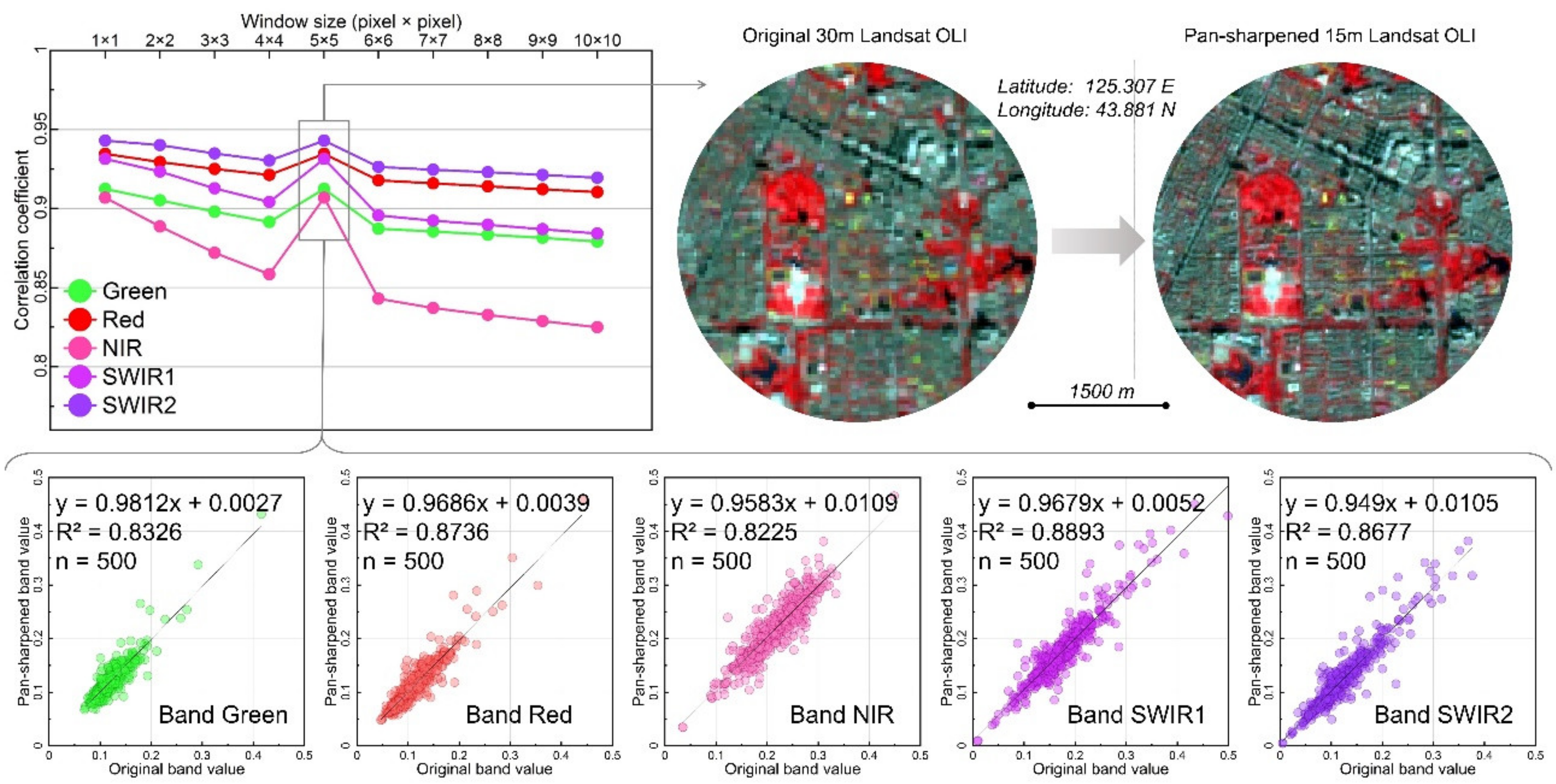
A new algorithm of GEE was developed for Landsat pan-sharpening in this study. The JavaScript-based HSV method is the built-in function of GEE, which can sharpen three bands through one transformation that includes two-step algorithms of rgbToHsv() and hsvToRgb() [29]. Instead of using the HSV, we directly reassigned multispectral information to up-scaled pixels based on a sliding pixel-window, including five steps (1) stacking all bands in one image, (2) forming a mean array by sliding the window, (3) recording the variation from multispectral mean to panchromatic mean, (4) recording the variation of multispectral information from original to mean, and (5) resigning multispectral information into 15-m pixels by multiplying pan band and two variations in each pixel. By testing, the 5 × 5 (or 150-m length) pixel-window could reserve the original multispectral information, which is evidenced by a Pearson coefficient of more than 0.9 in each band (Figure 2). As the pixel heterogeneity has been enhanced spatially, 15-m spectral indices could be obtained.
Spectral indices that include Normalized Difference Vegetation Index (NDVI) and Modified Normalized Difference Vegetation Index (MNDWI) were applied to extract LCLU pixels [32]. We further employed NDVI for phenology analysis by calibrating ETM+ and OLI images [33]. In addition, to avoid saturation of the NDVI, Fractional Vegetation Cover (FVC) calculated from NDVI was used for extracting vegetation.
NDVI = NIR - R / NIR + R
MNDWI = G - SWIR 1 / G + SWIR 1
FVC = NDVI - NDVI soil / NDVI veg + NDVI soil
where NDVI soil and NDVI veg denote the mean NDVI in bare ground and vegetation, respectively.

2.3. Integration of Automatic Thresholding and Multilevel Decision Rule Process

The urban LCLU category was defined by referencing peer-reviewed works [14,34,35] and visually investigating Google Earth images (Table 2). The difference is a category of green space that contains three vegetation types of forest, grass, and shrub. Although individual vegetation classes were not classified, our scheme was meeting the research need in Changchun [17,31,35] and avoided commission error between vegetation types due to lack of structure definitions.
A multilevel decision rule (MDR) algorithm was developed to generate urban LCLU maps by thresholding spectral index in this study. Despite machine learning classifiers are performing good LCLU classification [14,25], we aimed to timely obtain urban land information by saving the time taken in classifier debugging, sample collection, feature adjusting, etc. Previous studies indicated the effectiveness of decision rules, such as in mapping paddy rice and urban settlement [24,36]. Nonetheless, the multiple rules integration, namely MDR that orderly extracts LCLU [37,38], has not been effectively applied in GEE. This study applied and packaged MDR as an effective classifier in GEE to observe land dynamics, namely annual LCLUC [14].
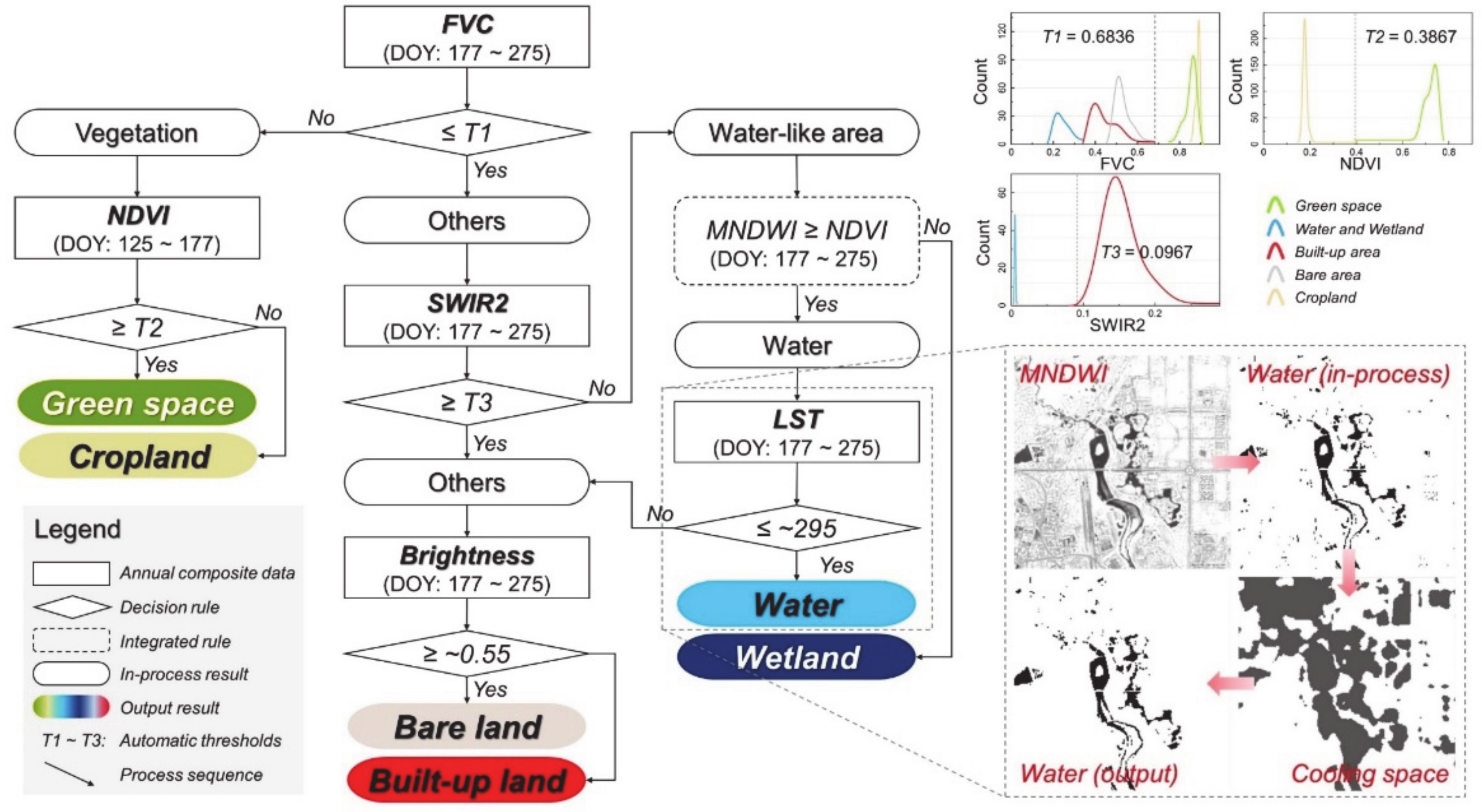
MDR sequence maps LCLU through analyzing spectra, phenology, and ecology (Figure 3). The vegetation extent was primarily extracted from the growing season FVC. Within the vegetation extent, green space and cropland could be differentiated by the NDVI of the pre-growing season, in which the growth of green space stays ahead of cropland (Figure 4). On the other hand, band SWIR2 was applied to segment water-like pixels (including water and wetland) with high-albedo pixels (including built-up land and bare land) in non-vegetation areas [36]. Within water-like extents, we set a rule of MNDWI ≥ NDVI to map clean water space, and the other pixels accorded with characteristics of wetlands. Because building shadows have similar spectra with water bodies, we eliminated pseudo water by the cooling-effect from water space in urban. The effect indicates that urban water could lower its ambient temperature [39]. Built-up land and bare land were extracted separately by adjusting the threshold of brightness data that computed from the Tasseled-Cap Transformation.
Thresholding was automatic in our MDR process. Thresholds used to be manually tested due to poor continuances of spectral information among images that differ in time and sensors [37,38]. GEE’s computing stacked different images into one clean image, and thus the OTSU method can be applied for automatic thresholding [40]. The global scale study has evidenced the effectiveness of OTSU [23]. Within one decision rule, the OTSU applies to determine a value that segments two classes of pixels. Specifically, the algorithm could statistically search a number that maximizes the variances of inter-class pixels. Therefore, we could highlight the difference between the two target pixels by searching the spectral distinctness between the built-up area, bare area, water body, and vegetation [41]. OTSU thresholds could extract target land cover well (Figure 3), owing to well-analyzed urban phenology (Figure 4) [42].

2.4. Data and Method for Accuracy Assessment

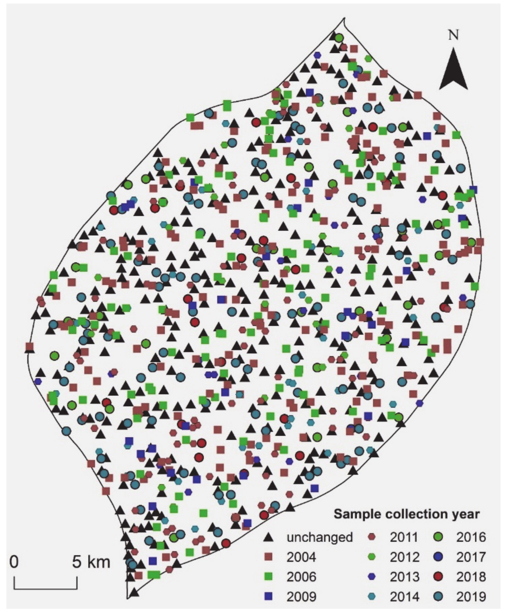
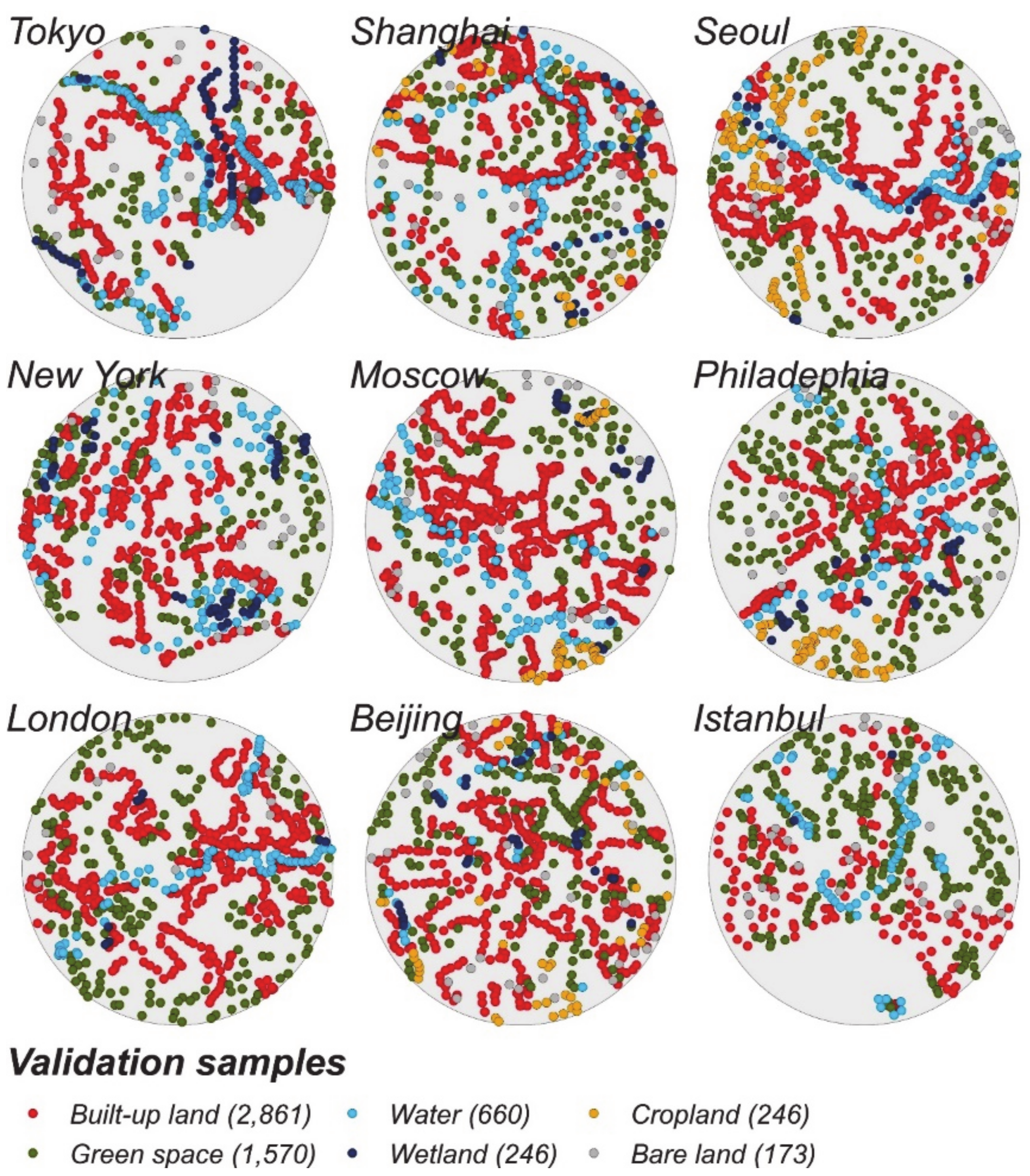
The statistically robust method proposed by [43] was employed to assess the map accuracy. In brief, the accuracy is measured by adjusting with the areal extent of LCLU. Our previous work accumulated 311 unchanged samples that could be used to assess the accuracy [16,17]. In addition, through stratified sampling, we supplemented 677 samples by inspecting Google Earth images with very-high-resolution [24,37]. The accuracy of maps for 2004, 2006, 2009, 2011, 2012, 2013, 2014, 2016, 2017, 2018, and 2019 was assessed because of an insufficient amount of very-high-resolution images. Figure A1 shows the distribution of samples. To test the availability of our methodology, we generated urban LCLU maps of nine big cities in the world for 2019. Correspondingly, we collected 5756 samples from Google Earth for accuracy assessment (Figure A3).

2.5. Land Dynamic Analysis

The abrupt change (or turning-point) detection and change rate computation of LCLUC were conducted. The turning-point of LCLUC during the period considered was obtained by Pettitt’s test, which is a nonparametric method [44]. Specifically, within a continuous observation (e.g., X 1 ,   X 2 ,   ,   X N ), it is supposed that the r i is the rank of data. At each observing place j , the sum of ranks W j could be computed,
W j = i = 1 j r i
where the j is ranged from 1 to N - 1 . Hereafter, the statistic T j was introduced to infer the turning-point.
T j = 2 W j - j N + 1
If the absolute value of the statistic T j reaches its maximum at j = J , then the turning-point occurs in time J [45]. For the turning time J , it is necessary to evident whether the estimation is significant using the sampling distribution of W j . The approximate statistic P was introduced, and the turning estimation has been performed with a significant level of 0.01.
P = 2 exp - 6 W J 2 / N 3 + N 2
Hereafter, the annual change rate (ACR) before and after the turning-point could be computed despite the temporal length might be different [37].
ACR = 1 / t 2 - t 1 × ln Area t 2 / Area t 1 × 100
where the t 1 and t 2 denote the early year and later year, respectively. The Area t 1 and Area t 2 denote the LCLU area in the early year and later year, respectively. The ACR is in % · yr - 1 .

2.6. Quantifying Cause and Effect of Land Dynamics

Time-series observations were applied to quantify the drivers and effects of land dynamic by computing correlations between LCLUC, socio-economic statistics, and climate records. The annual socio-economic statistics were collected from the statistic yearbook of Changchun, including urban population (UP), gross domestic product (GDP), GDP of agriculture sector (AS), GDP of industry sector (IS), and GDP of service sector (SS). The climate records of average temperature (ATEM) and average wind velocity (AWV) were collected from the urban station No.54161 of national meteorology (125.2 E, 43.9 N). Further, we quantified the relationship between land dynamic, finer particles (PM2.5), and net primary production (NPP) to learn the effects of LCLUC. Because of lacking continuous PM2.5 data for 2000–2019, we merged the raster dataset from 2000 to 2013 published by [46] and the official annual number from 2014 to 2019. The PM2.5 raster dataset (0.01° resolution) was used to compute the annual mean value within the study area. The product MOD13A3HGF (500-m resolution) was used to compute the annual mean value of NPP within the study area. Thus, the annual change of PM2.5 in 2000–2013 and NPP in 2000–2019 was the mean value of Changchun that was computed based on published products.
We computed the built-up ratio (BR), cropland ratio (CR), green ratio (GR), and green space/built-up ratio (GBR) to echo the previous findings that suggested that green space, built-up area, and cropland changed dominantly in Changchun [8,30,31,35],
BR = pixel built - up / pixel total
CR = pixel cropland / pixel total
GR = pixel green   space / pixel total
GBR = pixel green   space / pixel built - up
where pixel built - up , pixel cropland , pixel green   space , and pixel total denote the pixel area of built-up land, cropland, green space, and Changchun, respectively. Pearson analysis was applied to quantify the correlation coefficients between the observing variables mentioned above for analyzing the driver and effects of LCLUC [9],
r = n × x i y i - x i y i n × x i 2 - x i 2 n × y i 2 - y i 2
where r is the Pearson correlation coefficient. A higher absolute value of r could infer a closer relationship between n pairs of variables x i and y i .

3. Results

3.1. Accuray Report of Annual Maps

The annual LCLU maps of Changchun from 2000 to 2019 were generated with a 15-m resolution. The accuracy assessment reported high overall accuracy (from 0.92 ± 0.03 to 0.98 ± 0.02) of maps (Table 3). Fewer omission errors were reflected by the producer’s accuracy, indicating that our maps agreed with the ground truth. Especially, the user’s accuracy of green space (≥0.84 ± 0.06) and built-up land (≥0.96 ± 0.03) had a slight commission error, laying a good foundation for observing green space and gray space. The bare land showed low accuracy, owing to the spectral similarity of bare ground, built-up area, and sparsely vegetated land. In addition, due to differences in cloud coverage, the yearly brightness image was constructed based on raw images of different numbers. Thus, the default threshold for extracting bare land might change, affecting mapping results (Figure 3). Nonetheless, we temporally neglected that issue to ensure the entire automatic process because the bare land area was few [31,35]. Moreover, good overall accuracy was encouraging the further application of these maps.

3.2. Land Dynamics in Changchun during 2000–2019

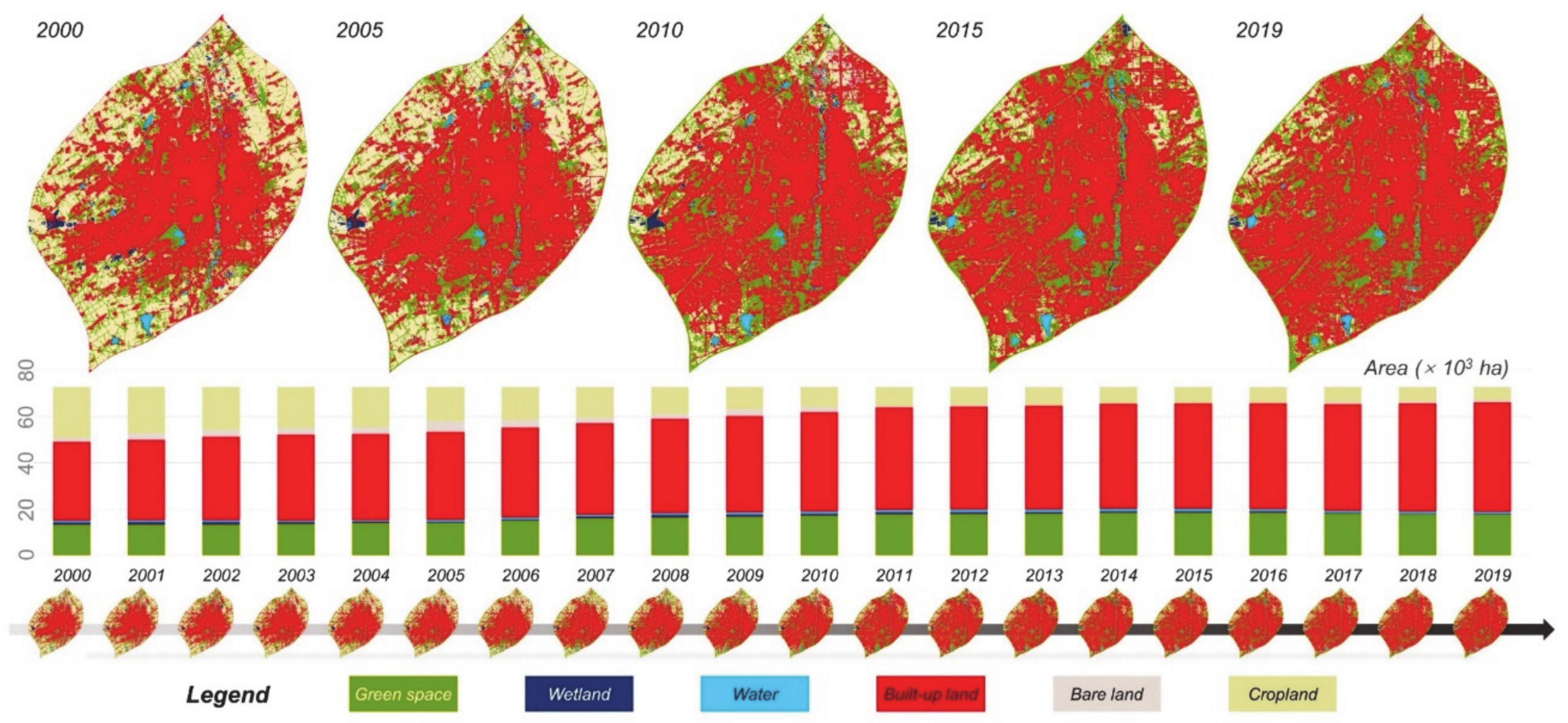
The annual LCLUC of Changchun during 2000-2019 was recorded (Figure 5). The built-up land expansion with the disappearance of cropland was obvious during 2000–2010. The green space exhibited a trend of descent-after-increase, turning at roughly 2011–2016. By contrast, the changes of bare land, water, and wetland were slight, altogether occupying a slight proportion.
The built-up land has been filling the urban space with an annular expansion (Figure 5 and Figure A2). Specifically, the built-up land expanded continually from 34.0 × 10³ ha to 47.5 × 10³ ha, especially before the turning year 2009 (Table 4). The ACR of built-up land from 2000–2009 to 2009–2019 almost halved from 2.24 % · yr - 1 to 1.30 % · yr - 1 , indicating urbanization transitioned from rapid to slow [8]. The cropland lost dramatically from 22.0 × 10³ ha to 5.7 × 10³ ha during 2000–2019. The cropland was encroached upon by the annular expansion of built-up area (Figure A2) [35]. The turning of cropland loss occurred in 2009 as well, and the ACR halved from −9.19 % · yr - 1 to −5.29 % · yr - 1 . Such an observation is in line with the previous study, which suggested the trend of urbanization encroaching on agriculture continually slowed since 2009 [19]. The growth of green space continued from 2000 to 2019 and shifted from rapid (2.66 % · yr - 1 ) to stable (0.43 % · yr - 1 ) in 2009. Though both the built-up land and green space were expanding, their obvious difference in ACR changes deserves in-depth study (Figure A2). Other LCLU exhibited a slight proportion and areal changes. The bare land transitioned from gain to vanishing concurrently with the shifting of rapid-to-slow in built-up expansion. In addition, the water area kept expanding while the wetland kept losing.

3.3. Quantified Correlation of Land Dynamics, Socio-Economic Development, and Environment Change

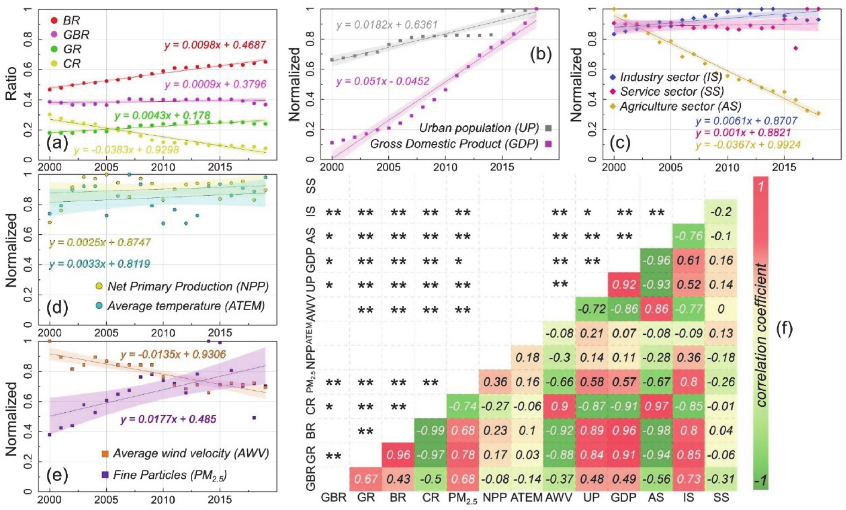
Correlation computation indicated that though the built-up land was filling the urban space; the green space/built-up ratio stayed at ~0.4 (Figure 6a), which related to the areal growth of green space (0.67) (Figure 6f). Regarding socio-economic development, Changchun’s population generally kept increasing (especially after 2014), and GDP grew linearly (Figure 6b). Correspondingly, the land dynamic was significantly driven by immigration and economic process (Figure 6f). The increments of GDP (0.96) primarily encouraged built-up growth, which affirms previous knowledge [9,30], followed by migration (0.89) and industrial progress (0.8). On the other hand, the disappearance of cropland was negatively correlated with the economic and demographic changes, leading to the diving of agricultural production (0.97). The GBR was significantly related to IS (0.73), AS (−0.56), GDP (0.49), and UP (0.48), suggesting GBR was stabilized by industrial development, agricultural contraction, economic progress, and habitat growth.
The urban environment changed over time. The NPP and ATEM changed complicatedly with general trends parallel mutually (Figure 6d). By contrast, the declining trend and increasing trend appeared in the AWV and PM2.5, respectively (Figure 6e). Pearson correlation indicated a close relationship between the AWV, PM2.5, and land dynamics (Figure 6f). Specifically, the AWV negatively related to BR (−0.92) and GR (−0.88), indicating built-up expansion and green space increment decelerated the urban wind. In addition, the PM2.5 was positively related to GR, BR, and GBR, indicating that urban greening and constructing built-up land aggravated air pollution. Such a result deserves in-depth discussion because urban green space could offset emissions and improve air quality, which has been scientifically navigating the urban planning and greening in China during decades [8,17].

4. Discussion

4.1. Availability of Recording Urban Land Dynamics by Integrating Landsat, MDR, and GEE

This study, to our knowledge, has accomplished the first record of urban land dynamics at 15-m resolution, attributing to GEE, Landsat, and MDR algorithm. Currently, GEE is the prevalent tool to observe LCLUC for global to local scale studies [6,11,23]. Large-scale LCLU data, as an important input for modeling and simulating, are furthering the understanding of global change and urban ecology. On the other hand, continuous LCLU data are helping to discover the real process of urban LCLU to correct past concepts derived from time-slice observations (e.g., impervious would not vanish). Especially, high spatiotemporal LCLU data could find the key causes of urban issues that were previously hidden by time-slice mapping [15].
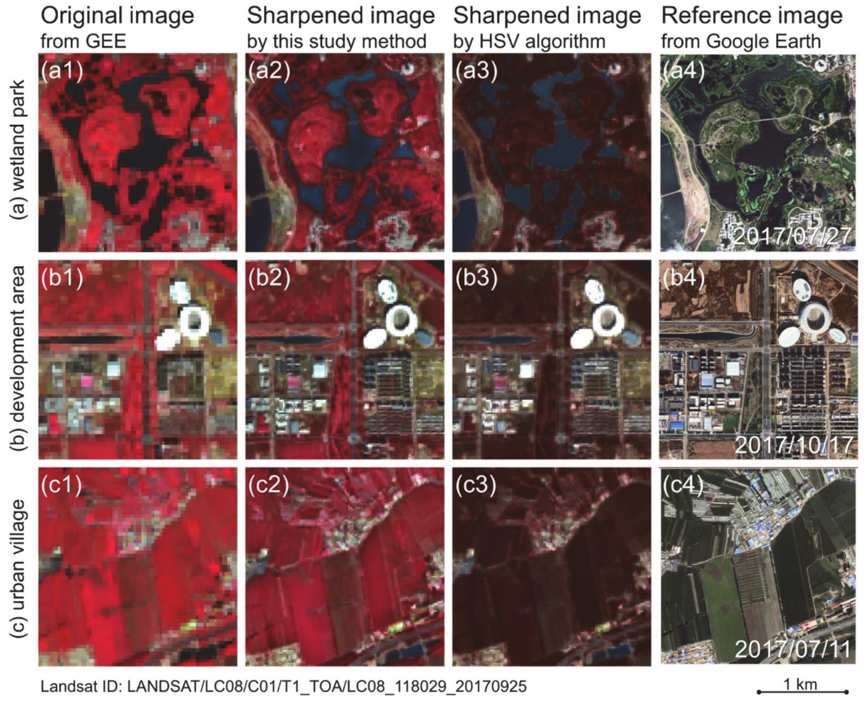
Landsat-based urban mapping was promoted by GEE and MDR. First, GEE’s supercomputing saved time taken in downloading, preprocessing, mosaic, etc. [17]. Second, multispectral bands were fully applied to construct spectral indices or rule nodes that could extract urban LCLU [13,24,36]. This study exactly utilized the urban phenology and ecology to generate annual maps with good accuracy (Table 2), indicating MDR is an effective classifier for mapping urban LCLU. What is more, compared with the built-in algorithm of GEE (i.e., HSV method), our pan-sharpening method saved the original multispectral information of Landsat while also enhancing the image resolution (Figure 7). Although HSV could enhance pixel heterogeneity, it changed the original spectral information. Therefore, our method could be an alternative to HSV for the dual goals of saving spectral information and enhancing image resolution. Our pan-sharpening method implies a question: To what extent can 15-m LCLU maps enhance the overall accuracy from 30-m maps? Given that 30-m pixel concealed real land cover, it is expected that 15-m maps could promote mapping accuracy [21,27]. Moreover, we applied the 5 × 5 pixel-window to avoid the loss of spectral information (Figure 2), whether other window-size could help pixel unmixing is an interesting question.
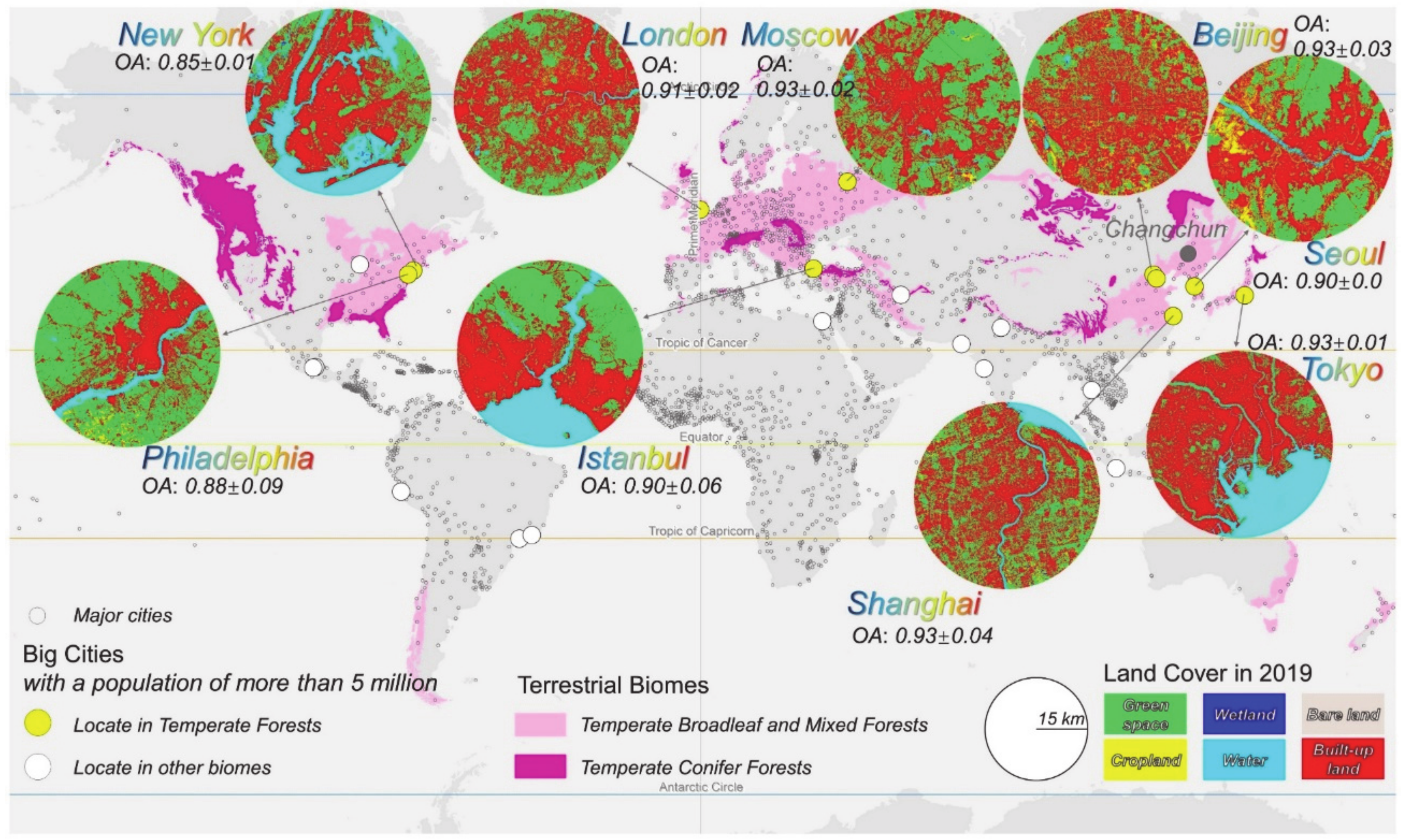
It is available and replicable to map LCLU of other cities by our methodology. For testing the availability of our methodology, we mapped the urban LCLU for nine big cities that share the same biomes with Changchun and have a population of more than five million (Figure 8). Within a 15 km radius, the urban LCLU can be mapped with high accuracy (0.85 ± 0.01 to 0.93 ± 0.01) (Figure 8). Thus, under the condition of temperate biomes, our method could be applied to map urban LCLU at 15-m resolution. Differentiating vegetation could be a difficult step because forest, grass, and crops exhibit similar spectral information during the growing season. However, non-vegetation land could be directly extracted by adjusting shortwave infrared bands or other spectral indices [36,37,38]. In this study, the non-vegetation mapping part that considered spectral variation and cooling-island could be directly used to map similar LCLU categories (Figure 3). Previous studies employed machine learning classifiers to map different vegetation through “black box” that learn knowledge from spectral indices [14,47]. The difference of this study is that the phenology of green space and cropland was well analyzed (Figure 4), implying the necessity of our method is the difference of growth time between different vegetation land covers.
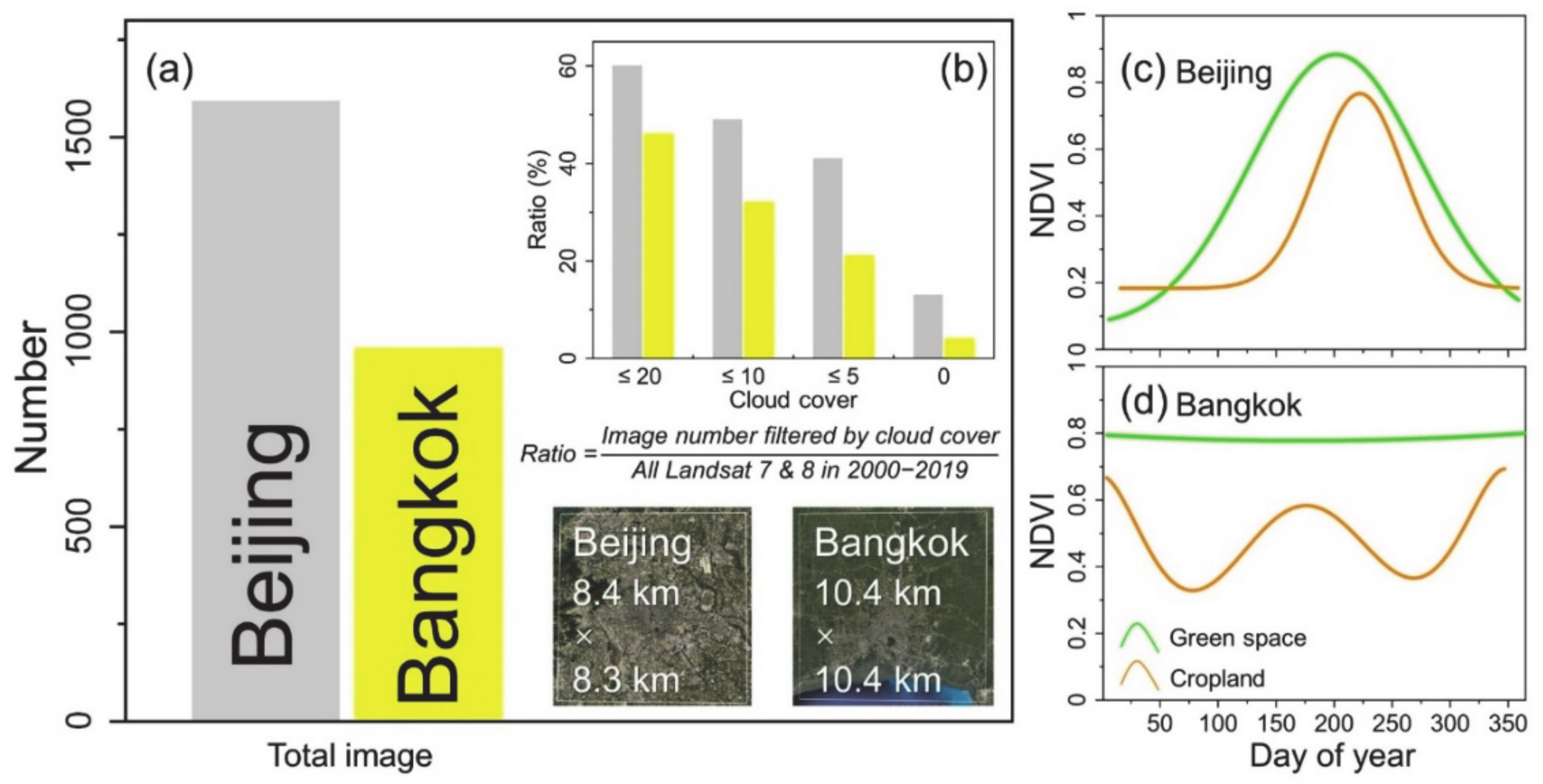
However, by our test, our method is currently not suitable for southern cities because of a lack of clean images and fewer phenology differences between the green space and crops. For example, in the past two decades, the total number of ETM+ and OLI images in Bangkok is 959, while the number of Beijing is 1593 (Figure 9a). For Beijing, the cloud cover in 60% of the images is less than or equal to 20%, and the phenology of green space and cropland in Beijing is distinct, laying a good foundation for mapping by the MDR method (Figure 9a). By contrast, for Bangkok, the ratio of low cloud cover images is smaller (Figure 9b). Especially, warmer climates make double-cropping possible in southern cities (Figure 9c), which reduced the chance of mapping forest and cropland directly based on the NDVI threshold (Figure 3). In addition, the similar structure of tall crops (e.g., oil palm) and forest in Southern countries makes their differentiation difficult [48]. Future work can start with building composite indices, thresholding by phenology fluctuation, adding texture information, or fitting image gaps to improve Southern urban LCLU mapping [6,41].

4.2. Time-Series Land Dynamic for Understanding Urbanization in Changchun

Changchun’s 21st century exhibited characteristics of industrialization and de-agrarianization with the expansion of built-up land and the disappearance of cropland (Figure 5). Previous studies reported a similar urbanization trend of Changchun by time-slice observation of the 2000s [30,31,35], but this study qualified the turning point of LCLU through continuous data of the entire 2000s–2010s. The year 2009 was the transition of Changchun as the ACR of major LCLU halved (Table 3), which could be the epitome of China’s land use transformation from agriculture to city [19]. The temporal cost of China’s urbanization reduced in the 2000s [49]. Therefore, it is necessary to ascertain what land transformed into new urban area and its effects after 2009 when the “red line” national policy proposed to maintain a basic area of cropland.
The overall economic progress promoted the growth of the BR and GR and the loss of CR, and the urban population growth and industrial production played a major role (Figure 6). However, it is doubtful that the sustainable development in Changchun could achieve under those relationships. First, the industry-driven economy has faded in Northeast China and Jilin province in recent years [34], slowing down the expansion of built-up areas. This is a reasonable observation because the economic depression discourages investment, the emergence of high-tech industry, and the attraction of talent. The housing bubble in the early years has gradually disappeared, which could further deteriorate the economy. In addition, the administrative policy has become the major driver of urban development as the gradually decoupling between population, economy, and impervious in China [9]. In 2008, the National Eco-functional Zoning announced that the primary task of Northeast China was grain production and environment protection, which could further limit the industrial and urban development in Changchun. Though we neglected the urban volume increment as Landsat observations only reflect two-dimensional land changes, the second-rate positioning has destined the depressing economy and misty urban future in the short-term.

4.3. Implication from Building the City of Garden in Changchun

As the only northern one of four Garden Cities, Changchun has been working hard to make the urban environment more aesthetic, habitable, and famous. In 20 years, the GBR of ~0.4 indicated that Changchun did well in greening under the urbanization (Figure 6a). This was partly because industrial production caused air pollution and urged more green space to promote air quality, which was inferred by a significant relationship between the IS, PM2.5, and GR (Figure 6f). Nonetheless, though green space could mitigate emissions [17], the increasing GR significantly related to anabatic PM2.5 (Figure 6). This relationship deserves serious consideration because the national policy New-type Urbanization Plan published in 2014 has been asking cities to construct more green space to enhance the urban environment.
The increase in PM2.5 was significantly related to the AWV descent (Figure 6f). Though our study showed that impervious expansion was slowing down in recent years (Figure 5), the BR was significantly related to AWV descent (Figure 6f). The situation might be because of building density increasing by transforming inefficient land (e.g., urban villages) to economically efficient land (e.g., office building) under the old city renovation project in China. However, like what was observed for BR, the increasing GR significantly declined wind speed (Figure 6). In other words, filling green space could likely hinder the airflow and thus centralize finer particles. This finding may be limited by the resolution of the PM2.5 raster and the effectiveness of the official public data, which needs verification by integrating LCLU maps and finer PM2.5 raster. By this study, the purposive thinning of forest density might be an effective way to strengthen the air exchange and air quality suggested by the concurrent descent of PM2.5 and GBR after 2015 (Figure 6a,e).

5. Conclusions

We presented an approach to map annual urban LCLUC at high resolution (15-m) with Landsat images using GEE. With this method, we could capture the LCLUC in Changchun, and analyze the social-economic drivers and environmental effects of LCLUC. The continued urban expansion, green space growth, and cropland loss characterized LCLUC in Changchun. The LCLUC was primarily driven by economic development, immigration, and industrialization. However, inevitable urbanization under the environment of national economic development and ecological protection would weaken the sustainability of the urban development. With China’s emphasis on economic development and ecosystem conservation such as the Belt and Road initiative, urban planners should explore strategies for urban sustainable development.
New knowledge about urban LCLUC in Changchun was revealed through our study. The year 2009 was the turning point of land dynamics from high-frequency to low-frequency in Changchun. The growth of built-up land and green space hindered airflow and thus increased PM2.5. Our research enhances the understanding of the impacts of urbanization on the environment. As air pollution has been one of the main concerns of the Chinese government, controlling air pollution and urban sustainable management requires research across different scales from local to national.

Author Contributions

Conceptualization, Y.D. and Z.R.; methodology, Y.D.; software, Y.D. and Y.F.; validation, Y.F., Z.M., and R.Y.; formal analysis, Y.D., Y.S., and Y.F.; data curation, Z.R.; writing—original draft preparation, Y.D.; writing—review and editing, Z.R.; visualization, Y.D.; supervision, X.H.; project administration, X.H. and Z.R.; funding acquisition, X.H. and Z.R. All authors have read and agreed to the published version of the manuscript.

Funding

This work was funded in part by the Youth Science Fund Project approved by the Youth Innovation Promotion Association of Chinese Academy of Sciences under Grant 2020237, in part by the National Natural Science Foundation of China under Grant 41701210, in part by the Science Development Project of Jilin province under Grant 20190303067SF, and in part by the Project of Jilin Province Water Resources Department under Grant 12600220190012.

Acknowledgments

The authors would like to thank Qiuyan Yu from New Mexico State University for constructive comments and suggestions. The authors would like to thank the four anonymous reviewers and the assigned editor for constructive comments and suggestions. The authors would like to thank the book Advances in Geosciences volume 16 (online edition) for the illustration of Pettitt’s Test. The authors would like to thank net friends from the website gis.stackexchange.com for generously professional instruction of GEE operation.

Conflicts of Interest

The authors declare no conflict of interest.

Appendix A

Figure A1. Distribution of samples applied for accuracy assessment.
Remotesensing 12 02451 g0a1
Figure A2. Maps showing the annual change rate of three major land cover types from 2000 to 2019. For demonstration purposes, the spatial statistical process was conducted in a pixel of 1.5 km × 1.5 km because the original pixel length is 15-m. ACR: annual change rate.
Remotesensing 12 02451 g0a2
Figure A3. Distribution of validation samples used for assessing the accuracy of big city maps. These samples were collected by stratified sampling from Google Earth. See Figure 8 for the maps.
Remotesensing 12 02451 g0a3

References

  1. Grimm, N.B.; Faeth, S.H.; Golubiewski, N.E.; Redman, C.L.; Wu, J.; Bai, X.; Briggs, J.M. Global change and the ecology of cities. Science 2008, 319, 756–760. [Google Scholar] [CrossRef] [PubMed] [Green Version]
  2. UN. World Urbanization Prospects: The 2018 Revision (ST/ESA/SER.A/420); United Nations: New York, NY, USA, 2019. [Google Scholar]
  3. Seto, K.C.; Ramankutty, N. Hidden linkages between urbanization and food systems. Science 2016, 352, 943–945. [Google Scholar] [CrossRef] [PubMed]
  4. Angel, S.; Parent, J.; Civco, D.L.; Blei, A.; Potere, D. The dimensions of global urban expansion: Estimates and projections for all countries, 2000–2050. Prog. Plann. 2011, 75, 53–107. [Google Scholar] [CrossRef]
  5. Rockstrom, J.; Steffen, W.; Noone, K.; Persson, A.; Chapin, F.S., III; Lambin, E.F.; Lenton, T.M.; Scheffer, M.; Folke, C.; Schellnhuber, H.J.; et al. A safe operating space for humanity. Nature 2009, 461, 472–475. [Google Scholar] [CrossRef] [PubMed]
  6. Liu, X.; Huang, Y.; Xu, X.; Li, X.; Li, X.; Ciais, P.; Lin, P.; Gong, K.; Ziegler, A.D.; Chen, A.; et al. High-spatiotemporal-resolution mapping of global urban change from 1985 to 2015. Nat. Sustain. 2020. [Google Scholar] [CrossRef]
  7. Van Vliet, J. Direct and indirect loss of natural area from urban expansion. Nat. Sustain. 2019, 2, 755–763. [Google Scholar] [CrossRef]
  8. Dou, Y.Y.; Kuang, W.H. A comparative analysis of urban impervious surface and green space and their dynamics among 318 different size cities in China in the past 25 years. Sci. Total Environ. 2020, 706, 135828. [Google Scholar] [CrossRef]
  9. Kuang, W. National urban land-use/cover change since the beginning of the 21st century and its policy implications in China. Land Use Policy 2020, 97, 104747. [Google Scholar] [CrossRef]
  10. Kuang, W.; Chi, W.; Lu, D.; Dou, Y. A comparative analysis of megacity expansions in China and the U.S.: Patterns, rates and driving forces. Landsc. Urban Plan. 2014, 132, 121–135. [Google Scholar] [CrossRef]
  11. Gong, P.; Li, X.; Wang, J.; Bai, Y.; Cheng, B.; Hu, T.; Liu, X.; Xu, B.; Yang, J.; Zhang, W.; et al. Annual maps of global artificial impervious area (GAIA) between 1985 and 2018. Remote Sens. Environ. 2020, 236, 111510. [Google Scholar] [CrossRef]
  12. Phiri, D.; Morgenroth, J. Developments in Landsat Land Cover Classification Methods: A Review. Remote Sens. 2017, 9, 967. [Google Scholar] [CrossRef] [Green Version]
  13. Zhong, Q.; Ma, J.; Zhao, B.; Wang, X.; Zong, J.; Xiao, X. Assessing spatial-temporal dynamics of urban expansion, vegetation greenness and photosynthesis in megacity Shanghai, China during 2000–2016. Remote Sens. Environ. 2019, 233, 111374. [Google Scholar] [CrossRef]
  14. Zhao, Y.; Feng, D.; Yu, L.; Cheng, Y.; Zhang, M.; Liu, X.; Xu, Y.; Fang, L.; Zhu, Z.; Gong, P. Long-Term Land Cover Dynamics (1986–2016) of Northeast China Derived from a Multi-Temporal Landsat Archive. Remote Sens. 2019, 11, 599. [Google Scholar] [CrossRef] [Green Version]
  15. Reba, M.; Seto, K.C. A systematic review and assessment of algorithms to detect, characterize, and monitor urban land change. Remote Sens. Environ. 2020, 242, 111739. [Google Scholar] [CrossRef]
  16. Ren, Z.; He, X.; Zheng, H.; Zhang, D.; Yu, X.; Shen, G.; Guo, R. Estimation of the Relationship between Urban Park Characteristics and Park Cool Island Intensity by Remote Sensing Data and Field Measurement. Forests 2013, 4, 868–886. [Google Scholar] [CrossRef] [Green Version]
  17. Ren, Z.; Zheng, H.; He, X.; Zhang, D.; Shen, G.; Zhai, C. Changes in spatio-temporal patterns of urban forest and its above-ground carbon storage: Implication for urban CO2 emissions mitigation under China’s rapid urban expansion and greening. Environ. Int. 2019, 129, 438–450. [Google Scholar] [CrossRef]
  18. Fang, D.; Wang, Q.; Li, H.; Yu, Y.; Lu, Y.; Qian, X. Mortality effects assessment of ambient PM2.5 pollution in the 74 leading cities of China. Sci. Total Environ. 2016, 569, 1545–1552. [Google Scholar] [CrossRef]
  19. Qiu, B.; Li, H.; Tang, Z.; Chen, C.; Berry, J. How cropland losses shaped by unbalanced urbanization process? Land Use Policy 2020, 96, 104715. [Google Scholar] [CrossRef]
  20. He, C.; Liu, Z.; Xu, M.; Ma, Q.; Dou, Y. Urban expansion brought stress to food security in China: Evidence from decreased cropland net primary productivity. Sci. Total Environ. 2017, 576, 660–670. [Google Scholar] [CrossRef]
  21. Zhou, W.Q.; Wang, J.; Qian, Y.G.; Pickett, S.T.A.; Li, W.F.; Han, L.J. The rapid but "invisible" changes in urban greenspace: A comparative study of nine Chinese cities. Sci. Total Environ. 2018, 627, 1572–1584. [Google Scholar] [CrossRef]
  22. Gorelick, N.; Hancher, M.; Dixon, M.; Ilyushchenko, S.; Thau, D.; Moore, R. Google Earth Engine: Planetary-scale geospatial analysis for everyone. Remote Sens. Environ. 2017, 202, 18–27. [Google Scholar] [CrossRef]
  23. Donchyts, G.; Baart, F.; Winsemius, H.; Gorelick, N.; Kwadijk, J.; van de Giesen, N. Earth’s surface water change over the past 30 years. Nat. Clim. Chang. 2016, 6, 810–813. [Google Scholar] [CrossRef]
  24. Dong, J.; Xiao, X.; Menarguez, M.A.; Zhang, G.; Qin, Y.; Thau, D.; Biradar, C.; Moore, B., III. Mapping paddy rice planting area in northeastern Asia with Landsat 8 images, phenology-based algorithm and Google Earth Engine. Remote Sens. Environ. 2016, 185, 142–154. [Google Scholar] [CrossRef] [PubMed] [Green Version]
  25. Gong, P.; Liu, H.; Zhang, M.; Li, C.; Wang, J.; Huang, H.; Clinton, N.; Ji, L.; Li, W.; Bai, Y.; et al. Stable classification with limited sample: Transferring a 30-m resolution sample set collected in 2015 to mapping 10-m resolution global land cover in 2017. Sci. Bull. 2019, 64, 370–373. [Google Scholar] [CrossRef] [Green Version]
  26. Pan, T.; Kuang, W.; Hamdi, R.; Zhang, C.; Zhang, S.; Li, Z.; Chen, X. City-Level Comparison of Urban Land-Cover Configurations from 2000-2015 across 65 Countries within the Global Belt and Road. Remote Sens. 2019, 11, 1515. [Google Scholar] [CrossRef] [Green Version]
  27. Gilbertson, J.K.; Kemp, J.; van Niekerk, A. Effect of pan-sharpening multi-temporal Landsat 8 imagery for crop type differentiation using different classification techniques. Comput. Electron. Agric. 2017, 134, 151–159. [Google Scholar] [CrossRef] [Green Version]
  28. Meng, X.; Shen, H.; Li, H.; Zhang, L.; Fu, R. Review of the pansharpening methods for remote sensing images based on the idea of meta-analysis: Practical discussion and challenges. Inf. Fusion 2019, 46, 102–113. [Google Scholar] [CrossRef]
  29. Google. Spectral Transformations. Available online: https://developers.google.com/earth-engine/image_transforms (accessed on 21 May 2020).
  30. Chen, L.; Ren, C.; Zhang, B.; Wang, Z.; Liu, M. Quantifying Urban Land Sprawl and its Driving Forces in Northeast China from 1990 to 2015. Sustainability 2018, 10, 188. [Google Scholar] [CrossRef] [Green Version]
  31. Kuang, W.; Yan, F. Urban structural evolution over a century in Changchun city, Northeast China. J. Geogr. Sci. 2018, 28, 1877–1895. [Google Scholar]
  32. Li, G.Y.; Li, L.W.; Lu, D.S.; Guo, W.; Kuang, W.H. Mapping impervious surface distribution in China using multi-source remotely sensed data. GISci. Remote Sens. 2020, 57, 543–552. [Google Scholar] [CrossRef]
  33. Roy, D.P.; Kovalskyy, V.; Zhang, H.K.; Vermote, E.F.; Yan, L.; Kumar, S.S.; Egorov, A. Characterization of Landsat-7 to Landsat-8 reflective wavelength and normalized difference vegetation index continuity. Remote Sens. Environ. 2016, 185, 57–70. [Google Scholar] [CrossRef] [PubMed] [Green Version]
  34. Mao, D.; He, X.; Wang, Z.; Tian, Y.; Xiang, H.; Yu, H.; Man, W.; Jia, M.; Ren, C.; Zheng, H. Diverse policies leading to contrasting impacts on land cover and ecosystem services in Northeast China. J. Clean. Prod. 2019, 240, 117961. [Google Scholar] [CrossRef]
  35. Sun, Y.; Zhao, S.; Qu, W. Quantifying spatiotemporal patterns of urban expansion in three capital cities in Northeast China over the past three decades using satellite data sets. Environ. Earth Sci. 2015, 73, 7221–7235. [Google Scholar] [CrossRef]
  36. Li, X.; Gong, P. An "exclusion-inclusion" framework for extracting human settlements in rapidly developing regions of China from Landsat images. Remote Sens. Environ. 2016, 186, 286–296. [Google Scholar] [CrossRef]
  37. Dong, Y.; Ren, Z.; Wang, Z.; Yu, Q.; Zhu, L.; Yu, H.; Bao, G. Spatiotemporal Patterns of Forest Changes in Korean Peninsula Using Landsat Images During 1990–2015: A Comparative Study of Two Neighboring Countries. IEEE Access 2020, 8, 73623–73633. [Google Scholar] [CrossRef]
  38. Zhang, L.; Li, X.; Yuan, Q.; Liu, Y. Object-based approach to national land cover mapping using HJ satellite imagery. J. Appl. Remote Sens. 2014, 8, 083686. [Google Scholar] [CrossRef]
  39. Xue, Z.; Hou, G.; Zhang, Z.; Lyu, X.; Jiang, M.; Zou, Y.; Shen, X.; Wang, J.; Liu, X. Quantifying the cooling-effects of urban and peri-urban wetlands using remote sensing data: Case study of cities of Northeast China. Landsc. Urban Plan. 2019, 182, 92–100. [Google Scholar] [CrossRef]
  40. Otsu, N. Threshold Selection Method from Gray-Level Histograms. IEEE Trans. Syst. Man. Cybern. 1979, 9, 62–66. [Google Scholar] [CrossRef] [Green Version]
  41. Venkatappa, M.; Sasaki, N.; Shrestha, R.P.; Tripathi, N.K.; Ma, H.-O. Determination of Vegetation Thresholds for Assessing Land Use and Land Use Changes in Cambodia Using the Google Earth Engine Cloud-Computing Platform. Remote Sens. 2019, 11, 1514. [Google Scholar] [CrossRef] [Green Version]
  42. Li, X.; Zhou, Y.; Asrar, G.R.; Meng, L. Characterizing spatiotemporal dynamics in phenology of urban ecosystems based on Landsat data. Sci. Total Environ. 2017, 605, 721–734. [Google Scholar] [CrossRef]
  43. Olofsson, P.; Foody, G.M.; Herold, M.; Stehman, S.V.; Woodcock, C.E.; Wulder, M.A. Good practices for estimating area and assessing accuracy of land change. Remote Sens. Environ. 2014, 148, 42–57. [Google Scholar] [CrossRef]
  44. Pettitt, A.N. A Non-Parametric Approach to the Change-Point Problem. J. R. Stat. Soc. Ser. C (Appl. Stat.) 1979, 28, 126–135. [Google Scholar] [CrossRef]
  45. Verstraeten, G.; Poesen, J.; Demarée, G.; Salles, C. Long-term (105 years) variability in rain erosivity as derived from 10-min rainfall depth data for Ukkel (Brussels, Belgium): Implications for assessing soil erosion rates. J. Geophys. Res. Atmos. 2006, 111. [Google Scholar] [CrossRef]
  46. Van Donkelaar, A.; Martin, R.V.; Brauer, M.; Hsu, N.C.; Kahn, R.A.; Levy, R.C.; Lyapustin, A.; Sayer, A.M.; Winker, D.M. Global Estimates of Fine Particulate Matter using a Combined Geophysical-Statistical Method with Information from Satellites, Models, and Monitors. Environ. Sci. Technol. 2016, 50, 3762–3772. [Google Scholar] [CrossRef]
  47. Maxwell, A.E.; Warner, T.A.; Fang, F. Implementation of machine-learning classification in remote sensing: An applied review. Int. J. Remote Sens. 2018, 39, 2784–2817. [Google Scholar] [CrossRef] [Green Version]
  48. Tropek, R.; Sedlacek, O.; Beck, J.; Keil, P.; Musilova, Z.; Simova, I.; Storch, D. Comment on “High-resolution global maps of 21st-century forest cover change”. Science 2014, 344. [Google Scholar] [CrossRef] [Green Version]
  49. Zhao, S.; Zhou, D.; Zhu, C.; Sun, Y.; Wu, W.; Liu, S. Spatial and Temporal Dimensions of Urban Expansion in China. Environ. Sci. Technol. 2015, 49, 9600–9609. [Google Scholar] [CrossRef]
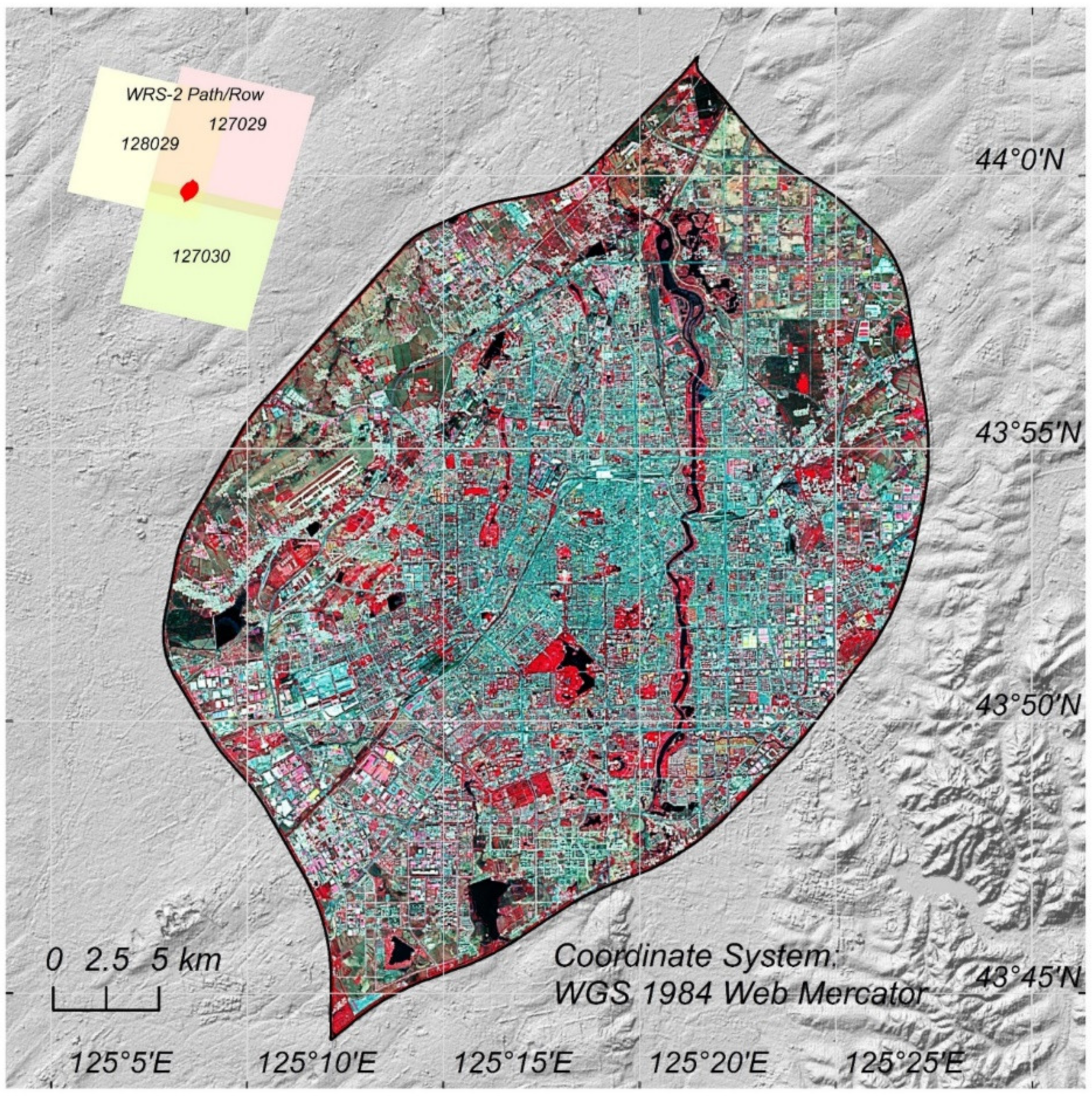
Figure 1. Location of Changchun city defined by the outermost highway ring. The WRS-2 path/row shows three Landsat scenes that occupy the study area.
Remotesensing 12 02451 g001
Figure 2. Correlation of the original band values and their pan-sharpened counterparts. This study pan-sharpened Landsat images by a 5 × 5 pixel-window that reserves the spectral information and enhances the spatial heterogeneity of pixels.
Remotesensing 12 02451 g002
Figure 3. Integrated processing of automatic thresholding and multilevel decision rule. DOY: day of year.
Remotesensing 12 02451 g003
Figure 4. NDVI fluctuations show the phenological difference between green space and cropland in Changchun. (a) Fitted NDVI indicates the earlier growth of green space. (b) Land surface temperature dynamics indicate crops start to ripen after DOY 208 due to an accumulation of daytime temperature of more than 1900 Celsius. (c) Derivative of fitted NDVI. SOS: start of season; SOP: start of peak; EOP: end of peak, EOS: end of season. See [42] for remotely sensed urban phenology.
Remotesensing 12 02451 g004
Figure 5. Annual distribution and areal extent of land cover land use in Changchun from 2000 to 2019. Raster maps of the year 2000, 2005, 2010, 2015, and 2019 are zoomed in for a demo purpose.
Remotesensing 12 02451 g005
Figure 6. Statistical relationships between land dynamics, socio-economic records, and environmental fluctuation. Panels (ae) are normalized changes in observing variables. Note that the single star (*) and double star (**) indicate statistical significance at 0.05 and 0.01, respectively. BR: built-up ratio; GBR: green space/built-up ratio; GR: green ratio; CR: cropland ratio; UP: urban population; GDP: gross domestic product; AS: GDP of agriculture sector; IS: GDP of industry sector; SS: GDP of service sector; NPP: net primary production; ATEM: average temperature; AWV: average wind velocity; PM2.5: fine particles.
Remotesensing 12 02451 g006
Figure 7. Inter-comparison of the original Landsat 8 image and its pan-sharpened counterparts by different methods. Panels (ac) are examples of different locations. The HSV algorithm is a built-in method in GEE [29]. The Landsat ID indicates that the compared image is a TOA image of the OLI sensor derived from 25 September 2017, and its path/row is 118/29.
Remotesensing 12 02451 g007
Figure 8. Test results show the availability of this study method in mapping urban land cover land use for temperate cities. For a demo purpose, only cities with a population of more than 5 million have considered. OA: overall accuracy. See Figure A3 for the distribution of validation samples.
Remotesensing 12 02451 g008
Figure 9. The total number of Landsat images from 2000 to 2019 indicates a less clean observation for Bangkok than that for Beijing. (a) Within the areal extent of 8.4 km × 8.3 km in Beijing and 10.4 km × 10.4 km in Bangkok, respectively, the total image number of Landsat 7 and Landsat 8 from 2000 to 2019. (b) Number ratio of images filtered by cloud cover. Panels (c,d) are the phenology of Beijing and Bangkok, respectively.
Remotesensing 12 02451 g009
Table 1. Brief information about applied Landsat TOA in GEE environment.
SensorPeriodBandAnnual CompositePanchromatic Source
TM2000–2012G, R, NIR, SWIR1, SWIR2, LSTYesNo
ETM+2000–2019G, R, NIR, SWIR1, SWIR2, LST, PanYesYes
OLI2013–2019YesYes
Note: G: green, R: red; NIR: near-infrared, SWIR1: short-wave infrared 1; SWIR2: short-wave infrared 2; LST: land surface temperature; Pan: panchromatic.
Table 2. Definition of urban land cover land use category in this study.
CodeCategoryBrief Description
10Green spaceNatural or artificial vegetated land includes forest, shrub, grass, etc.
20WetlandWater environment in which herbs seasonally grows.
30WaterNatural or artificial lake, channel, pond, etc.
40Built-up landArtificial infrastructure for living, transport, production, etc.
50Bare landAbandoned, cleared, or in-planning urban space.
60CroplandRegular shaped arable land for grain growing.
Table 3. Report of map accuracy.
ItemYear
20042006200920112012201320142016201720182019
GSPA0.82 ± 0.060.86 ± 0.060.94 ± 0.050.99 ± 0.030.94 ± 0.060.94 ± 0.060.9 ± 0.030.96 ± 0.040.93 ± 0.030.91 ± 0.020.95 ± 0.03
UA0.86 ± 0.060.91 ± 0.060.92 ± 0.050.98 ± 0.030.85 ± 0.060.84 ± 0.060.97 ± 0.030.93 ± 0.040.95 ± 0.040.98 ± 0.020.97 ± 0.03
WLPA0.63 ± 0.010.78 ± 0.010.96 ± 0.010.79 ± 0.010.91 ± 0.010.9 ± 0.010.86 ± 0.010.89 ± 0.010.84 ± 0.010.86 ± 0.010.9 ± 0.01
UA0.85 ± 0.20.67 ± 0.410.85 ± 0.20.96 ± 0.090.96 ± 0.090.92 ± 0.110.71 ± 0.360.83 ± 0.330.73 ± 0.280.8 ± 0.390.9 ± 0.13
WAPA0.85 ± 0.140.87 ± 0.390.84 ± 0.180.79 ± 0.270.96 ± 0.30.81 ± 0.30.78 ± 0.310.79 ± 0.230.95 ± 0.260.91 ± 0.220.96 ± 0.13
UA0.91 ± 0.120.75 ± 0.320.84 ± 0.150.75 ± 0.220.71 ± 0.250.59 ± 0.240.75 ± 0.260.86 ± 0.190.76 ± 0.210.83 ± 0.180.92 ± 0.11
BTPA0.96 ± 0.040.99 ± 0.060.97 ± 0.030.99 ± 0.030.97 ± 0.020.96 ± 0.020.96 ± 0.020.95 ± 0.020.95 ± 0.030.94 ± 0.010.95 ± 0.02
UA0.97 ± 0.040.96 ± 0.030.98 ± 0.020.98 ± 0.020.99 ± 0.010.99 ± 0.010.99 ± 0.010.98 ± 0.010.98 ± 0.020.99 ± 0.010.99 ± 0.01
BLPA0.8 ± 0.220.74 ± 0.280.83 ± 0.170.38 ± 0.150.61 ± 0.460.59 ± 0.520.3 ± 0.60.17 ± 0.30.52 ± 0.40.93 ± 0.010.68 ± 0.35
UA0.71 ± 0.170.79 ± 0.220.88 ± 0.140.94 ± 0.120.5 ± 0.370.67 ± 0.410.6 ± 0.480.82 ± 0.240.75 ± 0.320.97 ± 0.010.86 ± 0.28
CLPA0.93 ± 0.080.83 ± 0.090.79 ± 0.070.94 ± 0.040.79 ± 0.080.82 ± 0.090.85 ± 0.140.79 ± 0.070.79 ± 0.10.88 ± 0.170.84 ± 0.14
UA0.87 ± 0.080.87 ± 0.090.9 ± 0.070.98 ± 0.040.89 ± 0.080.91 ± 0.090.74 ± 0.140.9 ± 0.070.84 ± 0.10.73 ± 0.170.85 ± 0.14
Overall accuracy0.92 ± 0.030.92 ± 0.040.95 ± 0.030.98 ± 0.020.94 ± 0.020.94 ± 0.020.95 ± 0.020.96 ± 0.020.95 ± 0.020.96 ± 0.020.97 ± 0.02
Note: GS: green space; WT: wetland; WA: water; BT: built-up land; BL: bare land; CL: cropland; UA: user’s accuracy; PA: producer’s accuracy.
Table 4. Turning year of land dynamics.
CategoryTurning ACR   before   Turning   ( % · yr - 1 ) ACR   after   Turning   ( % · yr - 1 )
Green space2009 **2.660.43
Wetland2012−3.39−9.45
Water2009 **1.250.69
Built-up land2009 **2.241.30
Bare land2010 **3.56−10.83
Cropland2009 **−9.19−5.29
Note: the double star (**) indicates statistical significance at 0.01. ACR: annual change rate.