Abstract
We evaluated the performance of three global evapotranspiration (ET) models at local, regional, and global scales using the multiple sets of leaf area index (LAI) and meteorological data from 1982 to 2017 and investigated the uncertainty in ET simulations from the model structure and forcing data. The three ET models were the Simple Terrestrial Hydrosphere model (SiTH) developed by our team, the Priestley–Taylor Jet Propulsion Laboratory model (PT-JPL), and the MODerate Resolution Imaging Spectroradiometer (MODIS) ET algorithm (MOD16). Comparing the observed with simulated monthly ET by the three models over 43 Fluxnet sites, we found that SiTH overestimated ET for forests with mean slope from 1.25 to 1.67, but it performed better than the other two models over short vegetation. MOD16 and PT-JPL models simulated well for forests but poorly in dryland biomes (slope = 0.25~0.55; R2 = 0.02~0.46). At the catchment scale, all models performed well, except for some tropical and high latitudinal catchments, with NSE values lower than 0 and RMSE and MAE values far beyond their mean values. At the global scale, SiTH highly overestimated ET in tropics, while PT-JPL slightly underestimated ET between 30°N and 60°N and MOD16 underestimated ET between 15°S and 30°S. Generally, the PT-JPL provided the better performance than SiTH and MOD16 models. This study also revealed that the estimated ET by SiTH and especially PT-JPL model were influenced by the uncertainty in meteorological data, and the estimated ET was performed better using MERRA-2 datasets for PT-JPL and using ERA5 datasets for SiTH. While the estimated ET by MOD16 were relatively sensitive to LAI data. In addition, our results suggested that the GLOBMAP and GIMMS datasets were more suitable for long-term ET simulations than the GLASS dataset.
1. Introduction
Global terrestrial evapotranspiration (ET) is an important nexus between land surface, vegetation, and atmosphere, and accurately estimating global land ET is of great significance to study global hydrological cycle, energy exchange, carbon cycle, and climate change [1,2,3,4,5]. With the rapid developments in remote sensing, numerous global ET models have been developed in recent decades [6,7,8,9,10,11,12,13,14,15,16,17,18]. In the framework of energy balance theory, the majority of these models use the Penman–Monteith equation (P-M equation) [19] or the Priestley–Taylor approach (P-T approach) [20] to estimate ET. For instance, MOD16, which is the core algorithm of NASA’s MODIS evapotranspiration product, uses the P-M equation to simulate global ET [11]. Fisher et al. [12] proposed a simple, less data-driven, and accurate ET model (PT-JPL) to estimate ET on basis of P-T approach and recently formed the core algorithm of NASA’s ECOSTRESS mission global-scale ET product [13]. In addition, Zhu et al. [18] developed a Simple Terrestrial Hydrosphere model (SiTH) to estimate ET based on the P-T approach and the groundwater–soil–plant–atmosphere continuum (GSPAC) theory. These models have been widely used to study regional or global hydrological cycles [21,22,23,24,25,26,27,28,29].
Despite these progresses in model developments, there are still some insufficiencies in systematic inter-comparisons and evaluations of the model performances. First, there are few systematic assessments of the impact of forcing data uncertainties on global ET model performances [22,30]. As we known, both the vegetation characteristics (leaf area index) and meteorological variables (i.e., radiation, temperature, precipitation, and humidity) may have significant influences on model behaviors. For example, leaf area index (LAI) can influence the amount of absorbed solar radiation and its distributions between plant canopy and soil surface, which ultimately have significant influences on plant transpiration and soil evaporation [31,32,33]. The meteorological conditions regulate the atmospheric evaporation demand and moisture supply, which may have a great influence on ET as the result of global change [2,34]. Over the past 30 years, it has been well documented that there is a constant increase in LAI (Earth greening) [35,36,37], and continuous increasing in land temperature [38]. However, the increasing magnitude and their distributions in different LAI and meteorological datasets were also large [22,36,39]. Thus, it’s urgently needed to systematically evaluate the impacts of the LAI and meteorological forcing data uncertainties on the estimates of ET. Second, the majority of previous studies have focused on evaluating the performances of one specific model over different sites or inter-comparing the performances of different models at single (or a few) locations. For example, Zhang et al. [16] evaluated the performance of the PT-JPL over 44 Fluxnet sites. Ershadi et al. [25] systemtically compared the performances of four ET models over different sites and boimes. To select the best candidate ET model for global applications, it is needed to comprehensively evaluate and intercompare the performances of different models at different spatial scales (local, regional and global) across different biomes and climate conditions. Third, there are still great uncertainties in the long-term changes in ET over the past few decades. For instance, some studies reported that global land ET increased from 1982 to 1998, and then there was a sharp decline until 2008 [2,40,41,42]. Some studies suggested that an upward trend was observed from 1982 to 2000 and an obvious recovery in ET may have started from 2007 [4,43]. Other studies showed that the mean global annual values of terrestrial ET had no significant trend between 2001 and 2018 [44]. To clearly describe the multi-decadal trend in global terrestrial ET, we need to simulate ET using different models with multiple forcing datasets, so that we can properly assess the influences of model structures and forcing data uncertainties on long-term trend of land ET.
In this study, we intercompare the performances of three process-based ET models (MOD16, PT-JPL, and SiTH) at different spatial scales, and obtain a long-term trend of ET based on different combinations of LAI and meteorological datasets. Specifically, the goal of this study is to (i) evaluate the performance of three process-based ET models from local to regional and global scales using different forcing datasets, (ii) analyze the uncertainties due to different model structure and forcing data, and (iii) explore the uncertainty of long-term temporal ET trend in response to climate change and LAI increasing.
2. Methods and Data
2.1. Models Descriptions
2.1.1. SiTH
The SiTH model proposed by Zhu et al. [18] is a relatively new satellite-based ET model at daily temporal resolution. Based on the framework of the groundwater–soil–plant–atmosphere continuum (GSPAC), SiTH uses well-established hydrological models to simulate important hydrological variables (i.e., groundwater, soil moisture, and runoff). Then, the potential evapotranspiration calculated by using P-T equation was constrained down to actual ET through the plant physiological factor and soil moisture conditions. In SiTH, the total ET (mm·day−1) consists of canopy interception evaporation (Ei, mm·day−1), soil evaporation (Es, mm·day−1), and vegetation transpiration (Et, mm·day−1). Soil evaporation is constrained to occur in the first soil layer, while plant transpiration can use both soil water and groundwater. There can be described as:
where fWET is the relative surface wetness (unitless); fSM is the soil moisture constraint (unitless); fT is the constraints of temperature; α is the P-T coefficient (1.26); Δ is the slope of the saturated vapor pressure curve (kPa °C−1); λ is the latent heat of evaporation (MJ·kg−1); γ is the psychrometric constant (0.066 kPa °C−1); Rnc is the net radiation for the canopy (W·m−2) and is given by Rnc = Rn − Rns, where Rn is the net radiation (W·m−2), Rns is the net radiation for surface soil, and G is the soil heat flux (W·m−2); Ts,i is the actual transpiration from the unsaturated soil at the ith layer (i = 1, 2); Tr,g is the actual transpiration from the groundwater; Tp_s,i is the potential transpiration from soil water of the ith layer (mm·day−1); and Tp_g,i is the potential transpiration from groundwater in the ith layer (mm·day−1). The plant physiological and soil moisture constraint functions are calculated as:
where χ is fractional interception occurring during day-time (0.7), Sc (mm·day−1) is the capacity of canopy to store water, Tp (mm·day−1) is the potential transpiration rate of canopy, Ta (°C) is the daily mean air temperature, Topt (°C) is the optimum temperature for canopy transpiration, θi (m3 m−3) is the soil moisture of ith layer, θc,i(m3 m−3) is soil moisture below which plants start to endure water stress for soil layer i, and θwp,i (m3 m−3) is soil moisture at permanent wilting point.
2.1.2. MOD16
The MOD16 model, which was proposed by Mu et al. [10,11], estimated ET based on the P-M equation to calculate potential evaporation [45]. It distributes the available energy into the components of surface soil and vegetation through fractional total vegetation cover. Then, the soil evaporation includes the evaporation from the saturated soil surface and the moist soil surface. Furthermore, canopy water loss includes evaporation from the wet canopy surface and transpiration from the dry surface. Finally, it limits potential ET to actual ET through vegetation physiological factors and meteorological factors. In MOD16, evapotranspiration (E, mm·day−1) is equal to the sum of wet canopy evaporation (Ewet, mm·day−1) and bare soil evaporation (Es, mm·day−1), and vegetation transpiration (ET, mm·day−1) at daytime and nighttime periods. The driving equations in their model are:
where ρ is the air density (kg·m−3), Cp is the specific heat capacity of air (MJ·kg−1·℃−1), ε is the ratio of the molecular weight of water to dry air (i.e., 0.622), Pa is the atmospheric pressure (kPa), VPD is the atmospheric vapor-pressure deficit (kPa), rvc (s·m−1) and rhrc (s·m−1) represent the surface resistance and aerodynamic resistance to evaporated water on the wet canopy surface, respectively, fc is the fractional vegetation cover (dimensionless), rtot (s·m−1) is the total aerodynamic resistance, ras (s·m−1) the aerodynamic resistance at the soil surface, fwet is the relative surface wetness, fsm is the soil water constrain derived from Fisher et al. [12], ra (s·m−1) is the aerodynamic resistance between the mean canopy height and the air above the canopy, and rs (s·m−1) is the canopy surface resistance.
2.1.3. PT-JPL
PT-JPL is a relatively simple (input data and parameters are reduced), accurate model for estimating actual ET at monthly scale [12,25,28,46]. First, PT-JPL estimates potential evapotranspiration based on the P-T equation.Then, plant physiological and ecological constraints (i.e., LAI, green canopy ratio, vegetation temperature, and vegetation moisture) are used to limit potential plant transpiration and atmospheric constraints (vapor pressure deficit and relative humidity) to limit potential soil evaporation to actual ET. PT-JPL divides the actual evapotranspiration (LE, mm·day−1) into three components: canopy transpiration (LEc, mm·day−1), soil evaporation (LEs, mm·day−1), and interception evaporation (LEi, mm·day−1).
where fg is the green canopy fraction (unitless), ft is the plant temperature constraint (unitless), and fm is the plant moisture constraint (unitless). The bio-physiological constraint functions are calculated as:
where the RH is the relative humidity (%), fAPAR is the fraction of photosynthesis active radiation (PAR) absorbed by green vegetation cover, fIPAR is the fraction of PAR intercepted by canopy, Tmax is the air maxium temperature (°C), and β is the sensitivity for fsm to VPD (kPa).
2.2. Input Data
The input data of the above three models includes leaf area index (LAI), net radiation (Rn), air temperature (Ta), precipitation (P), air pressure (Pa), relative humidity (RH) and land cover (LC) (Supplementary Table S1). To investigate the influences of vegetation and meteorological variables on ET estimations, three sets of LAI data and two sets of meteorological data were used in this study.
The three long-term LAI products are GLOBMAP [47], GLASS [48], and GIMMS LAI3g [49]. The GLOBMAP LAI is generated in 8 km and 16-day/8-day resolution from 1981 to 2017, produced using advanced very-high-resolution radiometer (AVHRR) and moderate-resolution imaging spectroradiometer (MODIS) satellite data, and it can be accessed from http://www.globalmapping.org/. The GLASS product is provided in 0.05° and 8 daily and 1 km resolution spanning from 1982 to 2015 [48], produced by NASA’s Long-Term Data Record (LTDR) project using NOAA/AVHRR surface reflectance datasets (http://www.glcf.umd.edu/). The GIMMS LAI3g product (version 01) is generated at 1/12° spatial resolution from 1982 to 2011 (http://sites.bu.edu/cliveg/datacodes/), based on feed-forward neural networks.
Two sets of meteorological reanalysis data based on observational data retrieval and assimilation are used in this study. The first one is the Modern-Era Retrospective analysis for Research and Applications Version 2 (MERRA-2) from NASA’s Global Modeling and Assimilation Office (https://disc.sci.gsfc.nasa.gov/) [50]. It provides near-surface air pressure and temperature, specific humidity, precipitation, and net radiation at a spatial resolution of 0.5° × 0.625° on hourly temporal resolution from 1982 to 2017. The second is the latest ERA-5 produced by European Centre for Medium-Range Weather Forecast (ECMWF) (https://cds.climate.copernicus.eu/). This dataset includes near-surface air pressure and temperature, dew point temperature, precipitation, and net radiation spanning 1982 to 2017 at a spatial resolution of 31 km and an hour temporal resolution [51]. In addition, we use static land cover data from MCD12C1 in 2001 [52] because land cover changes are relatively small on a global scale with time [41]. All driving data was interpolated to a 0.25° × 0.25° spatial resolution based on the non-linear spatial interpolation method [53]. A total of 18 ensembles ET products are obtained from the three ET models with different combinations of inputs data (Supplementary Table S2).
2.3. Data Used for Evaluation
At the local scale, the FLUXNET 2015 (https://fluxnet.fluxdata.org) from global network of eddy-covariance towers was used for model evaluations [10,11,12,25,46]. Here, a total of 43 flux sites were selected to cover a wide range of biomes. These sites can be divided into seven different vegetation types on the basis of the IGBP classification, and included the cropland (CRO, seven sites), deciduous broad-leaved forest (DBF, four sites), evergreen broad-leaved forest (EBF, five sites), evergreen coniferous forest (ENF, eight sites), grass (GRA, 13 sites), mixed forest (MF, two sites), and open shrubland (OSH, four sites) (Figure 1). These selected sites contained at least one complete annual variation cycle, and the mean energy balance closure of all sites was 0.76, falling in the acceptable range from 70% to 90% [54,55]. We did not gapfill fluxes data because our aim is to validate and evaluate the accuracy of model. The statistical parameters of the observed ET data at sites are presented in Supplementary Table S3, which provided a summary of the annual mean, maximum, minimum, standard deviation (SD), skewness and kurtosis values of ET for 43 sites. The SD values varied from 6.22 to 48.90 mm/month. The skewness values ranged from −0.11 to 1.22, within the conventional acceptable limit of ± 2, indicating that the data were normally distributed. The kurtosis values at most sites were lower than 3.
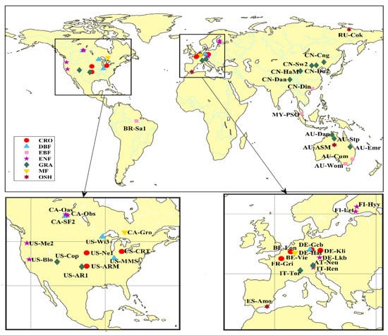
Figure 1.
Location of the 43 FLUXNET sites. The biomes types are identified based on the International Geosphere-Biosphere Programme (IGBP) biome classification.
At the catchment scale, the water balance dataset for 32 major (i.e., >200,000 km2) river catchments developed by Pan et al. [56] was used to evaluate the model performance at regional scale. This data sets merged a number of global datasets including in situ observations (CPC, CPU, GPCC, WM, and CRDC), remote sensing retrievals (GRACE and SEBS), land surface model simulations (VIC), and global reanalyzes (ERA-interim) using data assimilation techniques. This dataset is considered to be the best available water budget dataset [57,58], and includes monthly precipitation, ET, streamflow, and the change in water storage from 1984 to 2006. The main information and statistical parameters of the observed ET data across 32 catchments were given in Supplementary Table S4. The SD values varied from 6.65 mm/month to 36.55 mm/month. The skewness values at most catchments were within the acceptable limit of ± 2, and the kurtosis values of most catchments were lower than 3.
At the global scale, the model tree ensembles (MTE) product [15] spans from 1982 to 2011 at monthly temporal resolution and 0.5° spatial resolution. The MTE model integrates observed ET at the FLUXNET sites with satellite remote sensing and surface meteorological data in a machine-learning algorithm. It is widely used for the comparison and verification of model performances [4,41,59]. The Global Land Evaporation Amsterdam Model (GLEAM) calculates ET from satellite observations based on the P-T equation [17] and performed well in ET estimates [17,27].
2.4. Analysis Method
The statistical measures used to evaluate model performance include the slope of the regression line, the coefficient of determination (R2), root-mean-square error (RMSE), mean absolute error (MAE), and the Nash–Sutcliffe efficiency coefficient (NSE) [60]. The R2 describes the degree of co-linearity between observed and simulated values and ranges between 0 and 1. Generally, an R2 > 0.5 is considered as acceptable performance [61]. The RMSE, MAE, and NSE were computed as:
where O(t) is the observed ET, S(t) is the simulated ET, and Ō is the mean of observed values. The NSE is a normalized statistic that determines the relative magnitude of the residual variance compared to the measured data variance. NSE values range between −∞ to 1. When the NSE values is closer to 1, the simulation is better. The RMSE and MAE show the magnitude and variance in error between observed and simulated values, both ranging from 0 to +∞.
3. Results
3.1. Model Evaluation at Local Scale
The model performances on monthly estimated ET driving by different inputs data were compared with the observations from 43 Fluxnet sites (Figure 2). The SiTH model overestimated ET when using all the forcing datasets. The linear regression slope between observed and simulated ET ranged from 1.18 to 1.25, especially for the MERRA-2 (slope = 1.23~1.25). The R2 between observed and estimated ET for SiTH were highest (R2 > 0.73) among the three models, suggesting that the estimated ET by SiTH had a better consistency with the observed ET. When the same LAI data was used, the estimated ET by SiTH using ERA-5 data was better than that using MERRA-2 data (Figure 2). When the same meteorological data was used, there were little differences in simulated ET between different LAI datasets (Figure 2). Thus, it seemed that the influences of the meteorological data on the performances of SiTH was larger than that of the LAI data (Figure 2). For MOD16 model, the regression slopes between observed and estimated ET were closer to 1 (slope = 0.92~1.0). However, the R2 between observed and simulated ET by MOD16 is generally lower than the other models (R2 = 0.55~0.79), indicating the estimated ET by MOD16 had poor consistencies with observed ET, especially using GLOBMAP LAI data (R2 = 0.55) (Figure 2a,b). Importantly, the uncertainty in LAI had higher influences on the performances of MOD16 model. For PT-JPL model, its performances using MERRA-2 (slope = 0.97~0.99, R2 = 0.70~0.72) were much better than that using ERA-5 (slope = 0.71~0.72, R2 = 0.61~0.66), indicating that meteorological data had greater influences on model performances than LAI data.
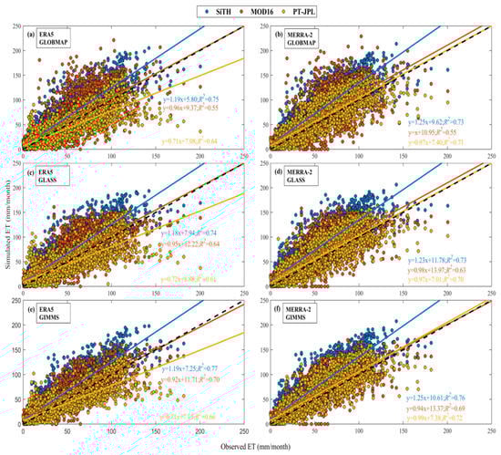
Figure 2.
Scatter plots of the simulated evapotranspiration (ET) of three models using different forcing datasets versus measured ET at 43 flux sites. On the left panels, the same meteorological dataset of ERA5 and leaf area index (LAI) datasets of (a) GLOBMAP, (c) GLASS, and (e) GIMMS was used to simulate ET, respectively. On the right panels, the same meteorological dataset of MERRA-2 and LAI datasets of (b) GLOBMAP, (d) GLASS, and (f) GIMMS was used to estimate ET, respectively. The black dotted line represents the 1:1 line.
Due to the differences in model structure and parameterization, the model performances in ET simulations varied over different land surfaces [22,25,62,63,64,65]. Figure 3 shows the performances of the three models across the different biomes. For the forest biomes, the SiTH model generally overestimated ET, with the mean slope of 1.60, 1.25, 1.28, and 1.67 for ENF, EBF, DBF, and MF, respectively. On the contrary, the MOD16 and PT-JPL models performed relatively well at most forest biomes with the exception of MF, and the mean slope ranged from 0.97 to 1.04 and from 0.81 to 1.05 among these biomes, respectively. However, over the short vegetation types (i.e., GRA, CRO, and OSH), SiTH performed better than MOD16 and PT-JPL, with mean slope of 0.95, 1.01, and 0.95 for GRA, CRO, and OSH, respectively. It was also observed that the MOD16 and PT-JPL significantly underestimated ET in dryland biomes (OSH) (MOD16: slope = 0.25~0.2; PT-JPL: slope = 0.29~0.55) (Figure 3). The values of R2 for the three models were higher than 0.5 over forest biomes, indicating good consistencies between observed and simulated ET. In addition, the SiTH model was satisfactory over short vegetations with R2 ranging from 0.64 to 0.73. However, the MOD16 and PT-JPL models do not capture the ET dynamics in dryland biomes (MOD16: R2 = 0.02~0.12; PT-JPL: R2 = 0.12~0.46). The SiTH model generated negative NSE over most forests, while the PT-JPL model had the NSE values closer to 1. The SiTH model produced high NSE for short vegetations (mean NSE = 0.2~0.47), and the PT-JPL and MOD16 models had the NSE values lower than 0 in OSH. The values of RMSE and MAE for SiTH were significantly higher than that of MOD16 and PT-JPL over forests biomes. Generally, the PT-JPL model had lower values of RMSE and MAE than the other two models for the majority of biomes.
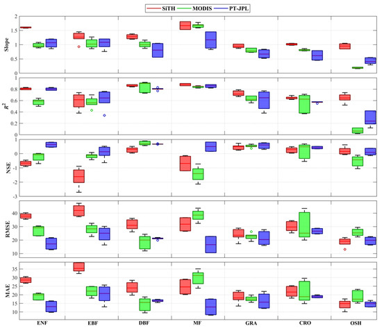
Figure 3.
Comparison of the simulated ET by three models using different forcing datasets versus observed ET at different biomes. Boxplots show the slope, R2 and NSE statistical significance of simulated ET. The central solid line of each box shows the median. The bottom and top of boxes represent the 25th and 75th percentiles, respectively. The lower and upper whiskers indicate the minimum and maximum values, respectively. The circles represent outliers.
3.2. Model Evaluation at Catchment Scale
At regional scale, SiTH tended to overestimate ET driving by different LAI and meteorological data (Figure 4). The regression slope between observed and estimated ET by SiTH ranged from 1.22 to 1.36. The values of R2 for SiTH (0.89~0.90) were generally higher than that for MOD16 and PT-JPL. The MOD16 model also slightly overestimated ET with values of slope being 1.03 to 1.16, and the R2 values were lower than the other two models (R2 = 0.71~0.80). The PT-JPL model performed well with the slope ranging from 0.87 to 1.03 and R2 varying from 0.79 to 0.86. The regression slope between observed and PT-JPL estimated ET ranged from 0.87 to 1.03 with R2 varying from 0.79 to 0.86. For the SiTH and PT-JPL models, the meteorological data has relatively higher influences on simulated ET than LAI data. For the MOD16 model, the estimated ET showed relatively great differences by using different LAI datasets.
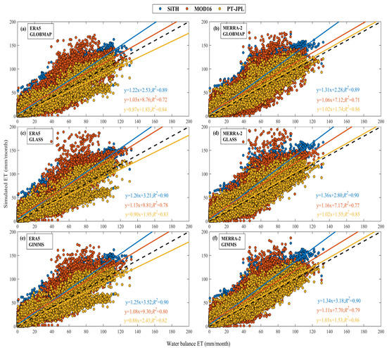
Figure 4.
Scatter plots of the simulated ET by three models using different forcing datasets versus measured ET at 32 catchments. On the left panels, the same meteorological datasets of ERA5 and different LAI datasets of (a) GLOBMAP, (c) GLASS, and (e) GIMMS was used to estimate ET, respectively. On the right panels, the same meteorological datasets of MERRA-2 and different LAI datasets of (b) GLOBMAP, (d) GLASS, and (f) GIMMS was used to estimate ET, respectively. The black dotted line represents the 1:1 line.
The performances of the three models over each basin were compared in Figure 5. Both MOD16 and SiTH models overestimated ET over the majority of the catchments, while PT-JPL performs relatively well in most catchments. The estimated ET by three models (especially SiTH) shows high consistency with water balance ET, with the R2 greater than 0.8 in the majority of catchments. However, the values of R2 in three models are very low in several basins (Amazon, Congo, Mekong, MOD16 in Aral, Indus, Murray and Olenek). The PT-JPL model has a relative good performance in most catchments than the other two models, with greater NSE values (closer to 1), lower RMSE (mean RMSE = 12.44 ± 5.10 month−1), and MAE values (mean MAE = 9.40 ± 4.53 month−1) than SiTH (mean RMSE = 18.95 ± 9.02 month−1, mean MAE = 14.36 ± 8.53 month−1), and MOD16 (mean RMSE = 20.10 ± 10.72 month−1, mean MAE = 16.58 ± 9.33 month−1) in all basins. Generally, the three models performed poorly over catchments in the tropical rainforest areas (Amazon, Congo, and Mekong) and Zhujiang region. In addition, MOD16 also performed poorly in high latitudes regions (Indigirk, Olenek, and Yukon). This may be due to large discrepancies of LAI and meteorological data sets [36,39] or to a lack of a robust description of snow and ice evaporation at high latitudes.
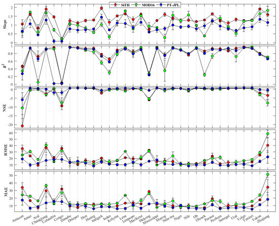
Figure 5.
Comparison of the simulated ET of three models versus water balance ET at 32 catchments. The bottom, middle, and top panels represent the slope, R2, and NSE, respectively. The dots are the median of simulated ET under different forcing datasets. Error bar illustrates the mean ± 1 s.d.
3.3. Evaluation of ET at Global Scales
At global scale, we calculated the average annual ET during 1982–2011 using these models forced by six different combinations of inputs (Figure 6). The spatial pattern of simulated ET by the three models were very similar. The highest annual ET was found over the amazon basin, the Congo rainforest and the southeast Asia near the equator, while the lowest annual ET were in the north Africa, most areas of central Asia, the southwestern United States, central and western Australia, and some parts of high latitude. The average total annual ET from 1982 to 2011 were (76.87 ± 2.98) × 103 km3, (71.68 ± 2.82) × 103 km3, and (61.25 ±1.92) × 103 km3 for SiTH, MOD16, and PT-JPL model, respectively. These values fell in the ranges from 54.9 × 10³ km3 to 85 × 103 km3 reported by previous studies [2,28,66,67]. In addition, the mean annual global land ET calculated from MET and GLEAM during the same period were 63.34 × 10³ km3 and 65.7 × 10³ km3, respectively. These values were slightly lower than that estimated by SiTH and MOD16 model, but very close to that estimated by PT-JPL model. The latitudinal average of ET simulated by the three model during 1982–2011 were also presented Figure 6 and showed similar latitudinal pattern. Relative high ET values were observed near the equator area and near 20°N. However, the estimated ET in tropical regions by SiTH model was higher than that estimated by the other two models. The PT-JPL estimated ET was relatively low for the latitudes 30–60°N, and estimated ET by MOD16 was low for the latitudes between 15°S and 30°S [22].
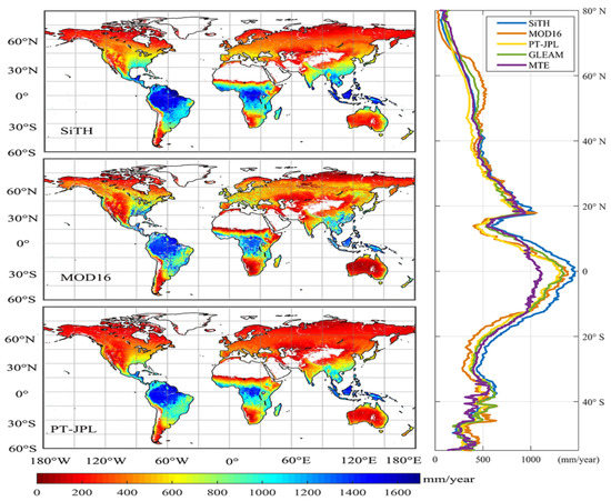
Figure 6.
Spatial patterns of annual mean land evapotranspiration for the SiTH, MOD16, PT-JPL, MTE, and GLEAM from 1982 to 2011. The right panel shows the latitudinal profiles of ET from each model between 55°S and 80°N.
Figure 7 shows the ensembles of multi-decadal ET anomalies (1982–2017) using three process-based ET models forced by the six different combinations of inputs. Generally, the range of the ensembles of global ET anomalies shows large fluctuations, and the median of long-term global ET ensembles agreed better with the global ET trend by MET (Figure 7a). There were two peaks in the median of global ET ensembles in 1998 (median ET anomalies = 17.17 mm/year) and 2010 (median ET anomalies = 14.79 mm/year), respectively. Both 1998 and 2010 were El Niño years. There was an increasing trend from 1982 to 1998, and a decreasing trend from 1998 to 2008. After 2008, the ET reached its second summit in 2010. Since the summit in 2010, the global ET fluctuantly declined but reached high positive anomaly in 2016.
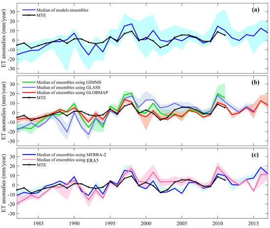
Figure 7.
Global land ET anomalies. (a) Ensembles of global ET anomalies from 1982 to 2017 under all models and the forcing datasets. (b) The estimates of ET anomalies from three LAI datasets with different combinations of models and meteorological datasets. The green line (GIMMS), blue line (GLASS), and red line (GLOBMAP) represent the median of ET ensembles using the GIMMS, GLASS, and GLOBMAP LAI datasets, respectively. (c) The estimates of ET anomalies from two meteorological datasets with different combinations of models and LAI datasets. The blue line (MERRA-2) and pink line (ERA5) is the median of ET ensembles using the MERRA-2 and ERA5, respectively. The shading area indicates the inter-quartile of ET ensembles using different LAI and meteorological datasets.
To evaluate the impact of LAI and meteorological data uncertainties on long-term ET trend, we classified 18 sets of ET products in Supplementary Table S2 into the following two categories: (1) the estimates of ET from three LAI datasets with different combinations of models and meteorological datasets, which were mainly used to investigate the influences of different LAI datasets on the ET estimations (Figure 7b); and (2) the estimates of ET from two meteorological datasets with different combinations of models and LAI datasets, which were mainly used to investigate the influences of different meteorological datasets on ET estimations (Figure 7c). In Figure 7b, the estimates of ET using the GLASS dataset deviated from those using the GLOBMAP and GIMMS datasets. The estimated ET using the GLASS dataset were lower than those by the other two LAI datasets during the 1988–1993 period, while the estimated ET using the GLASS dataset were higher than those by the other two LAI datasets during 1999–2004 period. In Figure 7c, the estimates of ET using the MERRA-2 dataset were very similar to that using the ERA5 data, and their inter-quartile range of ET overlapped greatly and varied synchronously. Also, the median values of ensembles ET using the ERA5 and MERRA-2 datasets were consistent with the ET value estimated by MET.
4. Discussion
4.1. Analyzing the Performance of Models
The three models with different structural complexity and process parameterizations have been developed to predict global ET. Hence, these models are expected to present various performance in estimating ET [21,43]. In this study, we found that the SiTH model overestimated ET over some specific biomes (i.e., forest) and in tropical regions. However, this model exhibited relatively high consistency with the observations (R2 = 0.6~0.88). In this model, the P-T coefficient α is a dimensionless factor associated with the Bowen ratio to limit evaporation, and its value of 1.26 is derived from the data of daily fluxes at saturated land sites and open water [20]. Many studies revealed that the value of α for forests may be below 1.26. For examples, Komatsu et al. [68] reported that the value of α is 0.83 ± 0.15 for deciduous forests and α = 0.63 ± 0.2 for coniferous forests. Cho et al. [69] discovered that the mean value of α for deciduous forests is 1.01 and for the coniferous forests is only 0.75. Luciana et al. [70] found that α values for forests are around 0.65. Therefore, the overestimates of ET by SiTH is due to the high α value used in this model for forest ecosystems. On the contrary, SiTH has a good performance over short vegetation ecosystems (i.e., grassland, cropland and shrubland). For the well-watered short vegetations, the value of α = 1.26 is confirmed in the literature [20]. Pereira et al. [71] reported that the value of α at the irrigated croplands ranged from 1.17 to 1.35. Some researchers found that the value of α close to the 1.26 over shrublands [72,73]. So, the SiTH performed relatively well over short vegetation ecosystems (i.e., grassland, cropland, and shrubland) (Figure 4). Notice that the α value may systematically vary on the daily and seasonal cycles [68,74,75]. So, it should take this variation into account in the future studies and optimize the value of α in SiTH for forests to improve its accuracy in ET simulations.
We also found that both PT-JPL and MOD16 performed poor in dryland biomes (OSH), which is consistent with the previous studies [22,25,27,29,46,59,76,77,78]. In arid areas, soil moisture is the main factor to influences ET processes. However, the PT-JPL and MOD16 models used the atmospheric moisture conditions (i.e., air temperature, RH, and VPD) to reflect soil moisture constraints on ET [10,11,12] rather than directly using the soil moisture to constrain the ET. Novick et al. [79] reported that atmospheric moisture conditions may be significantly correlated with soil moisture at month to year timescales, but they tended to be nearly decoupled at the daily and hourly time scales. Thus, the PT-JPL and MOD16 models using the atmospheric moisture conditions to limit soil moisture may not properly describe the restricts of soil moisture on ET in arid regions. Recently, Purdy et al. [80] proposed to incorporate satellite-observed soil moisture into the PT-JPL model, and great improvements in model performances were obtained especially in water-limited regions. Furthermore, the soil moisture constraint was calculated as RHVPD/β in MOD16 and PT-JPL models. The parameter β is the sensitivity of soil moisture constraint to VPD, and plays an important role in accurate estimation of soil evaporation [12,27,46,59,76]. Zhang et al. [29,46] found that β was the most sensitive parameter, and its values in arid area were lower than that in humid regions, resulting in low soil evaporation due to soil moisture stress. On the contrary, the SiTH model directly uses soil water content to describe soil moisture limitation, and performs relatively well in arid areas [18]. Finally, plants have deep roots in arid regions [81,82] and can utilize deeper soil moisture or even groundwater to maintain growth [83]. However, only SiTH among the three models took the influences of groundwater into account during ET modeling.
4.2. Impact of the Uncertainties of Forcing Data on ET
Models tend to exhibit different behavior when forced with different input data [22,25,30,84]. From the evaluation of monthly estimated ET by the three models using different combinations of forcing datasets at local and regional scales (Figure 2 and Figure 4), the SiTH model overestimated ET with all forcing datasets. Using different meteorological datasets, the differences of simulated ET by SiTH model were relatively larger than using different LAI datasets. A slight improvement in performances were observed by using ERA5 meteorological dataset. Also, it seemed that the estimated ET by MOD16 model was more sensitive to LAI datasets than meteorological datasets. For the PT-JPL model, the uncertainty in meteorological data had large influence on the estimated ET than LAI data, and relatively good performances were found using MERRA-2.
Moreover, the differences were found in estimated global ET anomalies by three models using different combination of forcing datasets, but the ensemble median of global ET anomalies agreed well with the MTE-estimated global land ET anomalies (Figure 7a). It indicates that the ensemble-model method can well capture the uncertainties in ET estimates [22,25,34,43]. Generally, the global ET shows an increasing trend from 1982 to 1998. After the summit in 1998, global ET shows a decreasing trend from 1998 to 2008 (Figure 7a). This agrees well with the results of previous studies [2,40,41,42]. Some authors thought that the decline in global ET from 1998 to 2008 was caused by ENSO-induced anomalous dry conditions and consequent limited moisture supply, especially in the Southern Hemisphere [2,42]. However, the decline of ET was transient, and global land ET reached another summit in 2010 (Figure 7a). It demonstrated a transition from El Niño phase to the La Niña phase in 2010 with high precipitation [85], leading to a high ET [42]. Thus, the decline of ET after 1998 was a transient variation but not a constant decline signal. In the future, more studies are needed to figure out the mechanisms in controlling the long-term variations of global ET.
Comparing the global ET anomalies at annual scale under different forcing datasets, we found that the estimated ET anomalies using the GLASS dataset showed large inconsistency with those using the GIMMS and GLOBMAP LAI datasets. Thus, it seemed that the GLOBMAP and GIMMS datasets were more suitable for long-term ET simulations than the GLASS dataset. This is consistent with previous studies. For example, Jiang et al. [36] found that interannual variabilities of GLASS LAI products show large differences with other LAI products (i.e., GLOBMAP, GIMMS, and TCDR). Furthermore, previous studies found that vegetation greening is main driver to the multi-decadal ET trend since 1980s [40,86,87,88,89]. Therefore, great disagreements among global long-term satellite LAI products can cause the large differences of estimated long-term ET trend. The differences of estimated ET anomalies using the different meteorological datasets was relatively small (Figure 7c). The ensemble median values of global ET using ERA5 and MERRA-2 datasets are in agreement with the MTE-estimated global land ET anomalies. Thus, it seemed that the influences of meteorological datasets on global ET estimates can be ignored partially due to their relatively good qualities.
5. Conclusions
In this study, we evaluated the performances of three process-based ET models in ET simulations at multiple scales by using various LAI and meteorological forcing datasets. The results showed that SiTH simulated well in dryland short vegetation ecosystems but overestimated ET in forest ecosystems because the P-T coefficient (α) may be set too high in this model. The PT-JPL and MOD16 models performed well in forests, but poorly in dryland biomes due to their improper description of soil moisture stress based on atmospheric moisture conditions. Similar model performances were observed at both catchment and global scales. To obtain proper long-term global ET estimates, the multi-model ensemble approach is a proper choice. We found that the ensembles median of global ET anomalies from different models and forcing datasets showed good consistency with that obtained by the MTE method. Generally, the uncertainty of LAI datasets has larger influences on the global ET estimates than the meteorological datasets. Thus, we should pay more attention to research global changes derived from the global LAI products. In further studies, we should optimize the P-T coefficient (α) over different vegetation types for SiTH to improve its accuracy in ET simulations over forest ecosystems. Finally, more studies are need to quantify the contributions of different driving factors to the variations in global ET and to figure out the mechanisms in controlling global ET changes.
Supplementary Materials
The following are available online at https://www.mdpi.com/2072-4292/12/15/2473/s1, Table S1: Variables used as input to derive evapotranspiration (ET) in three models, Table S2: Details of the input datasets combinations for each ensemble members, Table S3: The monthly statistical parameters of the measured ET data at flux sites, and Table S4: The main characteristics and monthly statistical parameters at the 32 catchments.
Author Contributions
Conceptualization, G.Z. and X.J.; methodology, S.S.; validation, Y.Z. and W.Q.; investigation, B.D.; data curation, N.Z.; writing—original draft preparation, H.C.; writing—review and editing, H.C., G.Z., K.Z. and J.B. All authors have read and agreed to the published version of the manuscript.
Funding
This research was funded by the National Key Research and Development Program of China (2018YFC0406602) and the National Natural Science Foundation of China (41871078).
Acknowledgments
We thank all the principal investigators and their teams of all the dataset used in this study. This work used eddy covariance data acquired and shared by the FLUXNET community, including these networks: AmeriFlux, AfriFlux, AsiaFlux, CarboAfrica, CarboEuropeIP, CarboItaly, CarboMont, ChinaFlux, Fluxnet-Canada, GreenGrass, ICOS, KoFlux, LBA, NECC, OzFlux-TERN, TCOS-Siberia, and USCCC, available at https://fluxnet.fluxdata.org. The water balance datasets are provided by Pan Ming et al. The GLOBMAP datasets are available at http://www.globalmapping.org/. The GLASS datasets are acquired from http://www.glcf.umd.edu/. The MERRA-2 reanalysis datasets are available at https://disc.sci.gsfc.nasa.gov. The ERA5 reanalysis datasets are acquired from https://cds.climate.copernicus.eu/. The MCD12C1 products used in this study are available at https://lpdaac.usgs.gov/. The GLEAM datasets are available at https://www.gleam.eu/. The MTE datasets are acquired from http://www.bgc-jena.mpg.de/geodb/.
Conflicts of Interest
The authors declare no conflict of interest.
References
- Trenberth, K.E.; Fasullo, J.T.; Kiehl, J. Earth’s global energy budget. Bull. Am. Meteorol. Soc. 2009, 90, 311–323. [Google Scholar] [CrossRef]
- Jung, M.; Reichstein, M.; Ciais, P.; Seneviratne, S.I.; Sheffield, J.; Goulden, M.L.; Bonan, G.; Cescatti, A.; Chen, J.Q.; de Jeu, R.; et al. Recent decline in the global land evapotranspiration trend due to limited moisture supply. Nature 2010, 467, 951–954. [Google Scholar] [CrossRef]
- Wang, K.C.; Dickinson, R.E. A review of global terrestrial evapotranspiration:observation, modeling, climatology, and climatic variability. Rev. Geophys. 2012, 50. [Google Scholar] [CrossRef]
- Miralles, D.G.; Van Den Berg, M.J.; Gash, J.H.; Parinussa, R.M.; De Jeu, R.A.; Beck, H.E.; Holmes, T.R.; Jiménez, C.; Verhoest, N.E.; Dorigo, W.A. El Niño–La Niña cycle and recent trends in continental evaporation. Nat. Clim. Chang. 2014, 4, 122–126. [Google Scholar] [CrossRef]
- Fisher, J.B.; Melton, F.; Middleton, E.; Hain, C.; Anderson, M.; Allen, R.; McCabe, M.F.; Hook, S.; Baldocchi, D.; Townsend, P.A.; et al. The future of evapotranspiration: Global requirements for ecosystem functioning, carbon and climate feedbacks, agricultural management, and water resources. Water Resour. Res. 2017, 53, 2618–2626. [Google Scholar] [CrossRef]
- Norman, J.M.; Kustas, W.P.; Humes, K.S. Source approach for estimating soil and vegetation energy fluxes in observations of directional radiometric surface-temperature. Agric. For. Meteorol. 1995, 77, 263–293. [Google Scholar] [CrossRef]
- Bastiaanssen, W.G.M.; Menenti, M.; Feddes, R.A.; Holtslag, A.A.M. A remote sensing surface energy balance algorithm for land (SEBAL). 1. Formulation. J. Hydrol. 1998, 212, 198–212. [Google Scholar] [CrossRef]
- Su, Z. The Surface Energy Balance System (SEBS) for estimation of turbulent heat fluxes. Hydrol. Earth Syst. Sci. 2002, 6, 85–99. [Google Scholar] [CrossRef]
- Cleugh, H.A.; Leuning, R.; Mu, Q.; Running, S.W. Regional evaporation estimates from flux tower and MODIS satellite data. Remote Sens. Environ. 2007, 106, 285–304. [Google Scholar] [CrossRef]
- Mu, Q.Z.; Heinsch, F.A.; Zhao, M.; Running, S.W. Development of a global evapotranspiration algorithm based on MODIS and global meteorology data. Remote Sens. Environ. 2007, 111, 519–536. [Google Scholar] [CrossRef]
- Mu, Q.Z.; Zhao, M.; Running, S.W. Improvements to a MODIS global terrestrial evapotranspiration algorithm. Remote Sens. Environ. 2011, 115, 1781–1800. [Google Scholar] [CrossRef]
- Fisher, J.B.; Tu, K.P.; Baldocchi, D.D. Global estimates of the land–atmosphere water flux based on monthly AVHRR and ISLSCP-II data, validated at 16 FLUXNET sites. Remote Sens. Environ. 2008, 112, 901–919. [Google Scholar] [CrossRef]
- Fisher, J.B.; Lee, B.; Purdy, A.J.; Halverson, G.H.; Dohlen, M.B.; Cawse-Nicholson, K.; Wang, A.; Anderson, R.G.; Aragon, B.; Arain, M.A.; et al. ECOSTRESS: NASA’s Next Generation Mission to Measure Evapotranspiration from the International Space Station. Water Resour. Res. 2020, 56, e2019WR026058. [Google Scholar] [CrossRef]
- Leuning, R.; Zhang, Y.Q.; Rajaud, A.; Cleugh, H.; Tu, K. A simple surface conductance model to estimate regional evaporation using MODIS leaf area index and the Penman-Monteith equation. Water Resour. Res. 2008, 44, 652–655. [Google Scholar] [CrossRef]
- Jung, M.; Reichstein, M.; Bondeau, A. Towards global empirical upscaling of FLUXNET eddy covariance observations: Validation of a model tree ensemble approach using a biosphere model. Biogeosciences 2009, 6, 2001–2013. [Google Scholar] [CrossRef]
- Zhang, K.; Kimball, J.S.; Nemani, R.R.; Running, S.W. A continuous satellite-derived global record of land surface evapotranspiration from 1983 to 2006. Water Resourc Res. 2010, 46, W09522. [Google Scholar] [CrossRef]
- Miralles, D.G.; De Jeu, R.A.M.; Gash, J.H.; Holmes, T.R.H.; Dolman, A.J. Magnitude and variability of land evaporation and its components at the global scale. Hydrol. Earth Syst. Sci. 2011, 15, 967–981. [Google Scholar] [CrossRef]
- Zhu, G.F.; Zhang, K.; Chen, H.L.; Wang, Y.Q.; Sun, Y.H.; Zhang, Y.; Ma, J.Z. Development and evaluation of a simple hydrologically based model for terrestrial evapotranspiration simulations. J. Hydrol. 2019, 577. [Google Scholar] [CrossRef]
- Monteith, J.L. Evaporation and Environment, in The State and Movement of Water in Living Organisms; Symposium of the Society of Experimental Biology; Cambridge University Press: Cambridge, UK, 1965; pp. 205–234. [Google Scholar]
- Priestley, C.H.B.; Taylor, R.J. On the assessment of surface heat flux and evaporation using large-scale parameters. Mon. Weather Rev. 1972, 100, 81–92. [Google Scholar] [CrossRef]
- Vinukollu, R.K.; Meynadier, R.; Sheffield, J.; Wood, E.F. Multi-model, multi-sensor estimates of global evapotranspiration: Climatology, uncertainties and trends. Hydrol. Process. 2011, 25, 3993–4010. [Google Scholar] [CrossRef]
- Vinukollu, R.K.; Wood, E.F.; Ferguson, C.R.; Fisher, B. Global Estimates of Evapotranspiration for Climate Studies using Multi-Sensor Remote Sensing Data: Evaluation of Three Process-Based Approaches. Remote Sens. Environ. 2011, 115. [Google Scholar] [CrossRef]
- Long, D.; Longuevergne, L.; Scanlon, B.R. Uncertainty in evapotranspiration from land surface modeling, remote sensing, and GRACE satellites. Water Resour. Res. 2014, 50, 1131–1151. [Google Scholar] [CrossRef]
- Ramoelo, A.; Majozi, N.; Mathieu, R.; Jovanovic, N.; Nickless, A.; Dzikiti, S. Validation of Global Evapotranspiration Product (MOD16) using Flux Tower Data in the African Savanna, South Africa. Remote Sens. 2014, 6, 7406–7423. [Google Scholar] [CrossRef]
- Ershadi, A.; McCabe, M.F.; Evans, J.P.; Chaney, N.W.; Wood, E.F. Multi-site evaluation of terrestrial evaporation models using FLUXNET data. Agr. For. Meteorol. 2014, 187, 46–61. [Google Scholar] [CrossRef]
- Ershadi, A.; McCabe, M.F.; Evans, J.P.; Wood, E.F. Impact of model structure and parameterization on Penman–Monteith type evaporation models. J. Hydrol. 2015, 525, 521–535. [Google Scholar] [CrossRef]
- Michel, D.; Jiménez, C.; Miralles, D.G.; Jung, M.; Hirschi, M.; Ershadi, A.; Martens, B.; McCabe, M.F.; Fisher, J.B.; Mu, Q.Z.; et al. The WACMOS-ET project & ndash; Part 1: Towerscale evaluation of four remote-sensing-based evapotranspiration algorithms. Hydrol. Earth Syst. Sci. 2016, 20, 803–822. [Google Scholar] [CrossRef]
- Miralles, D.G.; Jiménez, C.; Jung, M.; Michel, D.; Ershadi, A.; McCabe, M.F.; Hirschi, M.; Martens, B.; Dolman, A.J.; Fisher, J.B.; et al. The WACMOS-ET project & ndash; Part 2: Evaluation of global terrestrial evaporation data sets. Hydrol. Earth Syst. Sci. 2016, 20, 823–842. [Google Scholar] [CrossRef]
- Zhang, K.; Zhu, G.F.; Ma, J.Z.; Yang, Y.Q.; Shang, S.S.; Gu, C.J. Parameter analysis and estimates for the MODIS evapotranspiration algorithm andmultiscale verification. Water Resour. Res. 2019, 55, 2211–2231. [Google Scholar] [CrossRef]
- Badgley, G.; Fisher, J.B.; Jiménez, C.; Tu, K.P.; Vinukollu, R.K. On uncertainty in global evapotranspiration estimates from choice of input forcing datasets. J. Hydrometeorol. 2015, 16, 1449–1455. [Google Scholar] [CrossRef]
- Good, S.P.; Noone, D.; Bowen, G. Hydrologic connectivity constrains partitioning of global terrestrial water fluxes. Science 2015, 349, 175–177. [Google Scholar] [CrossRef]
- Wang, L.; Good, S.P.; Caylor, K.K. Global synthesis of vegetation control on evapotranspiration partitioning. Geophys. Res. Lett. 2014, 41, 6753–6757. [Google Scholar] [CrossRef]
- Kala, J.; Decker, M.; Exbrayat, J.; Pitman, A.J.; Carouge, C.; Evans, J.P.; Abramowitz, G.; Mocko, D. Influence of Leaf Area Index Prescriptions on Simulations of Heat, Moisture, and Carbon Fluxes. J. Hydrometeor. 2014, 15, 489–503. [Google Scholar] [CrossRef]
- Zhang, K.; Kimball, J.S.; Running, S.W. A review of remote sensing based actual evapotranspiration estimation. Wiley Interdiscip. Rev. Water 2016, 3, 834–853. [Google Scholar] [CrossRef]
- Chen, J.M.; Ju, W.; Ciais, P.; Viovy, N.; Liu, R.; Liu, Y.; Lu, X. Vegetation structural change since 1981 significantly enhanced the terrestrial carbon sink. Nat Commun. 2019, 10, 4259. [Google Scholar] [CrossRef] [PubMed]
- Jiang, C.; Ryu, Y.; Fang, H.; Myneni, R.; Claverie, M.; Zhu, Z. Inconsistencies of interannual variability and trends in long-term satellite leaf area index products. Glob. Chang. Biol. 2017, 23, 4133–4146. [Google Scholar] [CrossRef]
- Zhu, Z.; Piao, S.; Myneni, R.B.; Huang, M.; Zeng, Z.; Canadell, J.G.; Ciais, P.; Sitch, S.; Friedlingstein, P.; Arneth, A.; et al. Greening of the Earth and its drivers. Nat. Clim. Chang. 2016, 6, 791–795. [Google Scholar] [CrossRef]
- IPCC. Summary for Policymakers. In Global Warming of 1.5 °C; An IPCC Special Report on the impacts of global warming of 1.5 °C above pre-industrial levels and related global greenhouse gas emission pathways, in the context of strengthening the global response to the threat of climate change, sustainable development, and efforts to eradicate poverty; World Meteorological Organization: Geneva, Switzerland, 2018; p. 32. [Google Scholar]
- Jia, A.; Liang, S.; Jiang, B.; Zhang, X.; Wang, G. Comprehensive assessment of global surface net radiation products and uncertainty analysis. J. Geophys. Res. Atmos. 2018, 123, 1970–1989. [Google Scholar] [CrossRef]
- Zhang, K.; Kimball, J.; Nemani, R.; Running, S.W.; Hong, Y.; Gourley, J.J.; Yu, Z. Vegetation Greening and Climate Change Promote Multidecadal Rises of Global Land Evapotranspiration. Sci. Rep. 2015, 5, 15956. [Google Scholar] [CrossRef]
- Zhang, Y.Q.; Peña-Arancibia, J.L.; McVicar, T.R.; Chiew, F.H.; Vaze, J.; Liu, C.; Lu, X.; Zheng, H.; Wang, Y.; Liu, Y.Y.; et al. Multi-decadal trends in global terrestrial evapotranspiration and its components. Sci. Rep. 2016, 6, 19124. [Google Scholar] [CrossRef]
- Yan, H.; Yu, Q.; Zhu, Z.C.; Myneni, R.B.; Yan, H.M.; Wang, S.Q.; Shugart, H.H. Diagnostic analysis of interannual variation of global land evapotranspiration over 1982–2011: Assessing the impact of ENSO. J. Geophys. Res. Atmos. 2013, 118, 8969–8983. [Google Scholar] [CrossRef]
- Mueller, B.; Hirschi, M.; Jimenez, C.; Ciais, P.; Dirmeyer, P.A.; Dolman, A.J.; Fisher, J.B.; Jung, M.; Ludwig, F.; Maignan, F.; et al. Benchmark products for land evapotranspiration: LandFlux-EVAL multi-data set synthesis. Hydrol. Earth Syst. Sci. 2013, 17, 3707–3720. [Google Scholar] [CrossRef]
- Javadian, M.; Behrangi, A.; Smith, W.K.; Fisher, J.B. Global Trends in Evapotranspiration Dominated by Increases Across Large Cropland Regions. Remote Sens. 2020, 12, 1221. [Google Scholar] [CrossRef]
- Penman, H.L. Natural evaporation from open water, bare soil and grass. Proc. R. Soc. Lond. A 1948, 193, 120–145. [Google Scholar] [CrossRef]
- Zhang, K.; Ma, J.Z.; Zhu, G.F.; Ma, T.; Han, T.; Feng, L.L. Parameter sensitivity analysis and optimization for a satellite-based evapotranspiration model across multiple sites using Moderate Resolution Imaging Spectroradiometer and flux data. J. Geophys. Res. Atmos. 2017, 122, 230–245. [Google Scholar] [CrossRef]
- Liu, Y.; Liu, R.; Chen, J.M. Retrospective retrieval of long-term consistent global leaf area index (1981–2011) from combined AVHRR and MODIS data. J. Geophys. Res. Biogeosci. 2012, 117, G04003. [Google Scholar] [CrossRef]
- Xiao, Z.; Liang, S.; Wang, J.; Xiang, Y.; Zhao, X.; Song, J. Long-time-series global land surface satellite leaf area index product derived from MODIS and AVHRR surface reflectance. IEEE Trans. Geosci. Remote Sens. 2016, 54, 5301–5318. [Google Scholar] [CrossRef]
- Zhu, Z.; Bi, J.; Pan, Y.; Ganguly, S.; Anav, A.; Xu, L.; Myneni, R.B. Global data sets of vegetation leaf area index (LAI)3g and fraction of photosynthetically active radiation (FPAR)3g derived from global inventory modeling and mapping studies (GIMMS) normalized difference vegetation index (NDVI3G) for the period 1981 to 2011. Remote Sens. 2013, 5, 927–948. [Google Scholar] [CrossRef]
- Gelaro, R.; Mccarty, W.; Suárez, M.J.; Todling, R.; Molod, A.; Takacs, L.; Randles, C.A.; Darmenov, A.; Bosilovich, M.G.; Reichle, R.; et al. The Modern-Era Retrospective Analysis for Research and Applications, Version 2 (MERRA-2). J. Clim. 2017, 30, 5419–5454. [Google Scholar] [CrossRef]
- Hersbach, H.; Dee, D. ERA5 reanalysis is in production. ECMWF Newsl. 2016, 147, 5–6. [Google Scholar]
- Friedl, M.A.; Sulla-Menashe, D.; Tan, B.; Schneider, A.; Ramankutty, N.; Sibley, A.; Huang, X. MODIS Collection 5 global land cover: Algorithm refinements and characterization of new datasets. Remote Sens. Environ. 2010, 114, 168–182. [Google Scholar] [CrossRef]
- Zhao, M.; Heinsch, F.A.; Nemani, R.R.; Running, S.W. Improvements of the MODIS terrestrial gross and net primary production global data set. Remote Sens. Environ. 2005, 95, 164–176. [Google Scholar] [CrossRef]
- Twine, T.E.; Kustas, W.P.; Norman, J.M.; Cook, D.R.; Houser, P.R.; Meyers, T.P.; Prueger, J.H.; Starks, P.J.; Wesely, M.L. Correcting eddy-covariance flux underestimates over a grassland. Agric. For. Meteorol. 2000, 103, 279–300. [Google Scholar] [CrossRef]
- Foken, T.; Wimmer, F.; Mauder, M.; Thomas, C.; Liebethal, C. Some aspects of the energy balance closure problem. Atmos. Chem. Phys. 2006, 6, 4395–4402. [Google Scholar] [CrossRef]
- Pan, M.; Sahoo, A.K.; Troy, T.J.; Vinukollu, R.K.; Sheffield, J.; Wood, E.F. Multisource estimation of long-term terrestrial water budget for major global river basins. J. Clim. 2012, 25, 3191–3206. [Google Scholar] [CrossRef]
- Li, D.; Pan, M.; Cong, Z.; Zhang, L.; Wood, E. Vegetation control on water and energy balance within the Budyko framework. Water Resour. Rese. 2013, 49, 969–976. [Google Scholar] [CrossRef]
- Wang, S.; Pan, M.; Mu, Q.; Shi, X.; Mao, J.; Brümmer, C.; Jassal, R.S.; Krishnan, P.; Li, J.; Black, T.A. Comparing Evapotranspiration from Eddy Covariance Measurements, Water Budgets, Remote Sensing, and Land Surface Models over Canadaa,b. J. Hydrometeorol. 2015, 16, 1038–1041. [Google Scholar] [CrossRef]
- Zhu, G.F.; Zhang, K.; Li, X.; Liu, S.M.; Ding, Z.Y.; Ma, J.Z.; Huang, C.L.; Han, T.; He, J.H. Evaluating the complementary relationship for estimating evapotranspiration using the multi-site data across north China. Agric. For. Meteorol. 2016, 230, 33–44. [Google Scholar] [CrossRef]
- Nash, J.E.; Sutcliffe, J.V. River flow forecasting through conceptual models part I-a discussion of principles. J. Hydrol. 1970, 10, 282–290. [Google Scholar] [CrossRef]
- Moriasi, D.N.; Arnold, J.G.; Van Liew, M.W.; Bingner, R.L.; Harmel, R.D.; Veith, T.L. Model Evaluation Guidelines for Systematic Quantification of Accuracy in Watershed Simulations; American Society of Agricultural Engineers: St. Joseph, MI, USA, 2007; Volume 50, p. 16. [Google Scholar]
- Massman, W.J.; Lee, X. Eddy covariance flux corrections and uncertainties in long-term studies of carbon and energy exchanges. Agric. For. Meteorol. 2002, 113, 121–144. [Google Scholar] [CrossRef]
- Richardson, A.D.; Hollinger, D.Y.; Burba, G.G.; Davis, K.J.; Flanagan, L.B.; Katul, G.G.; William, M.J.; Ricciuto, D.M.; Stoy, P.C.; Suyker, A.E.; et al. A multi-site analysis of random error in tower-based measurements of carbon and energy fluxes. Agric. For. Meteorol. 2006, 136, 1–18. [Google Scholar] [CrossRef]
- Williams, M.; Richardson, A.D.; Reichstein, M.; Stoy, P.C.; Peylin, P.; Verbeeck, H.; Carvalhais, N.; Jung, M.; Hollinger, D.Y.; Kattge, J.; et al. Improving land surface models with FLUXNET data. Biogeosciences 2009, 6, 1341–1359. [Google Scholar] [CrossRef]
- McCabe, M.F.; Ershadi, A.; Jimenez, C.; Miralles, D.G.; Michel, D.; Wood, E.F. The GEWEX LandFlux project: Evaluation of model evaporation using tower-based and globally gridded forcing data. Geosci. Model Dev. 2016, 9, 283–305. [Google Scholar] [CrossRef]
- Oki, T.; Kanae, S. Global hydrological cycles and world water resources. Science 2006, 313, 1068–1072. [Google Scholar] [CrossRef] [PubMed]
- Wang-Erlandsson, L.; van der Ent, R.J.; Gordon, L.J.; Savenije, H.H.G. Contrasting roles of interception and transpiration in the hydrological cycle—Part 1: Temporal characteristics over land. Earth Syst. Dynam. 2014, 5, 441–469. [Google Scholar] [CrossRef]
- Komatsu, H. Forest categorization according to dry-canopy evaporation rates in the growing season: Comparison of the Priestley–Taylor coefficient values from various observation sites. Hydrol. Process. 2005, 19, 3873–3896. [Google Scholar] [CrossRef]
- Cho, J.; Oki, T.; Yeh, P.-F.; Kim, W.; Kanae, S.; Otsuki, K. On the relationship between the Bowen ratio and the near-surface air temperature. Theor. Appl. Climatol. 2012, 108, 135–145. [Google Scholar] [CrossRef]
- Luciana, S.; Carvalho, A.M.D.; Campelo, J.J.H.; Nogueira, J.D.S.; Dalmagro, J.H. Estimativa do coeficiente Priestley-Taylor em floresta monodominante Cambarazal no Pantanal. Rev. Bras. Meteorol. 2010, 25, 448–454. [Google Scholar] [CrossRef][Green Version]
- Pereira, A.R.; Green, S.R.; Villa Nova, N.A. Sap flow, leaf area, net radiation and the Priestley-Taylor formula for irrigated orchards and isolated trees. Agric. Water Manag. 2007, 92, 48–52. [Google Scholar] [CrossRef]
- Owe, M.; Van de Griend, A.A. Daily surface moisture model for large area semi-arid land application with limited climate data. J. Hydrol. 1990, 121, 119–132. [Google Scholar] [CrossRef]
- Caylor, K.K.; Shugart, H.H.; Rodriguez-Iturbe, I. Tree canopy effects on simulated water stress in southern African savannas. Ecosystems 2005, 8, 17–32. [Google Scholar] [CrossRef]
- Assouline, S.; Li, D.; Tyler, S.; Tanny, J.; Cohen, S.; Bou-Zeid, E.; Parlange, M.; Katul, G.G. On the variability of the Priestley-Taylor coefficient over water bodies. Water Resour. Res. 2016, 52, 150–163. [Google Scholar] [CrossRef]
- Tongwane, M.I.; Savage, M.J.; Tsubo, M.; Moeletsi, M.E. Seasonal variation of reference evapotranspiration and Priestley-Taylor coefficient in the eastern Free State, South Africa. Agric. Water Manag. 2017, 187, 122–130. [Google Scholar] [CrossRef]
- García, M.; Sandholt, I.; Ceccato, P.; Ridler, M.; Mougin, E.; Kergoat, L.; Morillas, L.; Timouk, F.; Fensholt, R.; Domingo, F. Actual evapotranspiration in drylands derived from in situ and satellite data: Assessing biophysical constraints. Remote Sens. Environ. 2013, 131, 103–118. [Google Scholar] [CrossRef]
- Sun, J.; Salvucci, G.D.; Entekhabi, D. Estimates of evapotranspiration from MODIS and AMSR-E land surface temperature and moisture over the Southern Great Plains. Remote Sens. Environ. 2012, 127, 44–59. [Google Scholar] [CrossRef]
- Velpuri, N.M.; Senay, G.B.; Singh, R.K.; Bohms, S.; Verdin, J.P. A comprehensive evaluation of two MODIS evapotranspiration products over the conterminous United States: Using point and gridded FLUXNET and water balance ET. Remote Sens. Environ. 2013, 139, 35–49. [Google Scholar] [CrossRef]
- Novick, K.; Ficklin, D.; Stoy, P.; Williams, C.A.; Bohrer, G.; Oishi, A.C.; Papuga, S.A.; Blanken, P.D.; Noormets, A.; Sulman, B.N.; et al. The increasing importance of atmospheric demand for ecosystem water and carbon fluxes. Nat. Clim. Chang. 2016, 6, 1023–1027. [Google Scholar] [CrossRef]
- Purdy, A.J.; Fisher, J.B.; Goulden, M.L.; Colliander, A.; Halverson, G.; Tu, K.; Famiglietti, J.S. SMAP soil moisture improves global evapotranspiration. Remote Sens. Environ. 2018, 219, 1–14. [Google Scholar] [CrossRef]
- Fan, Y.; Li, H.; Miguez-Macho, G. Global patterns of groundwater table depth. Science 2013, 339, 940–943. [Google Scholar] [CrossRef]
- Fan, Y.; Miguez-Macho, G.; Jobbágy, E.G.; Jackson, R.B.; Otero-Casal, C. Hydrologic regulation of plant rooting depth. Proc. Natl. Acad. Sci. USA 2017, 114, 10572–10577. [Google Scholar] [CrossRef]
- Thompson, S.E.; Harman, C.J.; Konings, A.G.; Sivapalan, M.; Neal, A.; Troch, P.A. Comparative hydrology across AmeriFlux sites: The variable roles of climate, vegetation, and groundwater. Water Resour. Res. 2011, 47, W00J07. [Google Scholar] [CrossRef]
- Ferguson, C.R.; Sheffield, J.; Wood, E.F.; Gao, H. Quantifying uncertainty in a remote sensing-based estimate of evapotranspiration over continental USA. Int. J. Remote Sens. 2010, 31, 3821–3865. [Google Scholar] [CrossRef]
- Poulter, B.; Frank, D.; Ciais, P.; Myneni, R.B.; Andela, N.; Bi, J.; Broquet, G.; Canadell, J.G.; Chevallier, F.; Liu, Y.Y.; et al. Contribution of semi-arid ecosystems to interannual variability of the global carbon cycle. Nature 2014, 509, 600–603. [Google Scholar] [CrossRef] [PubMed]
- Polhamus, A.; Fisher, J.B.; Tu, K.P. What controls the error structure in evapotranspiration models? Agric. For. Meteorol. 2013, 169, 12–24. [Google Scholar] [CrossRef]
- Zeng, Z.; Peng, L.; Piao, S. Response of terrestrial evapotranspiration to Earth’s greening. Curr. Opin. Environ. Sustain. 2018, 33, 9–25. [Google Scholar] [CrossRef]
- Forzieri, G.; Miralles, D.G.; Ciais, P.; Alkama, R.; Ryu, Y.; Duveiller, G.; Zhang, K.; Robertson, E.; Kautz, M.; Martens, B.; et al. Increased control of vegetation on global terrestrial energy fluxes. Nat. Clim. Chang. 2020, 10, 356–362. [Google Scholar] [CrossRef]
- Piao, S.; Wang, X.; Park, T.; Chen, C.; Lian, X.; He, Y.; Bjerke, J.W.; Chen, A.; Ciais, P.; Tømmervik, H.; et al. Characteristics, drivers and feedbacks of global greening. Nat. Rev. Earth Environ. 2020, 1, 14–27. [Google Scholar] [CrossRef]


© 2020 by the authors. Licensee MDPI, Basel, Switzerland. This article is an open access article distributed under the terms and conditions of the Creative Commons Attribution (CC BY) license (http://creativecommons.org/licenses/by/4.0/).