A Comparison of SSEBop-Model-Based Evapotranspiration with Eight Evapotranspiration Products in the Yellow River Basin, China

Abstract

Accurate evapotranspiration (ET) estimation is important in understanding the hydrological cycle and improving water resource management. The operational simplified surface energy balance (SSEBop) model can be set up quickly for the routine monitoring of ET. Several studies have suggested that the SSEBop model, which can simulate ET, has performed inconsistently across the United States. There are few detailed studies on the evaluation of ET simulated by SSEBop in other regions. To explore the potential and application scope of the SSEBop model, more evaluation of the ET simulated by SSEBop is clearly needed. We calculated the SSEBop-model-based ET (ET_SSEBopYRB) with land surface temperature product of MOD11A2 and climate variables as inputs for the Yellow River Basin (YRB), China. We also compared the ET_SSEBopYRB with eight coarse resolution ET products, including China ET_MTE, produced using the upscaling energy flux method; China ET_CR, which is generated using the non-linear complementary relationship model; three global products based on the Penman–Monteith logic (ET_PMLv2, ET_MODIS, and ET_BESS), two global ET products based on the surface energy balance (ET_SEBS, ET_SSEBopGlo), and integrated ET products based on the Bayesian model averaging method (ET_GLASS), using the annual ET data derived from the water balance method (WB-ET) for fourteen catchments. We found that ET_SSEBopYRB and the other eight ET products were able to explain 23 to 52% of the variability in the water balance ET for fourteen small catchments in the YRB. ET_SSEBopYRB had a better agreement with WB-ET than ET_SEBS, ET_MODIS, ET_CR, and ET_GLASS, with lower RMSE (88.3 mm yr⁻¹ vs. 121.7 mm yr⁻¹), higher R² (0.49 vs. 0.43), and lower absolute RPE (−3.3% vs. –19.9%) values for the years 2003–2015. We also found that the uncertainties of the spatial patterns of the average annual ET values and the ET trends were still large for different ET products. Third, we found that the free global ET product derived from the SSEBop model (ET_SSEBopGlo) highly underestimated the annual total ET trend for the YRB. The poor performance of the land surface temperature product of MOD11A2 in 2015 caused the large ET_SSEBopYRB uncertainty at eight-day and monthly scales. Further evaluation of ET based on the SSEBop model for site measurements is needed.

1. Introduction

Evapotranspiration (ET) is an essential water flux that connects the soil, vegetation, and atmosphere. The estimation of ET helps us understand the hydrological cycle, improve water resource management [1], and enhance decision support [2], especially in water-limited areas, where water resource competition among agriculture, the social economy, and the environment is more intense [3,4].

Although it is difficult to accurately calculate ET due to the spatial heterogeneity and complex processes involved at regional and global scales [5], there are many methods for estimating ET, which can be categorized into seven main groups: (1) field observations; (2) coupled-process models [6]; (3) remote sensing [7,8]; (4) the meteorologically-based complementary relationship methods [9]; (5) water-balance-based methods [10]; (6) empirical formulae [11]; and (7) machine learning [12]. Surface energy balance algorithms based on remote sensing images are widely used to estimate ET [13,14,15,16]. The operational simplified surface energy balance (SSEBop) model was specifically designed to monitor long-term ET using minimum remote sensing and weather inputs, and has clear advantages over other thermal ET models in terms of operational uses [17]. Although the designation of SSEBop as a surface energy balance model has been criticized due to not resolving the full surface energy balance components [17], it has been successfully used to estimate wheat ET [18], soybean ET [19], and sorghum ET [20], separating blue and green water resources of the coterminous United States (CONUS) [21]; water stress [22]; and long-term regional ET estimates in the whole CONUS [8], the southwestern United States [23], the Midwestern United States [24], the Colorado River Basin of the United States [25], the Nile Basin of Africa [26,27], the Mara Basin of East Africa [28], the arid region of Chile [29], and Ethiopia [30], Landsat images and moderate-resolution imaging spectroradiometer(MODIS) datasets as inputs.

Extensive evaluation of ET estimates is necessary before they are used in various applications [31]. A comprehensive evaluation of SSEBop and MODIS ET over the CONUS indicated that SSEBop showed better performance for grassland and forest classes and effectively reproduced the basin-scale ET response [31]. Singh et al. (2013) estimated the Colorado River Basin ET by applying Landsat images and SSEBop, finding that the SSEBop model captured the annual ET variability well at the site level and sub-basin level [25]. Other research has also reported that the SSEBop model performed well over the CONUS, with an R² of 0.86 between the estimated ET and the ET of 42 flux tower sites from 2001 to 2007 [32]. In the Midwestern United States, the validation of estimated ET by SSEBop using Landsat images captured the spatial and temporal variations in ET, with a low root mean square error and high R². However, SSEBop was consistently the worst-performing model among SEBAL, METRIC, S-SEBI, SEBS, and SSEBop, and it overestimated ET at all sites when estimating humid southeastern United States ET by Landsat imaging from 2000 to 2010 [33], indicating its limited applicability in the southeastern US. A sensitivity research of SSEBop ET in the CONUS demonstrated that the SSEBop model was most sensitive to the land surface temperature, reference ET, differential temperature, and maximum ET scalar [32]. Therefore, the accuracy of the ET derived from the SSEBop model varies from place to place depending on the accuracy of the input parameters, including climate data and calibration data [30], indicating that the magnitude and annual trend of ET are still uncertain [34]. The validation and application of SSEBop have been concentrated on the CONUS. There is a clear need to evaluate ET derived from SSEBop in other regions, such as China and Europe, to reduce uncertainty in terms of the regional ET variation and to prioritize studies of the water cycle, land-atmosphere interactions, and water management [35,36].

The estimation of ET in arid and semiarid areas in China has attracted increasing attention [15,37,38,39,40,41]. For example, Yang et al. (2012) applied the surface energy balance algorithm for land (SEBAL) model in the Hetao area to examine the spatial and temporal patterns of ET [15]. Feng et al. (2012) constructed a semiempirical monthly ET model in the Loess Plateau region using watershed streamflow data [39]. Xu et al. (2018) used the water balance method to estimate the ET of the upper reaches of the Yellow River Basin from 1960 to 2014 [40]. Bai et al. (2019) investigated the ET trends from 2000 to 2016 and related them to interannual climatic variability and vegetation greening in the Yangtze River Basin by using the process-based vegetation interface processes ecohydrological model [38]. Yuan et al. (2018) used the common land model to estimate the Xinjiang ET under two representative concentration pathway scenarios during the period of 2021–2050 [41]. Xiong et al. (2019) adopted the three-temperature model to estimate the ET in a heterogeneous oasis in northwestern China, and the mean absolute percent error values of the ET ranged from 9% to 25% over different landscapes [37]. The validation of ET derived from SSEBop in the semiarid basin of the Yellow River Basin (YRB) of China has not been done. A series of ecological restoration projects (e.g., Grain to Green Program) have been implemented since 2000 in the YRB, which have altered the hydrological cycle [42]. The long-term accurate estimation of ET in the YRB will help the government evaluate the results of the ecological restoration projects, assess the water resource carrying capacity, and adjust the future ecological recovery strategy.

Therefore, the main objective of this study is to evaluate the SSEBop model in the YRB (hereafter ET_SSEBopYRB). The ET_SSEBopYRB will be evaluated using water balance ET across the YRB. In addition, we compare the SSEBop ET performance against eight widely used coarse resolution ET products (500 m ~0.1°). Finally, the uncertainty of ET_SSEBopYRB is discussed from the perspective of the model input, model parameters, and validation method. This research is expected to reduce regional ET uncertainty.

2. Materials and Methods

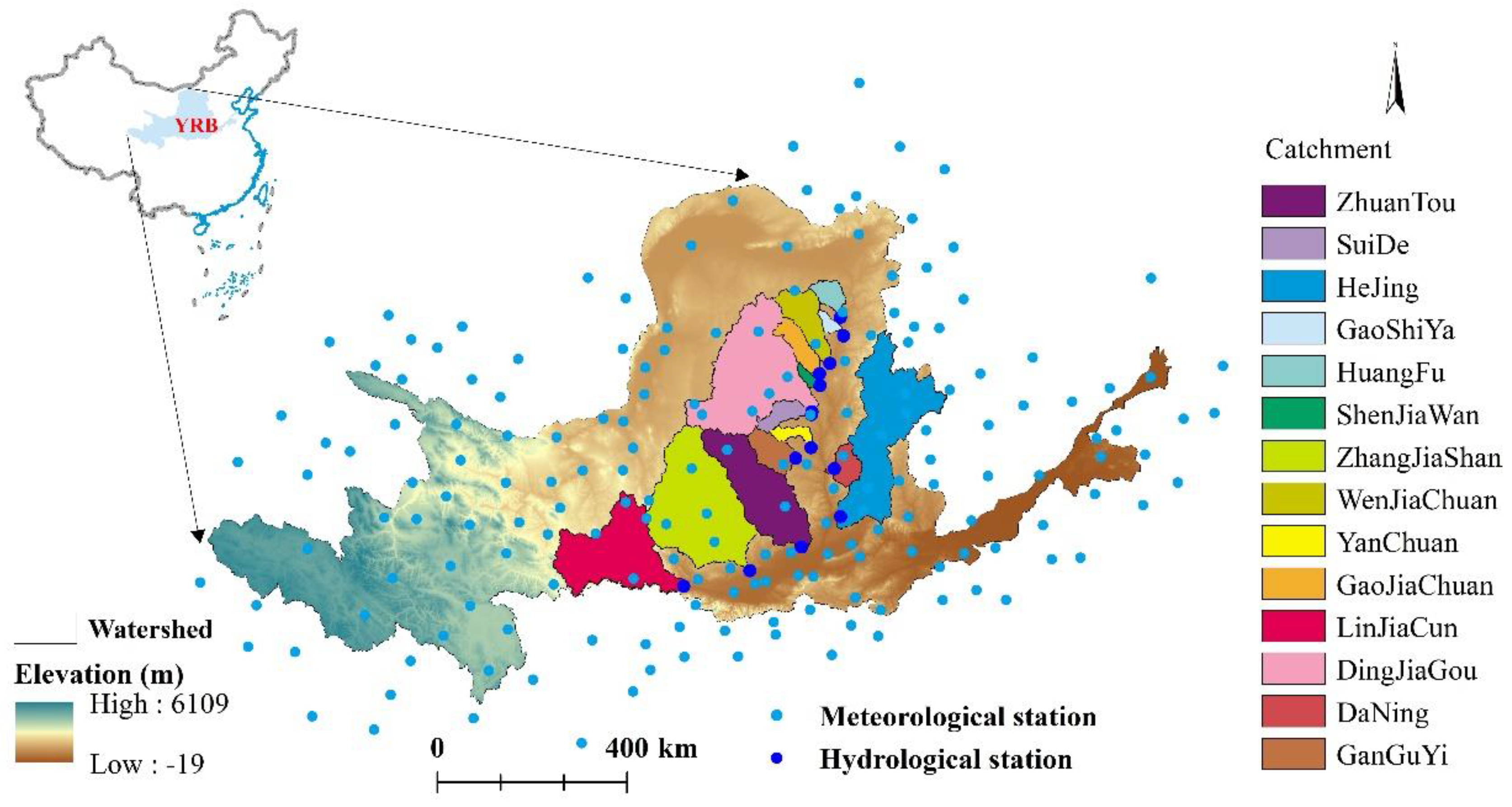
2.1. Study Area

The Yellow River is the main source of water in northwestern and northern China. The YRB, a semiarid basin, is located between 95°E–119°E and 32°N–42°N, covering an area of approximately 7.95 × 10⁵ km² (Figure 1). The annual precipitation ranges from 140 mm yr⁻¹ in the north to 1100 mm yr⁻¹ in the east of the YRB, with an average value of 495.6 mm yr⁻¹. Precipitation is concentrated in the summer months. The irrigation agriculture is developed, and there are four major irrigation areas along the Yellow River. In the midstream of the region, the ecological environment is fragile and land degradation is severe [43]. A series of ecological restoration projects have been implemented, such as nature reserves, the Three-North Shelterbelt, and the Grain to Green Program, of which the area covered by the Grain to Green Program is the largest among all of the ecological restoration programs [44].

2.2. Data Sources

2.2.1. MODIS Data

Sixteen-day interval normalized vegetation index (NDVI) images (MOD13A2 and MYD13A2 version 6 (V6) products) and 8-day interval land surface temperature (LST) images (MOD11A2 and MYD11A2 version6 (V6) products) with a spatial resolution of 1 km covering the whole YRB were downloaded from the Level-1 and Atmosphere Archive & Distribution System (LAADS) Distributed Active Archive Center (DAAC) website (https://ladsweb.modaps.eosdis.nasa.gov/). MOD11A2 and MOD13A2 were produced from the Aqua satellite images during the years 2003–2015, while MYD11A2 and MYD13A2 were produced from Terra satellite images during the years 2003–2015. To simplify processing, we defaulted the 16-day NDVI values in MOD13A2 and MYD13A2, which occur in the median day. Over the short time period, there are small changes in NDVI. “Day of year VI pixel” provides the date of the NDVI value, which appears within 16 days. Therefore, we can avoid large errors by setting the date when the 16-day interval NDVI value appears in the middle, and do not use “day of year VI pixel”. “Quality reliability of VI pixel” provides the quality of the pixel. In time series, we first used the Savitzky–Golay filtering to process the 23-period NDVI to obtain a new NDVI time series. For the new NDVI time series, we replaced the pixel values of the corresponding positions in the new time series with the high-quality pixel values of the original time series. The time resolution doubling algorithm [45] was used to fuse MOD13A2 and MYD13A2 during the years 2003–2015 to produce 8-day interval NDVI products. The missing values in MOD11A2 and MYD11A2 were filled by the adaptive window method [46], which constructs the relationship between the valid LST and NDVI, temperature, and elevation ($\mathrm{LST}~\mathrm{NDVI}+\mathrm{Temperature}+\mathrm{elevation}$), and uses the relationship to calculate the no data values in LST.

2.2.2. Meteorological Data

Daily meteorological data, including the atmospheric pressure (pa), temperature (°C) at a height of 2m (maximum temperature (°C), minimum temperature (°C)and mean temperature (°C)), wind speed (m s⁻¹) at a height of 10 m, sunshine hours (hour), and relative humidity (%) from 2003 to 2015, were collected from the website of the National Meteorological Administration of China (http://data.cma.cn). The daily meteorological data were subjected to a good quality control via the website of the National Meteorological Administration of China. The quality control method includes: (1) valid range check; (2) extreme inspection of stations; (3) internal consistency check between the timing value, daily average value, and daily extreme value; (4) time consistency check; and (5) spatial consistency check. The total meteorological station number of sites is 163, distributed inside and around the YRB (Figure 1). The daily weather data were aggregated into an 8-day interval weather dataset using an averaging method. Combining climatologic and topographic data, the point climate data were interpolated at a 1-km resolution covering the whole YRB, using the thin-plate smoothing spline method provided in the ANUSPLIN 3.1 program [47,48,49]. The interpolated climate raster data were used to calculate reference evapotranspiration by the Penman-Monteith equation [50].

2.2.3. ET Products

Given the scale of the basins in this paper, eight ET products with spatial resolutions higher than 0.1° (listed in

Table 1. Basic information about each evapotranspiration (ET) product.

Name	Time Period	Method	Resolution	Data Source
ETMTE	1982–2015	Upscaling	0.1°/month	Li et al. 2018
ETCR	1982–2015	CR	0.1°/month	http://www.tpedatabase.cn
ETMODIS	2001–2019	RS-PM	500 m/8 days	https://modis.gsfc.nasa.gov/data/dataprod/mod16.php
ETSSEBopGlo	2003–2019	SEB	1 km/month	https://earlywarning.usgs.gov/
ETBESS	2001–2015	RS-PM	1 km/8 days	http://environment.snu.ac.kr/
ETSEBS	2001–2016	SEB	0.05°/day	http://www.tpedatabase.cn
ETGLASS	2001–2015	BMA	0.05°/8 days	http://www.geodata.cn
ETPMLV2	2002–2018	RS-PM	0.05°/8 days	http://www.tpdc.ac.cn/

Note: MTE = model tree ensemble. BESS = breathing earth system simulator. SEBS = surface energy balance system. GLASS = Global Land-Surface Satellite. PMLV2 = Penman–Monteith –Leuning model version 2. SEB = surface energy balance. CR = complementary relationship. RS = remote sensing. PM = Penman–Monteith equation. BMA = Bayesian model average. ET = evapotranspiration.

) were collected to compare with ET_SSEBopYRB. The algorithms used to produce eight ET products cover the mainstream ET estimation methods. The information about the time period, spatial resolution, data source, and spatial coverage of each ET product is listed in Table 1. Since the common time period for the ET products selected in this paper was 2003–2015, we took 2003–2015 as the time period for ET evaluation.

The ET_MTE is a china ET product that is produced by the upscaling method of a model tree ensemble with four kinds of data inputs: (1) remote sensing data of NDVI 3 g; (2) the eddy covariance technique observing ET data at 36 sites covering forest, shrub-land, grassland, wetland, and cropland; (3) the climate data for surface air temperature, precipitation, incoming solar radiation, and relative humidity; and (4) the vegetation distribution map [34]. The validation results showed that this product can capture ET well for nine different vegetation types. Compared with the global data-driven ET product [12], this product is less uncertain in China due to the use of more China flux tower data.

The ET_CR is the China ET product that is estimated using the calibration-free nonlinear complementary relationship (CR) model, with climate variables (air and dew-point temperatures at a height of 2 m, wind speed at a height of 10 m, downward shortwave and downward longwave solar radiation) and remote sensing data (monthly land surface temperature, longwave broadband emissivity, and land surface albedo from MODIS) inputs [51]. Validation results from the 13 eddy covariance measurements and water-balance-derived ET for 10 major river basins showed that this product was reliable in China [51].

The ET_MODIS is the global ET product that is based on the Penman–Monteith equation [52]. It is composed of information for the vegetation transpiration, soil evaporation, and evaporation from the wet canopy surface. The data inputs of ET_MODIS are land cover (MOD12Q1), FPAR/Leaf area index (MOD15A2H), albedo (MOD43C1), and global Modern-Era Retrospective Analysis for Research and Applications (MERRA) meteorological data provided by the NASA Global Modeling and Assimilation Office (GMAO). This product has been applied in many regions [2,53]. Some studies have reported the shortcomings of ET_MODIS, such as underestimating the ET of farmland [31,54].

The ET_BESS is the global ET product that is produced using the simplified process-based model of the breathing earth system simulator (BESS), which can couple atmosphere and canopy radiative transfers, photosynthesis, and ET. The BESS adopts a quadratic form of the Penman–Monteith (PM) equation to calculate the two-leaf canopy latent heat flux [6]. Seven MODIS atmosphere (collection 6 MOD04_L2 aerosol, MOD06_L2 cloud, and MOD07_L2 atmosphere profile) and land (collection 5 MCD12Q1, MOD11A1, MOD06_L2, MCD15A2, and MCD43B3) products, four other satellite datasets, four reanalysis datasets, and three ancillary datasets were the input data for ET_BESS. At the site scale, ET_BESS agreed with FLUXNET observations, with R² = 0.67, and captured the majority of the seasonal variability [55].

ET_PMLV2 is the global ET product that is based on the Penman–Monteith –Leuning model version 2. The main focus of the PM-based method is the accurate estimation of surface conductance (Gs), which describes the canopy–soil conductance to the water flux. Leuning et al. (2008) [56] and Zhang et al. (2010) [57] developed the biophysical model for Gs to account for canopy physiological processes and soil evaporation (resulting in PMLv1). Gan et al. (2018) [58] coupled vegetation transpiration with gross primary productivity using a biophysical canopy conductance (Gc) model in the PML model (resulting in PMLv2). Zhang et al. applied the PMlv2 model [59] at the global scale with 0.25° resolution and 3-h Global Land Data Assimilation System (GLDAS-2.1 meteorological data, monthly atmospheric (CO2) concentration, LAI (MCD15A3H), albedo (MCD43A3), and surface emissivity data (MOD11A2) inputs. The ET_PMLV2 method is well-calibrated against 8-day EC ET at 95 widely distributed flux towers for ten plant functional types [59].

Two global ET products based on the surface energy balance method were released by Senay et al. (2013) [17] and Chen et al. (2019) [60]. The former is based on the SSEBop model (hereafter ET_SSEBopGlo) with the inputs of model-assimilated weather datasets and MODIS thermal images, while the latter is based on the surface energy balance system (hereafter ET_SEBS) with a column canopy–air turbulent diffusion method [60].

Considering that a single process-based algorithm cannot characterize global ET well, the Bayesian model averaging method was used to merge five process-based algorithms (hereafter ET_GLASS), including the MODIS latent heat flux product algorithm, the revised remote-sensing-based PM LE algorithm [61], the Priestley–Taylor-based LE algorithm [62], the modified satellite-based Priestley-Taylor LE algorithm [63], and the semiempirical Penman LE algorithm [64], to reduce the ET estimate uncertainty [65]. The production process of ET_GLASS is based on the Global Land-Surface Satellite (GLASS) data.

2.2.4. Regional Database for ET Model Evaluation

Annual ET evaluation data from 2003 to 2015 were derived from the water balance approach (annual ET is the difference in annual precipitation and annual streamflow, ignoring the soil water storage change). Because the streamflow of the fourteen catchments (Figure 1) is dominated by surface runoff, annual changes of soil water and groundwater are not likely to be large [39]. Therefore, ignoring the soil water storage change does not cause large water balance ET uncertainly in these catchments. Water balance ET (hereafter WB-ET) is an ordinary practice and a reliable method used to estimate basin-scale ET when streamflow and precipitation are accessible [10]. The annual streamflow of each hydrological site came from the Chinese Annual Hydrographic Yearbook of the Yellow River Basin (http://www.mwr.gov.cn/). The information on the 14 hydrological sites (total 182 samples) used for ET evaluation is listed in

Table 2. Hydrological characteristics of catchments for model validation.

Hydrological Station	Station Location	Catchment Area (km2)	Annual Runoff (108 m3)	Annual Precipitation (mm)
DaNing	110.71 E, 36.46 N	4186	0.84	514
DingJiaGou	110.25 E, 37.55 N	41948	6.70	339
GanGuYi	109.8 E, 36.7 N	5857	1.51	482
GaoJiaChuan	110.48 E, 35.56 N	4955	2.14	378
GaoShiYa	111.13 E, 38.93 N	1260	0.18	399
Hejing	110.8 E, 35.56 N	39186	5.07	486
HuangFu	111.08 E, 39.28 N	3230	0.36	375
ShenJiaWan	110.48 E, 38.03 N	1138	0.33	405
SuiDe	110.23 E, 37.5 N	3861	1.07	416
WenJiaChuan	110.75 E, 38.43 N	8621	2.17	373
YanChuan	110.18 E, 36.8 N	2095	0.98	458
ZhangJiaShan	108.6 E, 34.63 N	43106	10.32	484
ZhuangTou	109.83 E, 35.03 N	25645	0.21	519

. The spatial distribution of the sites and the watershed extent are shown in Figure 1. The watershed boundaries are from previous studies [39,66]. The annual precipitation dataset was produced using ANUSPLIN3.1 to interpolate 507 precipitation points within and around the YRB (Figure A4). In addition, we also collected three other precipitation datasets, including Tropical Rainfall Measuring Mission satellite precipitation data (TRMM3b42), which were derived from remote sensing satellite [67], reanalysis data of Climatic Research Unit (CRU) [68], as well as the precipitation product of the China meteorological forcing dataset (CMFD) [69], in order to analyze the uncertainty of WB-ET.

2.3. Methods

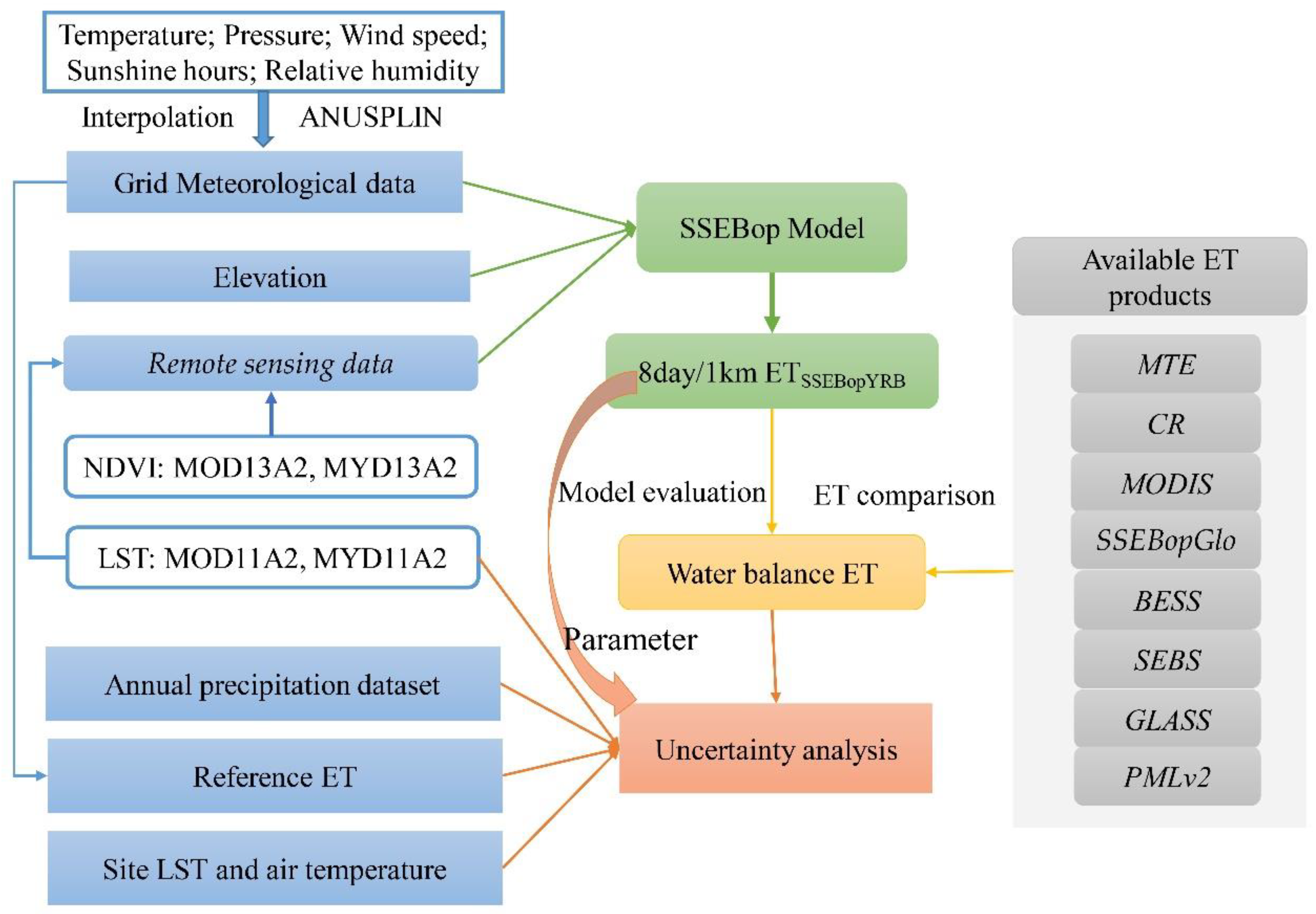
2.3.1. Framework of the Assessment of ET_SSEBopYRB

Figure 2 shows the framework for evaluating ET_SSEBopYRB, which includes the input and output of the SSEBop model, evaluation of ET_SSEBopYRB with water balance ET, comparison between ET_SSEBopYRB and available eight ET products, and the uncertainty analysis of ET_SSEBopYRB.

2.3.2. SSEBop Model

In previous surface energy balance methods (e.g., SEBAL), the ET is the residual of the energy balance terms ($\mathsf{\lambda }\mathrm{ET}=R_n-H-G$, where H is the sensible heat (MJ m⁻² day⁻¹), G is the soil heat (MJ m⁻² day⁻¹), Rn is the net radiation (MJ m⁻² day⁻¹), and $\mathsf{\lambda }$is the latent heat of evaporation of water). Among the four variables, the calculation process of H is complicated and especially depends on the setting of cold pixels and hot pixels. The SSEBop model assumes that the surface energy balance process is mostly driven by the available net radiation (Rn), and a decline in ET due to water stress and other factors can be quantified by differences in land surface temperature [8]. SSEBop directly estimates pixel-based ET by multiplying the ET fraction ($E{T}_f$) and reference ET ($E{T}_o$).

$${ET}_a={ET}_f\times k_{mas}\times {ET}_o$$

(1)

where $k_{max}$ is a coefficient that scales the grass reference ET into the level of a maximum ET experienced by an aerodynamically rougher crop; $E{T}_o$ is the grass reference ET (mm day⁻¹), which is calculated using the revised PM equation in YRB [50,70].

$$E{T}_o=\left[0.408\Delta \left(R_n-G\right)+\gamma \frac{900}{Tem+273}{u}_{2}VPD\right]/\left[\mathsf{\Delta }+\gamma \left(1+0.34u_2\right)\right]$$

(2)

where $\Delta$is the slope of the vapor pressure curve (kPa °C ⁻¹), $\gamma$is the psychrometric constant (kPa °C ⁻¹),$Tem$is the mean daily air temperature (°C) at a height of 2 m, $u_2$ is the wind speed at a height of 2 m (m s⁻¹), and $VPD$is the water vapor pressure difference (kPa).$E{T}_f$ is calculated as follows:

$$E{T}_f=\left[\left(T_h-T_s\right)/\left(T_h-T_c\right)\right]$$

(3)

where T_s is the eight-day average satellite-observed LST of the pixel (K), T_h is the estimated $T_s$ at the idealized reference “hot–dry” limit of the same pixel for the same time period, and $T_c$ is the estimated T_s at the idealized “cold–wet” limit of the same pixel. The minimum ET_f is set to 0.09, the maximum ET_f is 1.05, and the $E{T}_f$ exceeding 1.3 is considered to be a pixel with cloud pollution and is set to “no data”. The “no data” is filled through temporal interpolation [17]:

$$T_c=c\times T_a$$

(4)

$$\mathrm{c}=\left(T_{s\_cold}/T_a\right)$$

(5)

where $T_a$ is the eight-day average near-surface maximum air temperature (K), $c$ is a correction factor that relates $T_a$ to $T_{s\_cold}$; $T_{s\_cold}$ is the eight-day average LST on a well-watered, fully transpiring vegetation surface; $T_{s\_cold}$ is obtained on all pixels where NDVI is greater than or equal to 0.8. If no pixels in an image in a certain period meet the NDVI conditions, the $c$ value of that image is the median value of the effective $c$ value within one year:

$$T_h=T_c+dT$$

(6)

where $dT$ is a predefined temperature difference (K) between $T_h$ and $T_c$ for each pixel. The minimum value of $dT$ is recommended as 6 K, which can reduce the ET uncertainty in cold climates [17]:

$$\mathrm{dT}=\left(R_{n,cs}\times r_{ah}\right)/\left({\rho }_a\times C_p\right)$$

(7)

where $r_{ah}$ is the aerodynamic resistance to heat flow from a hypothetical bare and dry surface (110 s m⁻¹), ${\rho }_a$ is the air density (kg m⁻³), $C_p$ is the specific heat of the air at constant pressure (~1.013 kJ kg⁻¹K⁻¹), and $R_{n,cs}$ is the clear-sky net radiation (MJ m⁻² day⁻¹), which is estimated using the series of equations in [50]:

$$R_{n,cs}=R_{ns}-R_{nl}$$

(8)

$$R_{ns}=\left(1-\alpha \right)\times R_s$$

(9)

$$R_s=(0.75+2\times {10}^{-5}\times z)R_a$$

(10)

$$R_{nl}=\sigma \times \left(\frac{T_{max}{}^4+T_{min}{}^4}{2}\right)\times \left(0.34-0.14\sqrt{ea}\right)$$

(11)

where $R_{ns}$ and $R_{nl}$ are the clear sky net shortwave radiation (MJ m⁻² day⁻¹) and clear sky longwave radiation (MJ m⁻² day⁻¹); $\alpha$ is the surface albedo, which is set to 0.23 in this study; $R_s$ and R_a are the clear sky incoming solar radiation (MJ m⁻² day⁻¹) and extraterrestrial radiation (MJ m⁻² day⁻¹); z is the elevation (m); $\sigma$is the Stefan–Boltzmann constant (4.9039 10⁻⁹ MJ K⁻⁴ m⁻²day_-1). $T_{max}$ and $T_{min}$ are the air maximum and minimum temperatures (K), and $ea$ is the actual vapor pressure (kPa). More details about $R_a$ and $ea$ can be found in [50].

The difference between the SSEBop model and other energy balance models is that it predefines a differential temperature ($dT$) as two extreme limiting surface temperatures—a cold temperature ($T_c$) for little or no sensible heat flux and hot temperature ($T_h$) for little or no latent heat flux, eliminating the subjectivity that could be introduced during manual hot and cold reference selection. More detailed information about the calculation process for SSEBop can be found in [8,17]. This study mainly used MOD11A2 and climate datasets to drive the SSEBop model to estimate the ET of the YRB.

2.3.3. Trend Analysis

We conducted linear regression based on the least squares method to detect the trend for annual ET. The regression coefficient was used as the annual ET change rate:

$$\mathrm{b}=\frac{{{\displaystyle \sum }}_{i=1}^{13}\left(E{T}_i-\overline{ET}\right)\left(y_i-\overline{y}\right)}{{{\displaystyle \sum }}_{i=1}^{13}{\left(E{T}_{yi}-\overline{ET}\right)}^2}$$

(12)

where i is the sequential year range (2003–2015), ET_i is the annual ET in the year y_i, and $\overline{ET}$ and $\overline{y}$ are the mean values. A positive or negative value predicts an increased or decreased rate of annual water yield. If the regression coefficient passes through the significance test (F test, p < 0.05), it shows a significant ascending or descending trend [71,72].

2.3.4. Performance of Estimated ET

Commonly used hydrological model evaluation metrics such as the coefficient of determination (R²), root mean square error (RMSE), and relative percent error ($\mathrm{RPE}$) [13] are used in this paper. The formula of$\mathrm{RPE}$is as follows:

$$\mathrm{RPE}=\left[\left(X-Y\right)/Y\right]\times 100$$

(13)

where X is the simulated ET and Y is the observed ET. The closer the RPE (%) is to 0, the smaller the difference between the average of the observed and simulated values.

3. Results

3.1. Evaluation of SSEBopYRB-ET on a Basin Scale

ET_SSEBopYRB’s estimated annual ET performance for 14 small watersheds was lower than ET_SSEBopGlo from the RMSE (88.30 mm yr⁻¹ vs. 82.59 mm yr⁻¹) and R² (0.49 vs. 0.52) values (Figure 3). ET_SSEBopGlo overestimated 3.01% of the annual WB-ET, while ET_SSEBopYRB underestimated 3.38% of the annual WB-ET. Compared with the ET_SEBS, ET_MODIS, ET_CR, and ET_GLASS, ET_SSEBopYRB had better performance when estimating the annual WB-ET, with a higher R², lower RMSE, and lower absolute RPE. ET_MODIS, ET_SEBS, and ET_CR highly underestimated the annual WB-ET, with RPE values of –19.97%, −28.73%, and −26.54%, respectively, while ET_GLASS highly overestimated annual WB-ET (44.59%). As a widely used product, ET_MODIS could only explain 37% of the annual WB-ET variability and had a much higher RMSE (121.75 mm yr⁻¹ vs. 88.30 mm yr⁻¹) than ET_SSEBopYRB. ET_MTE and ET_PMLV2 had lower RMSE values than ET_SSEBopYRB, but had smaller R² and higher absolute RPE values than ET_SSEBopYRB. ET_BESS had a lower RMSE (79.01 mm yr⁻¹ vs. 88.30 mm yr⁻¹) than ET_SSEBopYRB, but ET_BESS underestimated 11.62% of the annual WB-ET.

We also evaluated ET_SSEBopYRB and the other eight ET products from the perspective of the multiyear average ET using the multiyear average WB-ET on 14 small watersheds (total 14 samples). The result showed that ET_SSEBopYRB performed better than six (ET_SEBS, ET_SSEBopGlo, ET_GLASS, ET_CR, ET_MODIS, and ET_MTE) out of the eight ET products (

Table 3. Evaluation of average annual ET during the years 2003–2015.

ET Product	R2	RMSE (mm yr−1)	RPE (%)
ETSEBS	0.95	125.32	−28.73
ETBESS	0.87	54.02	−11.62
ETSSEBopYRB	0.85	60.09	−3.38
ETSSEBopGlo	0.84	63.25	3.01
ETGLASS	0.79	224.73	44.59
ETCR	0.70	120.38	−26.54
ETPMLv2	0.69	44.00	5.28
ETMODIS	0.65	105.45	−19.97
ETMTE	0.17	58.31	−4.11

). The R², RMSE, and RPE values for ET_SSEBopYRB were 0.85, 60.09 mm yr-1, and −3.38%, respectively, indicating that there is good agreement between ET_SSEBopYRB and WB-ET on a multiyear scale. The R² of ET_SSEBopYRB was slightly lower than that of ET_BESS (0.87 vs. 0.85), but the RPE for ET_BESS was higher than for ET_SSEBopYRB. Although the RMSE for ET_PMLv2 was lower than ET_SSEBopYRB, ET_PMLv2 could only explain 69% of the WB-ET variability, which was lower than ET_SSEBopYRB.

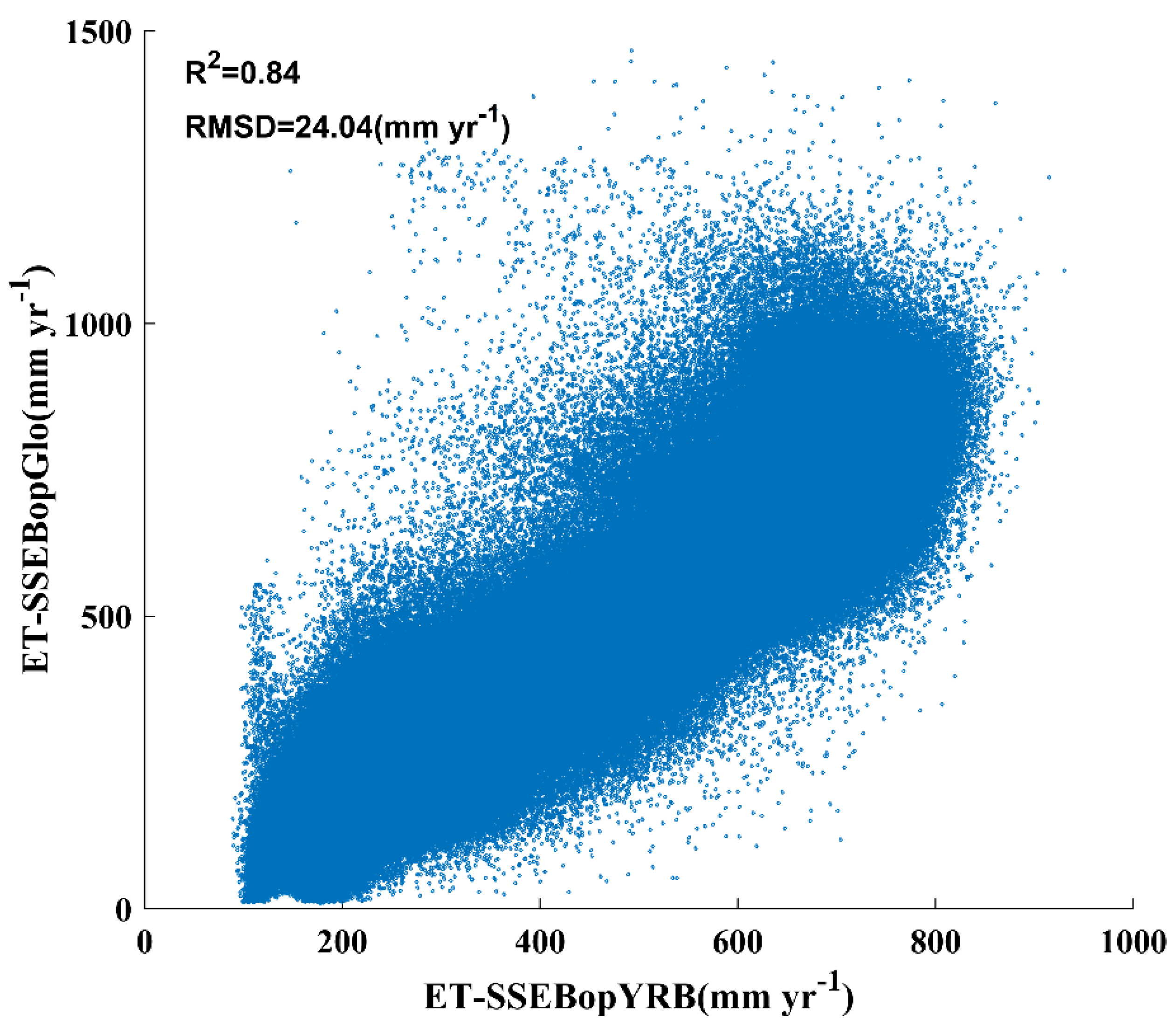
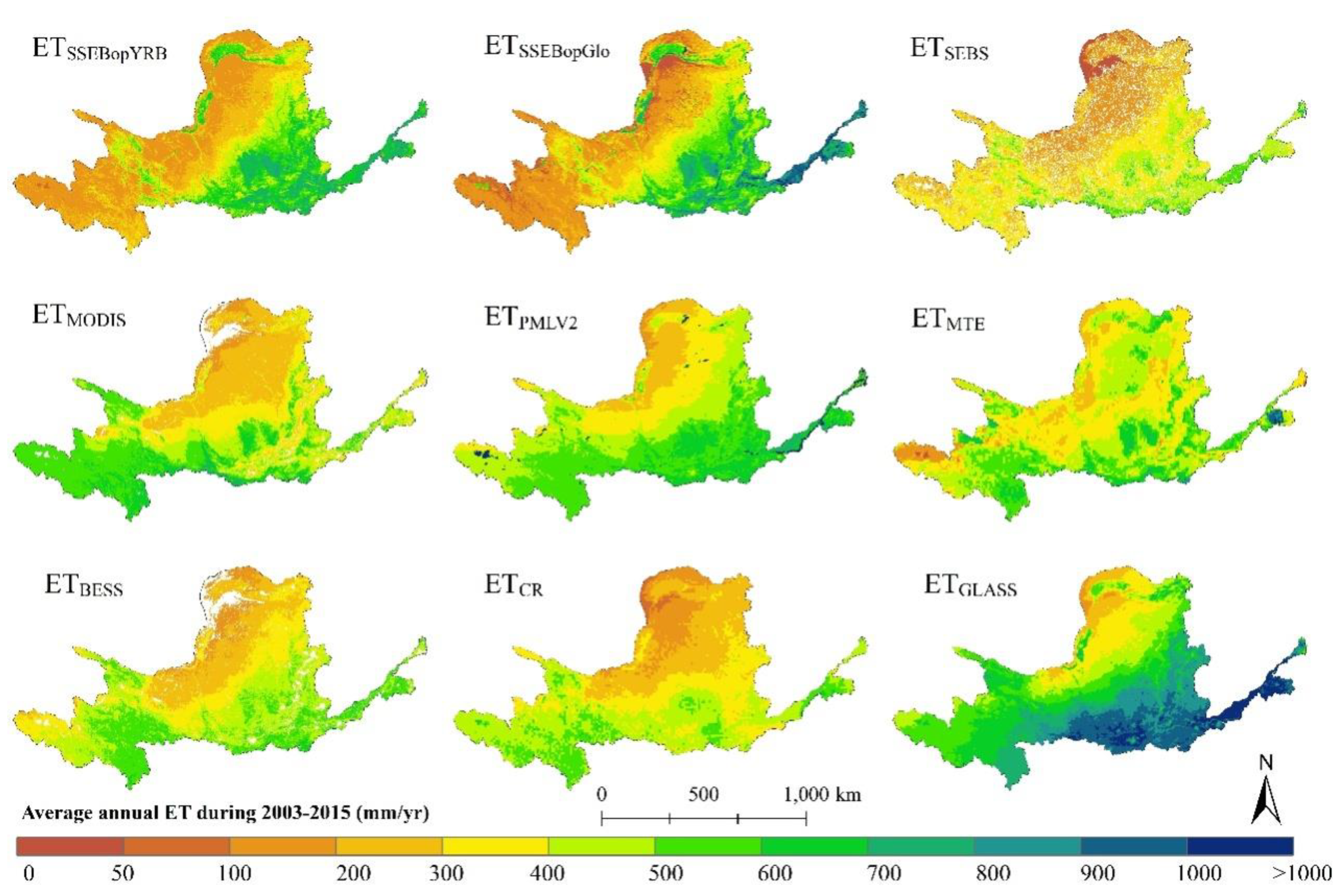
3.2. Spatial Pattern Comparison between ETSSEBopYRB and Other ET Products

The spatial pattern of the average annual ET_SSEBopYRB during 2003–2015 in YRB exhibited a notable high value in the east and low value in the west (Figure 4), which is similar to the findings for ET_SSEBopGlo. The main difference between ET_SSEBopYRB and the other seven ET products was concentrated on the upper YRB and irrigated farmland. In the upper YRB, the mean annual ET estimated by ET_SSEBopYRB and ET_SSEBopGlo ranged from 200 to 300 mm yr⁻¹, while the estimated mean annual ET of the other seven ET products was higher than that of ET_SSEBopYRB. For example, ET_MODIS ranged from 600 to 700 mm yr⁻¹, while the ET_CR ranged from 400 to 600 mm yr⁻¹ in the upper YRB (Figure 4). In the irrigated farmland located in the north (Figure A1), the mean annual ET values for ET_SSEBopYRB, ET_SSEBopGlo, and ET_GLASS ranged from 500 to 700 mm yr⁻¹, while the mean annual ET values estimated by the other six ET products ranged from 200 to 500 mm yr⁻¹.

Averaged over all vegetated areas (all land cover types except the barren type reported in Figure A1), the YRB mean annual ET_SSEBopYRB weighted by area during the years 2003–2015 was 369.26 ± 29.72 mm yr⁻¹, which included 84.04% ± 8.27% of the mean annual precipitation (Figure 5). This result was slightly higher than those of ET_SEBS and ET_CR and slightly lower than those of ET_SSEBopGlo (375.63 mm yr⁻¹) and ET_BESS (395.32 mm yr⁻¹). The mean annual ET estimates for the YRB in the ET_MTE, ET_PMLV2, and ET_GLASS were higher than that in the ET_SSEBopYRB and larger than the mean annual precipitation. Considering that the main land type in the YRB is grassland (Figure A1), it is impossible for the average annual average ET to exceed the average annual precipitation. On a multiyear scale (e.g., 13 years), ignoring changes in groundwater in the YRB, the average annual ET of YRB derived from the water balance method using the run-off data from the Water Resources Bulletin of the YRB (http://www.yrcc.gov.cn/) is 375.86 mm. Therefore, ET_MTE, ET_PMLV2, and ET_GLASS highly overestimated the mean annual ET of the YRB, while the annual average ET of YRB estimated by ET_SSEBopYRB was reasonable.

3.3. Trend Comparison between ETSSEBopYRB and other ET Products

Figure 6 shows that the annual ET trend in the YRB estimated by ET_SSEBopYRB shows an increasing trend in most areas (75.24%), of which the increase in the central part is more obvious, while the increase in the western part is lower. In the western YRB, the annual ET values in ET_SSEBopYRB and ET_SEBS mainly decreased, which is different from ET_SSEBopYRB. In the irrigated farmland located in the north of the YRB, the annual ET in ET_SSEBopYRB decreased, while the annual ET for other ET products increased. In the central parts of the YRB where the NDVI increased significantly (Figure A2), all ET products showed that the annual ET increased. In the south of the YRB, the annual ET for ET_SSEBopYRB decreased, which was similar to ET_SSEBopGlo, ET_CR, and ET_GLASS and different from ET_MODIS, ET_PMLV2, and ET_BESS.

Overall, the annual ET of the YRB simulated by ET_SSEBopYRB during 2003–2015 showed a significantly increased trend with a slope of 4.34 mm yr⁻¹, which was lower than the annual ET trends from ET_MODIS and ET_PMLV2 and higher than the annual ET trends from the other six ET products (

Table 4. Annual ET trend statistics for the whole YRB during the years 2003–2015.

ET Product	ET Slope (mm yr−1)	Significant Increase (%)	Significant Decrease (%)	Non-Significant Increase (%)	Non-Significant Decrease (%)
ETMODIS	6.61 *	58.16	0.72	37.90	3.21
ETPMLv2	5.16 *	53.50	0.36	43.53	2.60
ETSSEBopYRB	4.34 *	12.74	1.16	62.50	23.60
ETMTE	3.35 *	35.28	1.19	45.47	18.07
ETGLASS	1.78	16.88	5.83	55.19	22.10
ETBESS	1.59	22.21	4.43	45.67	27.69
ETCR	1.24	12.00	1.19	50.38	36.43
ETSSEBopGlo	0.92	9.30	5.85	44.02	40.83
ETSEBS	-1.05	2.63	11.03	31.07	55.26

Note: * means the p-value is below 0.05.

). The annual rate for ET change for the whole YRB estimated by ET_SSEBopGlo was only 0.92 mm yr⁻¹, which was much lower than that of the ET_SSEBopYRB. The reason for the different trends between ET_SSEBopGlo and ET_SSEBopYRB is that the forcing climate data are different. The annual ET trend type for ET_SSEBopYRB is mainly a non-significant increase with a proportion of 62.50%, while the annual ET trend type for ET_SSEBopGlo is mainly a non-significant increase (44.02%) and non-significant decrease (40.83%).

4. Discussion

The annual total ET trend in the YRB showed a significant increase for ET_SSEBopYRB but no significant change for ET_SSEBopGlo. When researchers directly apply the free global ET product simulated by SSEBop, especially the ET trend analysis, validation should be done if possible. In cases of flux data unavailability, the water balance method could be used or ET products could be compared with global ET products in their research area. Some researchers directly applied this product to analyze the relationships between ET variability and vegetation dynamics without validating the reliability of the product in the Nile Basin, Africa [26,27]. To further improve the estimation of ET, the uncertainty of ET_SSEBopYRB in this research area should be discussed.

4.1. The Effect of Potential ET Estimation on ET Uncertainty

The reference ET is one of the most sensitive factors in the SSEBop model [32]. In this paper, we use the PM formula [50] to calculate the reference ET with the eight-day average pressure, sunshine hours, wind speed, relative humidity, minimum temperature, maximum temperature, and mean temperature as inputs. The optimal interpolation method for each climate variable is different [73], but each climate variable was interpolated using the same thin-plate spline function interpolation method, which may cause reference errors and affect the ET. Because the reference ET is strongly related to the pan evaporation [50], the small observed pan evaporation in the station within the YRB from 2003 to 2015 was used to evaluate the reference ET. The results showed that the correlation coefficient of the eight-day average reference ET and small pan evaporation ranged from 0.86 to 0.95 (Figure 7), which indicated a strong relationship between the reference ET and the small pan evaporation. In the earlier research, three different methods, including the standard global PM formula [50], revised PM formula in China [74], and the revised PM formula in the YRB [70], were used to calculate the reference ET in the YRB. The difference between the three methods focuses on the radiation term. The difference in the annual reference ET of the YRB simulated by the three methods is very small (Figure A3). Therefore, the uncertainty of the reference ET in this research cannot cause the large ET uncertainty simulated by the SSEBop model in the YRB from 2003 to 2015.

4.2. Influence of the Land Surface Temperature Product on ET Uncertainty

The errors of LST images (MOD11A2) are generally within ±1 K in most areas, especially in the areas that have complicated biophysical conditions, or arid or semiarid climatic conditions, which contain errors of up to ±5 K [75]. The YRB is a typical arid and semiarid river basin, which results in large uncertainty in the LST. An uncertainty assessment of the SSEBop model implemented in the United States showed that an error of LST within a range of 0.35% (i.e., ±1 K) can lead to an ET error in the range of 20% [32]. We used the observed LST data from 94 meteorological stations evenly distributed across the YRB (Figure A6) and air temperature to evaluate MOD11A2 and MYD11A2 during the years 2003–2015.

The 8-day average satellite LST, including MYD11A2 and MOD11A2, in the YRB can explain 92–96% of the 8-day average site LST during the years 2003–2014, except 2015 (Figure 8). The LST curve for MOD11A2 was abnormal in 2015, however MYD11A2 was not. The abnormal 8-day average MOD11A2 LST curves in 2015 were different from the eight-day LST curves in 2000–2014 throughout the YRB and on the meteorological observation sites, while the eight-day average observed LST curve and eight-day average observed air mean temperature curve were normal in 2015 (Figure 8). We assumed that the above phenomenon was due to the large missing values in MOD11A2 in 2015. However, after performing statistical analysis of the missing MOD11A2 ratio for the whole YRB and meteorological observation sites, we found that our assumption was wrong, because the missing ratio in 2015 was the same as the missing ratio during the years 2003–2014 (Figure A7). We concluded that the MOD11A2 product could not characterize the YRB’s eight-day average LST variability in 2015.

Obviously, abnormal LST decreases the accuracy of the ET_f and then decreases the accuracy of ET according to the principles of the SSEBop model. We also ran the SSEBop model with the MYD11A2 input to calculate the 8-day interval ET in the YRB during the years 2003–2015. Figure A8 shows that the eight-day average YRB ET_f derived from MYD11A2 (hereafter ETf_MYD) and the eight-day average YRB ETf from MOD11A2 (hereafter ETf_MOD) were inconsistent for days 137–153 and days 297–337 in 2015. The abnormal LST of MOD11A2 in 2015 occurs during days 137–153 and days 169–217. Although there were abnormal MOD11A2 LST values for days 169–217, the ETf_MOD value was normal and the same as ETf_MYD, which is related to the ET_f temporal interpolation method. The ET_f temporal interpolation method had no effect on days 169–217 in 2015. Correspondingly, the intrayear change of the average YRB ET derived from MYD11A2 (hereafter ET_{SSEBopYRB, MYD}) was very close to the ET_SSEBopYRB, which was derived from MOD11A2 during the years 2003–2014, except for 2015 at the 8-day scale and monthly scale (Figure A9 and Figure A10). This is closely related with the intrayear change of the eight-day ET_f. The abnormal ET_SSEBopYRB value in 2015 occurred on days 137–153 at the eight-day scale and in May at the monthly scale. The 8-day LST abnormal data for MOD11A2 had a weak influence on the YRB annual ET (Figure A11). Therefore, abnormal eight-day LST data have a great influence on the intravariability of ET, but have a small influence on the interannual variability.

It should be noted that due to the scale mismatch between in situ measurements and satellite-based observations, it is relatively difficult to obtain true values for pixels, especially for terrestrial regions that are typically heterogeneous and non-isothermal terrestrial regions [76]. Figure A7 shows that the average missing LST value ratio (average of 46 ratios of missing LST values per year) in each image varies from 2.22% to 5.04% during the years 2003–2015. However, the missing LST ratio for some of the dates is as high as 25% or more (Figure A7). The filling method for the LST missing value causes different errors [46]. This paper adopted the adaptive window method, which considers the relationship between high-quality pixel LST values and influencing factors (e.g., elevation, NDVI, and air temperature) to fill the missing values [77].

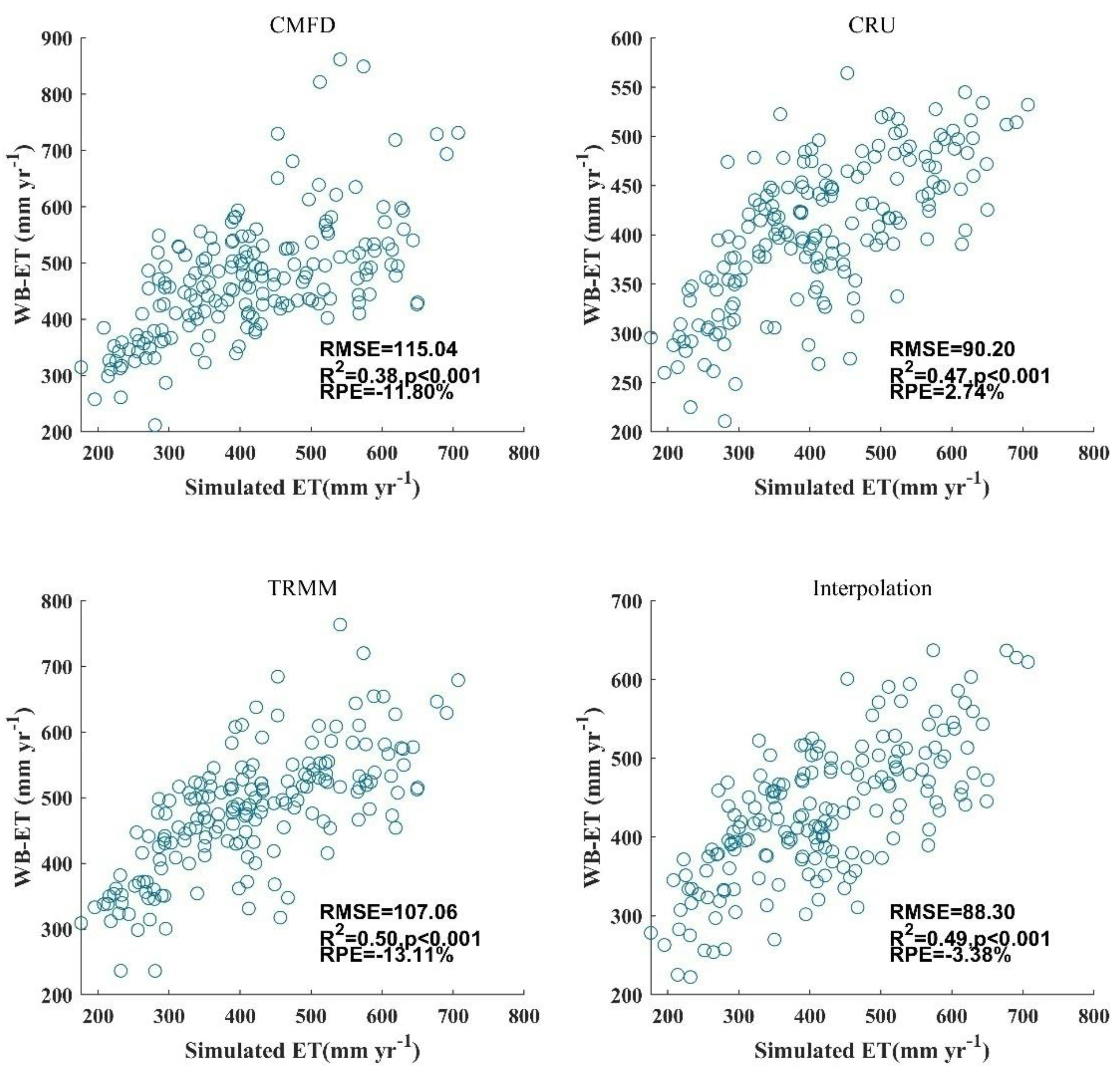
4.3. Influence of Precipitation Products on ET Uncertainty

This paper used the difference between annual precipitation and run-off (WB-ET) as the annual evaluation data for ET_SSEBopYRB. The uncertainty of the precipitation and run-off was approximately 10% for the water-balanced ET method [78]. Compared to the YRB precipitation site interpolation involved in previous studies [39,79], the annual precipitation was interpolated using more rain gauge stations (N = 507 vs. N = 134) (Figure A4). With more site distributions, the annual precipitation uncertainty caused by the different interpolation methods, the thin-plate spline function, ordinary kriging, and inverse distance weight was small (Figure A5). Cross validation results indicated that interpolated precipitation using the three methods accounted for 84.1% ± 1.7% of the annual precipitation observed at the sites (Figure A5). The unexplained 15% may be due to the complexity of the land surface in the YRB, which greatly increases the interpolation difficulty.

There are also some free global coarse resolution precipitation products, such as TRMM3b42 derived from remote sensing satellites [67] and reanalysis data of CRU [68], while the Chinese precipitation product from the China meteorological forcing dataset (CMFD) integrates ground observations, satellite data, and reanalysis data [80]. ET_SSEBopYRB can explain 38%, 47%, 50%, and 49% of the WB-ET based on the CMFD, CRU, TRMM3b42, and the interpolation of the annual precipitation, respectively, during the years 2003–2015. In the \ RMSE and RPE indices, there were lower RMSE and lower RPE values for WB-ET based on interpolation than for WB-ET based on the other three precipitation products (Figure 9). Therefore, the WB-ET used for evaluation will have a great impact on the evaluation results because of the differences in annual precipitation data.

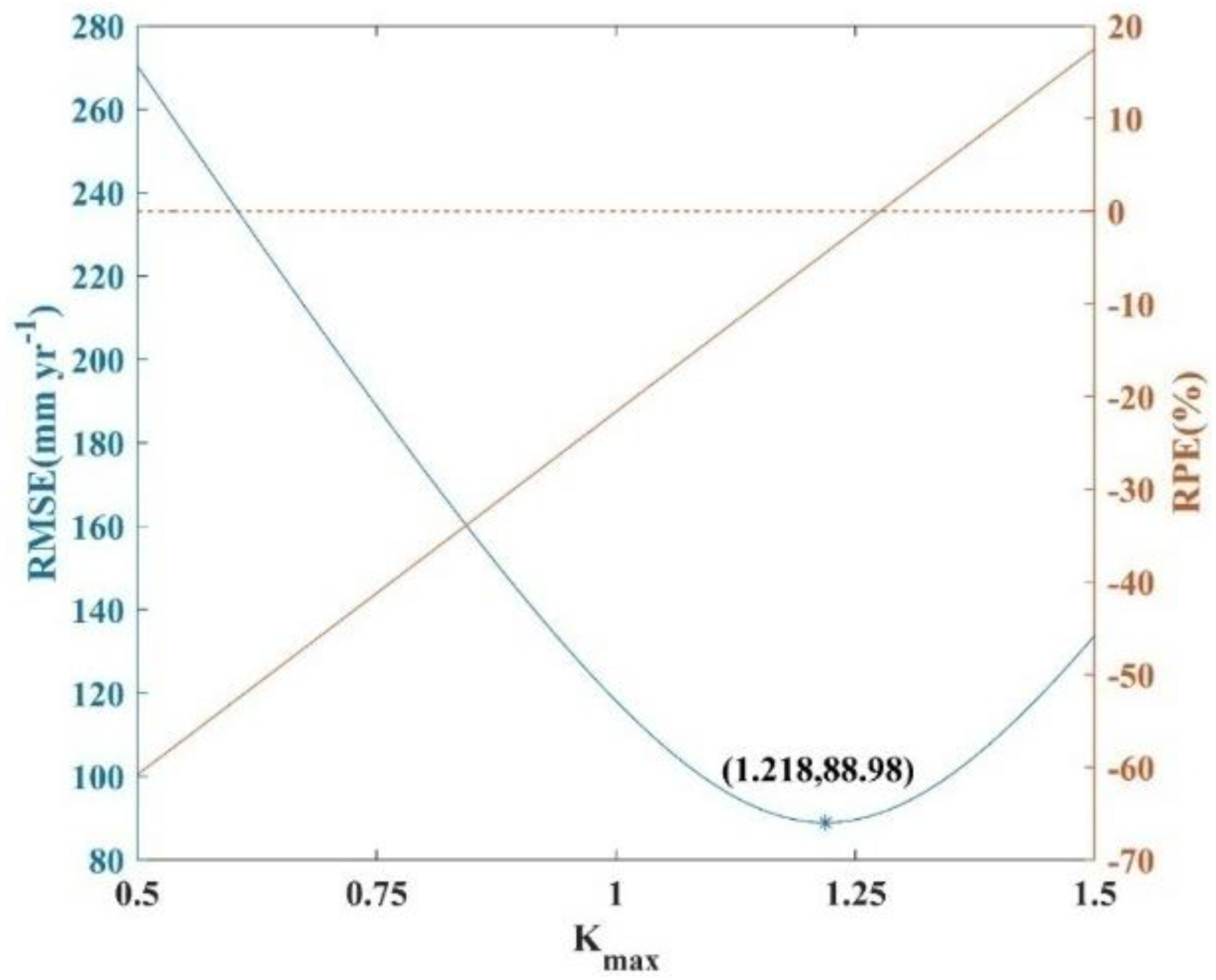
4.4. Influence of Model Parameters on ET Uncertainty

The model parameters of coefficient $k_{max}$ involving the magnitude of the estimated ET are additional sensitive and critical factors in the SSEBop model [32]. The coefficient $k_{max}$ factor was recommended to be set at 1.2 in the original research [8]. Later, Chen et al. (2016) recommended that the coefficient $k_{max}$ range should be from 0.95 to 1.2, and that it was acceptable to take the coefficient $k_{max}$ as 1.1, since its maximum error of 15% leads to an ET uncertainty of approximately 15% [32]. Senay et al. (2018) highly emphasized the correction of this factor in the applied research region using the WB-ET or site observation ET [17]. In this research, through the correction using WB-ET in 2003–2014, the coefficient $k_{max}$ was set as 1.218 (Figure 10). When the coefficient $k_{max}$ was 1.2168, the RMSE (88.98 mmyr⁻¹) between the WB-ET and ET_SSEBopYRB (the LST input is MOD11A1) during the years 2003–2014 was lower than the other f $k_{max}$ setting, while the RPE (−4.49%) for ET_SSEBopYRB was small.

4.5. Influence of the Basin Size on ET Uncertainty

The fourteen basins have different basin sizes, varying from 1138 km² to 43,106 km², which may influence the evaluation results. According to whether a watershed’s area is larger or smaller than 10,000 km², the 14 small watersheds were divided into two groups. The evaluation of the large basins (Figure A12) showed that the nine ET products could only explain 22–63% of the ET variability. For all ET products except ET_MTE, the simulated ET could explain higher ET variability than if all fourteen basins were included, especially for ET_SEBS (0.43 vs. 0.59), ET_CR (0.41 vs. 0.54), ET_GLASS (0.40 vs. 0.54), and ET_PMLv2 (0.41 vs. 0.62). The improvements of R² values for ET_SSEBopYRB (0.49vs. 0.51) and ET_SSEBopGlo were relatively small (0.52 vs. 0.57). RMSE values also changed, especially for ET_MODIS and ET_GLASS. ET_MODIS and ET_GLASS in the five large area basins had much lower (121.75 mm yr⁻¹ vs. 84.50 mm yr⁻¹) and higher (232.12 mm yr⁻¹ vs. 307.35 mm yr⁻¹) RMSE values, respectively, than that for all fourteen basins. The increases in RMSE values for ET_SSEBopYRB (88.30 mm yr⁻¹ vs. 96.65 mm yr⁻¹) and ET_SSEBopGlo (82.59 mm yr⁻¹ vs. 84.66 mm yr⁻¹) were small. In terms of the RPE, the changes for ET_SSEBopYRB and ET_SSEBopGlo were low, but were high in ET_MODIS (−19.97% vs. −5.83%). Therefore, the basin size did not have a great impact on the evaluation of ET_SSEBopYRB and ET_SSEBopGlo, but did have a noticeable influence on the evaluation of ET_MODIS.

4.6. Difference between ET_SSEBopYRB and Eight Other ET Products

The results section showed the differences between the ET_SSEBopYRB and the eight other ET products in capturing the annual ET for fourteen small catchments (Figure 3, Table 3), estimating the average annual ET in YRB (Figure 4), and simulating the ET trend for the YRB (Figure 5, Table 4).

ET_SSEBopYRB and ET_SSEBopGlo are both driven by the SSEBop model, however with different input datasets. A scatter plot based on the pixel values of the mean annual ET values shows that the R² is as high as 0.84 and the root mean square difference (RMSD) is as low as 24.04 mm yr⁻¹ (Figure A13). The small differences in the spatial distribution of the mean annual ET for the YRB during the years 2003–2015 are related to the same forcing data as MOD11A2 being used, the same methods (PM equation) being used to calculate the reference ET, and the same method (temporal interpolation) being used to interpolate the no data value for ET_f. The differences in the ET trends for the YRB are mainly due to the differences in the reference ET trends. The meteorological data used to calculate the reference ET for ET_SSEBopGlo are derived from GLDAS, while the meteorological data used for ET_SSEBopYRB were interpolated using regional dense station data.

The differences between ET_SSEBopYRB and the other seven ET products are not just driven by model physics, but also forcing data. The forcing datasets for each ET product are described in Section 2.2.3. Eight-day MODIS LST and 16-day NDVI values are the main inputs used to quantify the land surface conditions in ET_SSEBopYRB. The ET products that had similar remote sensing input data to ET_SSEBopYRB were ET_SEBS, ET_CR, ET_BESS, ET_MTE, and ET_GLASS. The daily MODIS LST, eight-day MODIS LST. and monthly MODIS LST were the important inputs for ET_SEBS, ETBESS, and ET_CR, respectively. ET_MTE and ET_GLASS used GIMMS NDVI and MODIS NDVI to represent land surface conditions, respectively. The ET products that had different remote sensing input data for ET_SSEBopYRB were ET_MODIS and ET_PMLv2. ET_MODIS and ET_PMLv2 used the eight-day MODIS LAI and FPAR data to characterize the land surface conditions. There was a correlation between NDVI and LAI-FPAR.

In terms of the meteorological forcing data, many ET products (e.g., ET_MODIS) rely upon global reanalysis data, which have their limitations. For example, Modern Era Retrospective Analysis for Research and Applications- meteorological data provided by the NASA Global Modeling and Assimilation Office, which has a spatial resolution of 1/2° × 2/3°, uses the same meteorological data as in ET_MODIS and ET_GLASS. ET_BESS adopts National Centers for Environmental Prediction (NCEP)/National Center for Atmospheric Research (NCAR) reanalysis data, while ET_PMLv2 adopts the 0.25° resolution and 3-h GLDAS-2.1 data. ET_CR and ET_MTE both use the 0.1° CMFD data as the meteorological forcing data. The trend differences among these various climate datasets in the YRB affect the estimated ET trend.

5. Conclusions

We conducted a comparison of ET values derived from the SSEBop model using the water balance ET values in a highly spatially heterogeneous river basin (the YRB) and reached the following conclusions for the years 2003–2015:

(1)

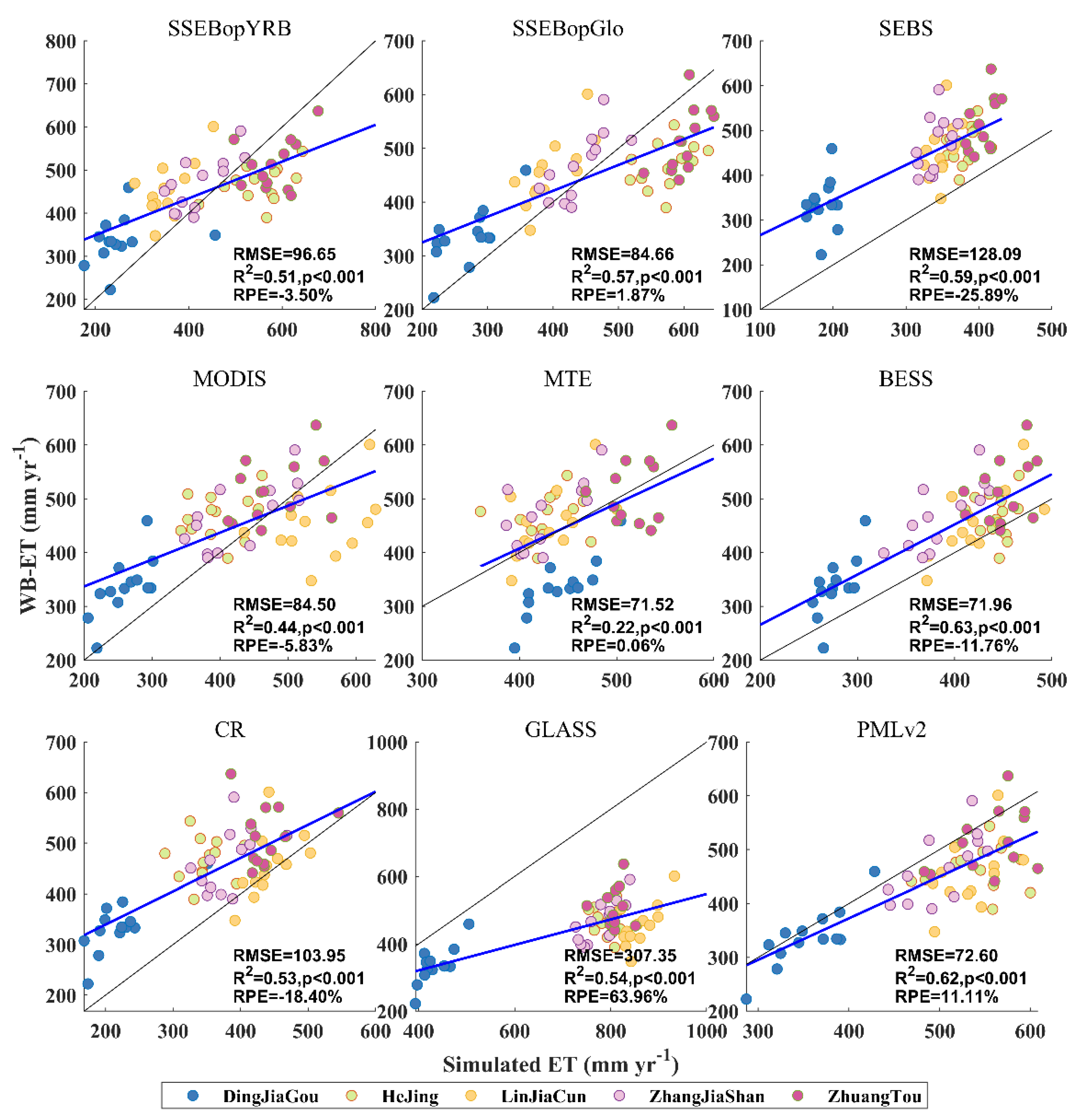
ET_SSEBopYRB and the other eight ET products were able to explain 23 to 52% of the variability in WB-ET for fourteen small catchments in YRB. ET_SSEBopYRB had better agreement with WB-ET than ET_SEBS, ET_MODIS, ET_CR, and ET_GLASS, with lower RMSE (88.3 mm yr⁻¹ vs. 121.7 mm yr⁻¹), higher R² (0.49 vs. 0.43), and lower absolute RPE (−3.3% vs. −19.9%) values;

(2)

The free global ET product derived from the SSEBop model highly underestimated the annual total ET trend for the YRB. More validation regarding this product is required in other regions using site measurements (e.g., eddy covariance flux tower measurements);

(3)

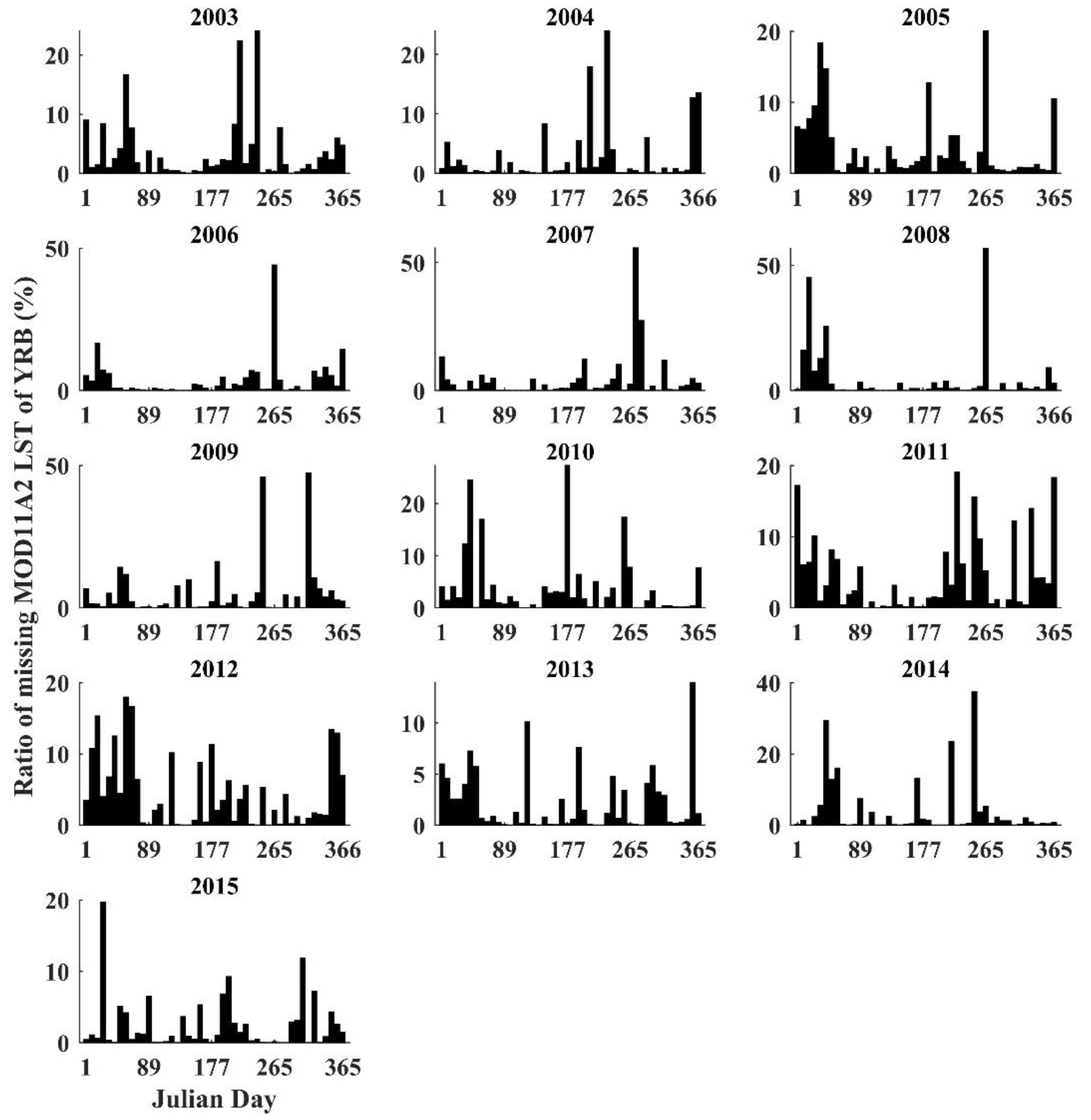
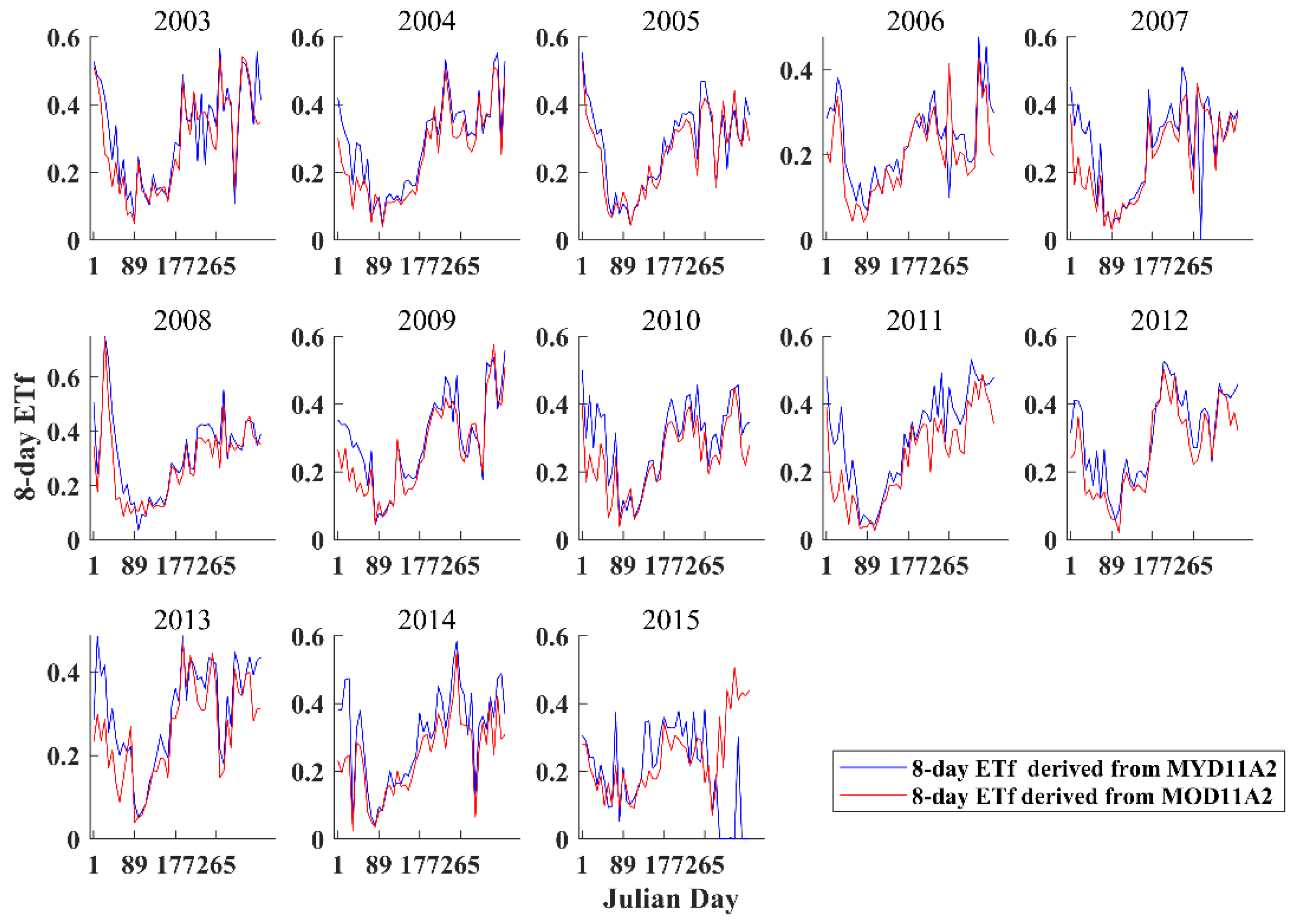
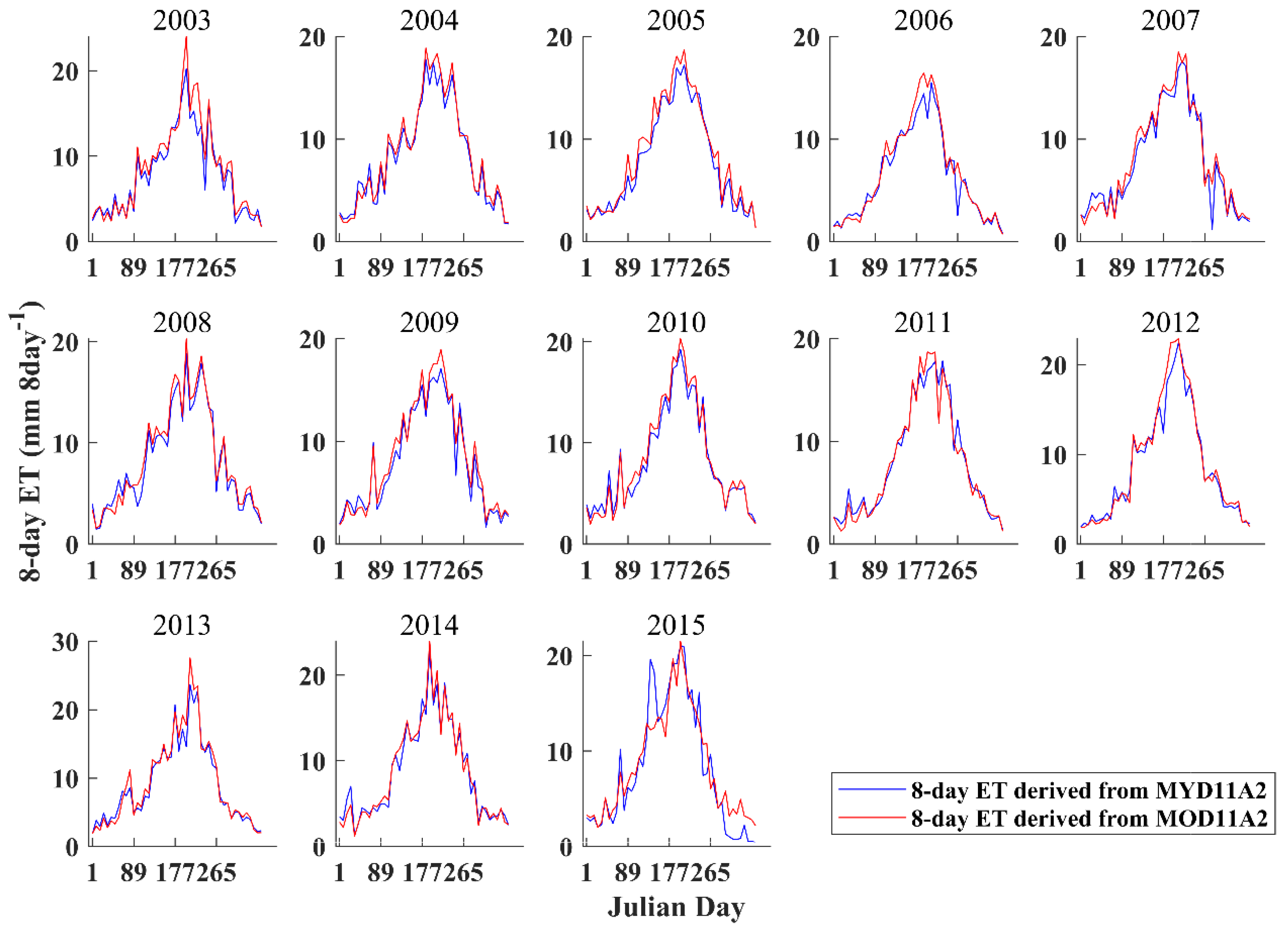
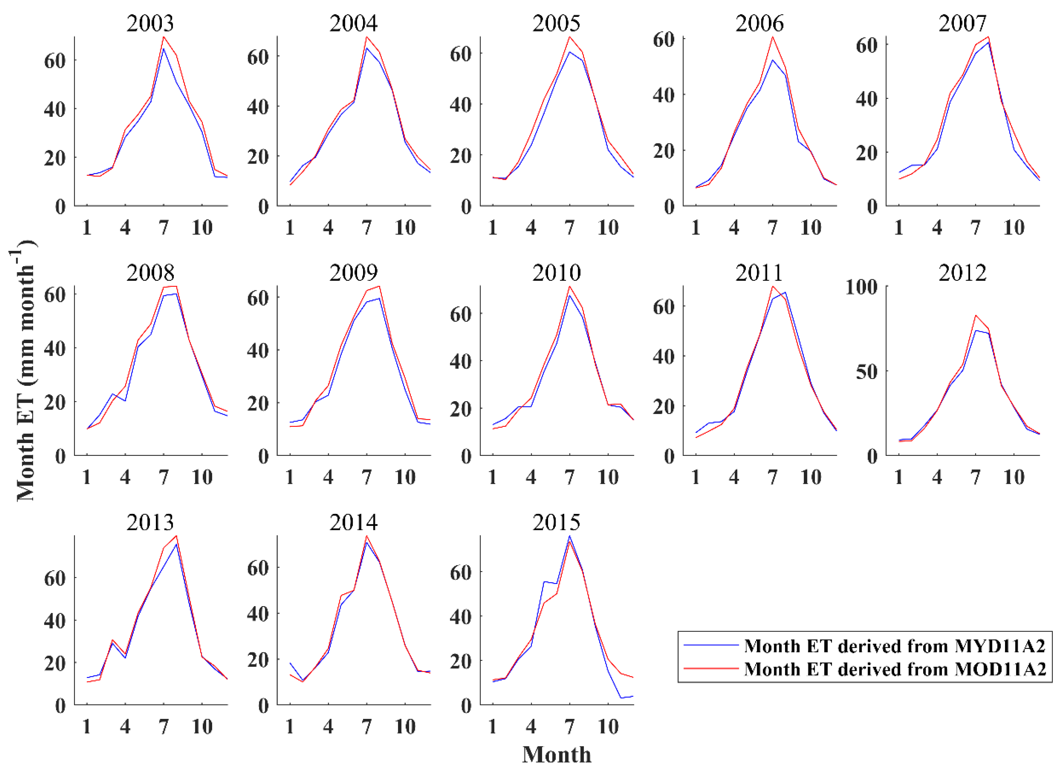
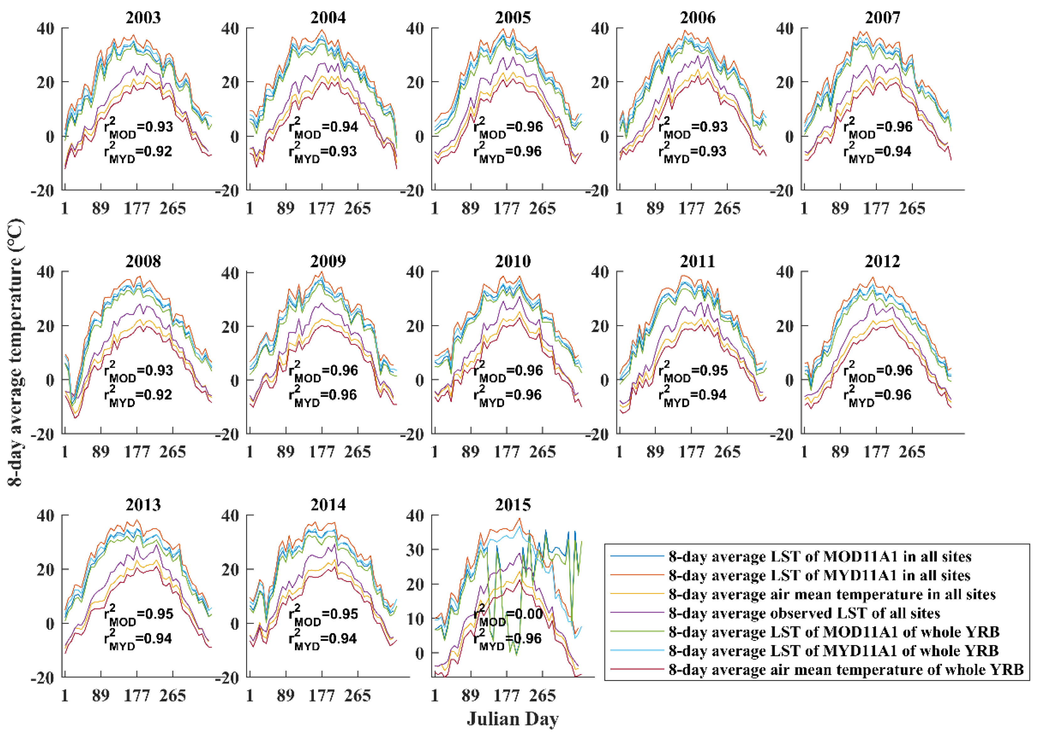
The abnormal data in the land surface temperature products of MOD11A2 for 2015 limited the performance of the SSEBop model at the eight-day and monthly scales. Future studies will explore the use of MYD11A2;

(4)

At the basin scale, the uncertainties of the ET trends and spatial patterns are still large for different ET products. We need to further reduce the ET uncertainty to better serve water resource management and ecological restoration project construction purposes.

References

1. Baldocchi, D.; Dralle, D.; Jiang, C.; Ryu, Y. How Much Water Is Evaporated Across California? A Multiyear Assessment Using a Biophysical Model Forced with Satellite Remote Sensing Data. Water Resour. Res. 2019, 55, 2722–2741. [Google Scholar] [CrossRef]
2. Feng, X.; Fu, B.; Piao, S.; Wang, S.; Ciais, P.; Zeng, Z.; Lü, Y.-H.; Zeng, Y.; Li, Y.; Jiang, X.; et al. Revegetation in China’s Loess Plateau is approaching sustainable water resource limits. Nat. Clim. Chang. 2016, 6, 1019–1022. [Google Scholar] [CrossRef]
3. Zhang, M.; Wang, S.; Fu, B.; Gao, G.; Shen, Q. Ecological effects and potential risks of the water diversion project in the Heihe River Basin. Sci. Total. Environ. 2018, 619, 794–803. [Google Scholar] [CrossRef] [PubMed]
4. Feng, X.M.; Liu, Q.L.; Yin, L.C.; Fu, B.J.; Chen, Y.Z. Linking water research with the sustainability of the human-natural system. Curr. Opin. Environ. Sustain. 2018, 33, 99–103. [Google Scholar]
5. Sun, G.; Alstad, K.; Chen, J.; Chen, S.; Ford, C.R.; Lin, G.; Liu, C.; Lu, N.; McNulty, S.G.; Miao, H.; et al. A general predictive model for estimating monthly ecosystem evapotranspiration. Ecohydrology 2010, 4, 245–255. [Google Scholar] [CrossRef]
6. Ryu, Y.; Baldocchi, D.; Kobayashi, H.; Van Ingen, C.; Li, J.; Black, T.A.; Beringer, J.; Van Gorsel, E.; Knohl, A.; Law, B.; et al. Integration of MODIS land and atmosphere products with a coupled-process model to estimate gross primary productivity and evapotranspiration from 1 km to global scales. Glob. Biogeochem. Cycles 2011, 25, 25. [Google Scholar] [CrossRef] [Green Version]
7. Hu, Z.; Li, S.; Yu, G.-R.; Sun, X.; Zhang, L.; Han, S.; Li, Y. Modeling evapotranspiration by combing a two-source model, a leaf stomatal model, and a light-use efficiency model. J. Hydrol. 2013, 501, 186–192. [Google Scholar] [CrossRef]
8. Senay, G.B.; Bohms, S.; Singh, R.; Gowda, P.H.; Velpuri, M.; Alemu, H.; Verdin, J.P. Operational Evapotranspiration Mapping Using Remote Sensing and Weather Datasets: A New Parameterization for the SSEB Approach. JAWRA J. Am. Water Resour. Assoc. 2013, 49, 577–591. [Google Scholar] [CrossRef] [Green Version]
9. Liu, Z.; Yao, Z.; Wang, R. Simulation and evaluation of actual evapotranspiration based on inverse hydrological modeling at a basin scale. Catena 2019, 180, 160–168. [Google Scholar] [CrossRef]
10. Palmroth, S.; Katul, G.; Hui, D.; McCarthy, H.R.; Jackson, R.B.; Oren, R. Estimation of long-term basin scale evapotranspiration from streamflow time series. Water Resour. Res. 2010, 46, 46. [Google Scholar] [CrossRef] [Green Version]
11. Wang, K.; Wang, P.; Li, Z.; Cribb, M.; Sparrow, M. A simple method to estimate actual evapotranspiration from a combination of net radiation, vegetation index, and temperature. J. Geophys. Res. Space Phys. 2007, 112, 112. [Google Scholar] [CrossRef]
12. Jung, M.; Reichstein, M.; Ciais, P.; Seneviratne, S.I.; Sheffield, J.; Goulden, M.L.; Bonan, G.; Cescatti, A.; Chen, J.; De Jeu, R.; et al. Recent decline in the global land evapotranspiration trend due to limited moisture supply. Nature 2010, 467, 951–954. [Google Scholar] [CrossRef]
13. Bhattarai, N.; Mallick, K.; Stuart, J.; Vishwakarma, B.D.; Niraula, R.; Sen, S.; Jain, M. An automated multi-model evapotranspiration mapping framework using remotely sensed and reanalysis data. Remote Sens. Environ. 2019, 229, 69–92. [Google Scholar] [CrossRef]
14. Roerink, G.; Su, Z.; Menenti, M. S-SEBI: A simple remote sensing algorithm to estimate the surface energy balance. Phys. Chem. Earth Part B Hydrol. Oceans Atmos. 2000, 25, 147–157. [Google Scholar] [CrossRef]
15. Yang, Y.; Shang, S.; Jiang, L. Remote sensing temporal and spatial patterns of evapotranspiration and the responses to water management in a large irrigation district of North China. Agric. For. Meteorol. 2012, 164, 112–122. [Google Scholar] [CrossRef]
16. Chen, X.; Su, Z.; Ma, Y.; Liu, S.; Yu, Q.; Xu, Z. Development of a 10-year (2001–2010) 0.1° data set of land-surface energy balance for mainland China. Atmos. Chem. Phys. Discuss. 2014, 14, 13097–13117. [Google Scholar] [CrossRef] [Green Version]
17. Senay, G.B. Satellite Psychrometric Formulation of the Operational Simplified Surface Energy Balance (SSEBop) Model for Quantifying and Mapping Evapotranspiration. Appl. Eng. Agric. 2018, 34, 555–566. [Google Scholar] [CrossRef] [Green Version]
18. Lopes, J.D.; Rodrigues, L.N.; Imbuzeiro, H.M.A.; Pruski, F.F. Performance of SSEBop model for estimating wheat actual evapotranspiration in the Brazilian Savannah region. Int. J. Remote Sens. 2019, 40, 6930–6947. [Google Scholar] [CrossRef]
19. De Paula, A.C.P.; De Figueiredo, C.C.; Rodrigues, L.N.; Warren, M.S. Performance of the SSEBop model in the estimation of the actual evapotranspiration of soybean and bean crops. Pesquisa Agropecuária Brasileira 2019, 54, 54. [Google Scholar] [CrossRef]
20. Wagle, P.; Bhattarai, N.; Gowda, P.H.; Zhou, Y. Performance of five surface energy balance models for estimating daily evapotranspiration in high biomass sorghum. ISPRS J. Photogramm. Remote Sens. 2017, 128, 192–203. [Google Scholar] [CrossRef] [Green Version]
21. Velpuri, N.M.; Senay, G.B. Partitioning Evapotranspiration into Green and Blue Water Sources in the Conterminous United States. Sci. Rep. 2017, 7, 6191. [Google Scholar] [CrossRef] [PubMed]
22. Bhattarai, N.; Wagle, P.; Gowda, P.H.; Zhou, Y. Utility of remote sensing-based surface energy balance models to track water stress in rain-fed switchgrass under dry and wet conditions. ISPRS J. Photogramm. Remote Sens. 2017, 133, 128–141. [Google Scholar] [CrossRef]
23. Senay, G.B.; Schauer, M.; Friedrichs, M.; Velpuri, N.M.; Singh, R.K. Satellite-based water use dynamics using historical Landsat data (1984–2014) in the southwestern United States. Remote Sens. Environ. 2017, 202, 98–112. [Google Scholar] [CrossRef]
24. Singh, R.; Senay, G.B. Comparison of Four Different Energy Balance Models for Estimating Evapotranspiration in the Midwestern United States. Water 2015, 8, 9. [Google Scholar] [CrossRef] [Green Version]
25. Singh, R.; Senay, G.B.; Velpuri, N.M.; Bohms, S.; Scott, R.L.; Verdin, J.P. Actual Evapotranspiration (Water Use) Assessment of the Colorado River Basin at the Landsat Resolution Using the Operational Simplified Surface Energy Balance Model. Remote Sens. 2013, 6, 233–256. [Google Scholar] [CrossRef] [Green Version]
26. Alemu, H.; Senay, G.B.; Kaptué, A.T.; Kovalskyy, V. Evapotranspiration Variability and Its Association with Vegetation Dynamics in the Nile Basin, 2002–2011. Remote Sens. 2014, 6, 5885–5908. [Google Scholar] [CrossRef] [Green Version]
27. Alemu, H.; Kaptué, A.T.; Senay, G.B.; Wimberly, M.C.; Henebry, G. Evapotranspiration in the Nile Basin: Identifying Dynamics and Drivers, 2002–2011. Water 2015, 7, 4914–4931. [Google Scholar] [CrossRef]
28. Alemayehu, T.; Van Griensven, A.; Senay, G.B.; Bauwens, W. Evapotranspiration Mapping in a Heterogeneous Landscape Using Remote Sensing and Global Weather Datasets: Application to the Mara Basin, East Africa. Remote Sens. 2017, 9, 390. [Google Scholar] [CrossRef] [Green Version]
29. Olivera-Guerra, L.; Mattar, C.; Merlin, O.; Durán-Alarcón, C.; Artigas, A.S.-; Fuster, R. An operational method for the disaggregation of land surface temperature to estimate actual evapotranspiration in the arid region of Chile. ISPRS J. Photogramm. Remote Sens. 2017, 128, 170–181. [Google Scholar] [CrossRef] [Green Version]
30. Tadesse, T.; Senay, G.B.; Berhan, G.; Regassa, T.; Beyene, S. Evaluating a satellite-based seasonal evapotranspiration product and identifying its relationship with other satellite-derived products and crop yield: A case study for Ethiopia. Int. J. Appl. Earth Obs. Geoinform. 2015, 40, 39–54. [Google Scholar] [CrossRef] [Green Version]
31. Velpuri, N.M.; Senay, G.; Singh, R.K.; Bohms, S.; Verdin, J. A comprehensive evaluation of two MODIS evapotranspiration products over the conterminous United States: Using point and gridded FLUXNET and water balance ET. Remote Sens. Environ. 2013, 139, 35–49. [Google Scholar] [CrossRef]
32. Chen, M.; Senay, G.B.; Singh, R.K.; Verdin, J.P. Uncertainty analysis of the Operational Simplified Surface Energy Balance (SSEBop) model at multiple flux tower sites. J. Hydrol. 2016, 536, 384–399. [Google Scholar] [CrossRef] [Green Version]
33. Bhattarai, N.; Shaw, S.B.; Quackenbush, L.; Im, J.; Niraula, R. Evaluating five remote sensing based single-source surface energy balance models for estimating daily evapotranspiration in a humid subtropical climate. Int. J. Appl. Earth Obs. Geoinform. 2016, 49, 75–86. [Google Scholar] [CrossRef]
34. Li, X.; He, Y.; Zeng, Z.; Lian, X.; Wang, X.; Du, M.; Jia, G.; Li, Y.; Ma, Y.; Tang, Y.; et al. Spatiotemporal pattern of terrestrial evapotranspiration in China during the past thirty years. Agric. For. Meteorol. 2018, 259, 131–140. [Google Scholar] [CrossRef]
35. Mueller, B.; Hirschi, M.; Jiménez, C.; Ciais, P.; Dirmeyer, P.A.; Dolman, H.; Fisher, J.; Jung, M.; Ludwig, F.; Maignan, F.; et al. Benchmark products for land evapotranspiration: LandFlux-EVAL multi-data set synthesis. Hydrol. Earth Syst. Sci. 2013, 17, 3707–3720. [Google Scholar] [CrossRef] [Green Version]
36. Jasechko, S.; Sharp, Z.D.; Gibson, J.J.; Birks, S.J.; Yi, Y.; Fawcett, P.J. Terrestrial water fluxes dominated by transpiration. Nature 2013, 496, 347–350. [Google Scholar] [CrossRef]
37. Xiong, Y.; Zhao, W.L.; Wang, P.; Paw U, K.T.; Qiu, G.Y. Simple and Applicable Method for Estimating Evapotranspiration and Its Components in Arid Regions. J. Geophys. Res. Atmos. 2019, 124, 9963–9982. [Google Scholar] [CrossRef]
38. Bai, M.; Mo, X.; Liu, S.; Hu, S. Contributions of climate change and vegetation greening to evapotranspiration trend in a typical hilly-gully basin on the Loess Plateau, China. Sci. Total Environ. 2019, 657, 325–339. [Google Scholar] [CrossRef]
39. Feng, X.M.; Sun, G.; Fu, B.J.; Su, C.H.; Liu, Y.; Lamparski, H. Regional effects of vegetation restoration on water yield across the Loess Plateau, China. Hydrol. Earth Syst. Sci. 2012, 16, 2617–2628. [Google Scholar] [CrossRef] [Green Version]
40. Xu, S.; Yu, Z.; Yang, C.; Ji, X.; Zhang, K. Trends in evapotranspiration and their responses to climate change and vegetation greening over the upper reaches of the Yellow River Basin. Agric. For. Meteorol. 2018, 263, 118–129. [Google Scholar] [CrossRef]
41. Yuan, X.; Bai, J. Future Projected Changes in Local Evapotranspiration Coupled with Temperature and Precipitation Variation. Sustainability 2018, 10, 3281. [Google Scholar] [CrossRef] [Green Version]
42. Fu, B.; Wang, S.; Liu, Y.; Liu, J.; Liang, W.; Miao, C. Hydrogeomorphic Ecosystem Responses to Natural and Anthropogenic Changes in the Loess Plateau of China. Annu. Rev. Earth Planet. Sci. 2017, 45, 223–243. [Google Scholar] [CrossRef]
43. Fu, B.; Liu, Y.; Lü, Y.; He, C.; Zeng, Y.; Wu, B. Assessing the soil erosion control service of ecosystems change in the Loess Plateau of China. Ecol. Complex. 2011, 8, 284–293. [Google Scholar] [CrossRef]
44. Lü, Y.; Fu, B.; Feng, X.; Zeng, Y.; Liu, Y.; Chang, R.; Sun, G.; Wu, B. A Policy-Driven Large Scale Ecological Restoration: Quantifying Ecosystem Services Changes in the Loess Plateau of China. PLoS ONE 2012, 7, e31782. [Google Scholar] [CrossRef] [PubMed]
45. Zhengxing, W.; Linghong, K.E.; Fangping, D. Doubling MODIS-NDVI Temporal Resolution: From 16-Day to 8-Day. Remote Sens. Technol. Appl. 2011, 26, 437–443. [Google Scholar]
46. Pede, T.; Mountrakis, G. An empirical comparison of interpolation methods for MODIS 8-day land surface temperature composites across the conterminous Unites States. ISPRS J. Photogramm. Remote Sens. 2018, 142, 137–150. [Google Scholar] [CrossRef]
47. Carter, C.; Liang, S. Comprehensive evaluation of empirical algorithms for estimating land surface evapotranspiration. Agric. For. Meteorol. 2018, 2018, 334–345. [Google Scholar] [CrossRef] [Green Version]
48. McVicar, T.R.; Van Niel, T.; Li, L.; Hutchinson, M.F.; Mu, X.; Liu, Z. Spatially distributing monthly reference evapotranspiration and pan evaporation considering topographic influences. J. Hydrol. 2007, 338, 196–220. [Google Scholar] [CrossRef]
49. Wahba, G.; Wendelberger, J.G. Some New Mathematical Methods for Variational Objective Analysis Using Splines and Cross Validation. Mon. Weather. Rev. 1980, 108, 1122–1143. [Google Scholar] [CrossRef] [Green Version]
50. Allen, R.G.; Pereira, L.S.; Raes, D.; Smith, M. Crop Evapotranspiration—Guidelines for Computing Crop Water Requirements-FAO Irrigation and drainage paper 56 1998. Available online: http://http://www.fao.org/3/X0490E/x0490e05.htm (accessed on 5 August 2020).
51. Ma, N.; Szilagyi, J.; Zhang, Y.; Liu, W. Complementary-Relationship-Based Modeling of Terrestrial Evapotranspiration across China during 1982–2012: Validations and Spatiotemporal Analyses. J. Geophys. Res. Atmos. 2019, 124, 4326–4351. [Google Scholar] [CrossRef]
52. Monteith, J.L. Evaporation and environment. Symp. Soc. Exp. Boil. 1965, 19, 205–234. [Google Scholar]
53. Peng, S.; Piao, S.; Zeng, Z.; Ciais, P.; Zhou, L.; Li, L.; Myneni, R.; Yin, Y.; Zeng, H. Afforestation in China cools local land surface temperature. Proc. Natl. Acad. Sci. USA 2014, 111, 2915–2919. [Google Scholar] [CrossRef] [PubMed] [Green Version]
54. Tang, R.; Shao, K.; Li, Z.-L.; Wu, H.; Tang, B.-H.; Zhou, G.; Zhang, L. Multiscale Validation of the 8-day MOD16 Evapotranspiration Product Using Flux Data Collected in China. IEEE J. Sel. Top. Appl. Earth Obs. Remote Sens. 2015, 8, 1478–1486. [Google Scholar] [CrossRef]
55. Jiang, C.; Ryu, Y. Multi-scale evaluation of global gross primary productivity and evapotranspiration products derived from Breathing Earth System Simulator (BESS). Remote Sens. Environ. 2016, 186, 528–547. [Google Scholar] [CrossRef]
56. Leuning, R.; Zhang, Y.; Rajaud, A.; Cleugh, H.; Tu, K. A simple surface conductance model to estimate regional evaporation using MODIS leaf area index and the Penman-Monteith equation. Water Resour. Res. 2008, 44, 44. [Google Scholar] [CrossRef]
57. Zhang, Y.; Leuning, R.; Hutley, L.; Beringer, J.; McHugh, I.; Walker, J.P. Using long-term water balances to parameterize surface conductances and calculate evaporation at 0.05° spatial resolution. Water Resour. Res. 2010, 46, 242–253. [Google Scholar] [CrossRef] [Green Version]
58. Gan, R.; Zhang, Y.; Shi, H.; Yang, Y.; Eamus, D.; Cheng, L.; Chiew, F.H.; Yu, Q. Use of satellite leaf area index estimating evapotranspiration and gross assimilation for Australian ecosystems. Ecohydrology 2018, 11, e1974. [Google Scholar] [CrossRef]
59. Zhang, Y.Q.; Kong, D.D.; Gan, R.; Chiew, F.H.S.; McVicar, T.R.; Zhang, Q.; Yang, Y.T. Coupled estimation of 500 m and 8-day resolution global evapotranspiration and gross primary production in 2002–2017. Remote Sens. Environ. 2019, 222, 165–182. [Google Scholar] [CrossRef]
60. Chen, X.; Massman, W.J.; Su, Z. A Column Canopy-Air Turbulent Diffusion Method for Different Canopy Structures. J. Geophys. Res. Atmos. 2019, 124, 488–506. [Google Scholar] [CrossRef]
61. Yuan, W.; Liu, S.; Yu, G.; Bonnefond, J.-M.; Chen, J.; Davis, K.; Desai, A.R.; Goldstein, A.H.; Gianelle, D.; Rossi, F.; et al. Global estimates of evapotranspiration and gross primary production based on MODIS and global meteorology data. Remote Sens. Environ. 2010, 114, 1416–1431. [Google Scholar] [CrossRef] [Green Version]
62. Fisher, J.; Tu, K.P.; Baldocchi, D. Global estimates of the land–atmosphere water flux based on monthly AVHRR and ISLSCP-II data, validated at 16 FLUXNET sites. Remote Sens. Environ. 2008, 112, 901–919. [Google Scholar] [CrossRef]
63. Yao, Y.; Liang, S.; Cheng, J.; Liu, S.; Fisher, J.B.; Zhang, X.; Jia, K.; Zhao, X.; Qin, Q.; Zhao, B.; et al. MODIS-driven estimation of terrestrial latent heat flux in China based on a modified Priestley–Taylor algorithm. Agric. For. Meteorol. 2013, 171, 187–202. [Google Scholar] [CrossRef]
64. Wang, K.; Dickinson, R.E.; Wild, M.; Liang, S. Evidence for decadal variation in global terrestrial evapotranspiration between 1982 and 2002: 2. Results. J. Geophys. Res. Space Phys. 2010, 115, 115. [Google Scholar] [CrossRef] [Green Version]
65. Yao, Y.; Liang, S.; Li, X.; Hong, Y.; Fisher, J.; Zhang, N.; Chen, J.; Cheng, J.; Zhao, S.; Zhang, X.; et al. Bayesian multimodel estimation of global terrestrial latent heat flux from eddy covariance, meteorological, and satellite observations. J. Geophys. Res. Atmos. 2014, 119, 4521–4545. [Google Scholar] [CrossRef]
66. Zhang, Y.; Feng, X.; Wang, X.; Fu, B. Characterizing drought in terms of changes in the precipitation–runoff relationship: A case study of the Loess Plateau, China. Hydrol. Earth Syst. Sci. 2018, 22, 1749–1766. [Google Scholar] [CrossRef] [Green Version]
67. Huffman, G.J.; Bolvin, D.T.; Nelkin, E.J.; Wolff, D.B.; Adler, R.F.; Gu, G.; Hong, Y.; Bowman, K.P.; Stocker, E.F. The TRMM Multisatellite Precipitation Analysis (TMPA): Quasi-Global, Multiyear, Combined-Sensor Precipitation Estimates at Fine Scales. J. Hydrometeorol. 2007, 8, 38–55. [Google Scholar] [CrossRef]
68. Harris, I.; Jones, P.; Osborn, T.J.; Lister, D.H. Updated high-resolution grids of monthly climatic observations-the CRU TS3.10 Dataset. Int. J. Clim. 2013, 34, 623–642. [Google Scholar] [CrossRef] [Green Version]
69. He, J.; Yang, K.; Tang, W.; Lu, H.; Qin, J.; Chen, Y.; Li, X. The first high-resolution meteorological forcing dataset for land process studies over China. Sci. Data 2020, 7, 1–11. [Google Scholar] [CrossRef] [Green Version]
70. Wang, W.; Shao, Q.; Peng, S.; Xing, W.; Yang, T.; Luo, Y.; Gourley, J.J.; Xu, J. Reference evapotranspiration change and the causes across the Yellow River Basin during 1957-2008 and their spatial and seasonal differences. Water Resour. Res. 2012, 48, 48. [Google Scholar] [CrossRef]
71. MathWorks, Statistics and Machine Learning Toolbox™ User’s Guide. 2019. Available online: https://kr.mathworks.com/ (accessed on 5 August 2020).
72. Yin, L.C.; Feng, X.M.; Fu, B.J.; Chen, Y.Z.; Wang, X.F.; Tao, F.L. Irrigation water consumption of irrigated cropland and its dominant factor in China from 1982 to 2015. Adv. Water Resour. 2020, 143, 103661. [Google Scholar] [CrossRef]
73. Arowolo, A.O.; Bhowmik, A.K.; Qi, W.; Deng, X. Comparison of spatial interpolation techniques to generate high-resolution climate surfaces for Nigeria. Int. J. Clim. 2017, 37, 179–192. [Google Scholar] [CrossRef]
74. Yin, Y.; Wu, S.; Zheng, D.; Yang, Q. Radiation calibration of FAO56 Penman–Monteith model to estimate reference crop evapotranspiration in China. Agric. Water Manag. 2008, 95, 77–84. [Google Scholar] [CrossRef]
75. Hulley, G.C.; Hughes, C.G.; Hook, S.J. Quantifying uncertainties in land surface temperature and emissivity retrievals from ASTER and MODIS thermal infrared data. J. Geophys. Res. Space Phys. 2012, 117, 117. [Google Scholar] [CrossRef] [Green Version]
76. Yu, W.; Ma, M.; Yang, H.; Tan, J.; Li, X. Supplement of the radiance-based method to validate satellite-derived land surface temperature products over heterogeneous land surfaces. Remote Sens. Environ. 2019, 230, 111188. [Google Scholar] [CrossRef]
77. Militino, A.F.; Ugarte, M.D.; Pérez-Goya, U.; Genton, M.G. Interpolation of the Mean Anomalies for Cloud Filling in Land Surface Temperature and Normalized Difference Vegetation Index. IEEE Trans. Geosci. Remote Sens. 2019, 57, 6068–6078. [Google Scholar] [CrossRef]
78. Swenson, W.A.; Shuter, B.J.; Orr, D.J.; Heberling, G.D. The effects of stream temperature and velocity on first-year growth and year-class abundance of smallmouth bass in the Upper Mississippi River. Black Bass Ecol. Conserv. Manag. 2002, 31, 101–113. [Google Scholar]
79. Jin, Z.; Liang, W.; Yang, Y.; Zhang, W.; Yan, J.; Chen, X.; Li, S.; Mo, X. Separating Vegetation Greening and Climate Change Controls on Evapotranspiration trend over the Loess Plateau. Sci. Rep. 2017, 7, 1–15. [Google Scholar] [CrossRef]
80. Kun, Y. China Meteorological Forcing Dataset (1979–2018); National Tibetan Plateau Data Center, Ed.; National Tibetan Plateau Data Center: Beijing, China, 2018. [Google Scholar]
Figure 1. Study area: location, elevation, meteorological stations, and hydrological stations.
Remotesensing 12 02528 g001
Figure 2. The framework of the assessment of ETSSEBopYRB in the YRB during the years 2003–2015.
Remotesensing 12 02528 g002
Figure 3. Evaluation of the annual ET at fourteen small catchment sites in ETSSEBopYRB and evaluation of eight other ET products during 2003–2015. The blue line is the fitted line and the black line is the 1:1 line.
Remotesensing 12 02528 g003
Figure 4. Spatial patterns of the average annual ET comparisons between ETSSEBopYRB and other ET products in the YRB during the years 2003–2015. The white areas represent missing values for the corresponding ET product.
Remotesensing 12 02528 g004
Figure 5. Mean annual ET values for nine ET products and the ratios of the mean annual ET to mean annual precipitation (ET/precipitation) during the years 2003–2015 over the YRB.
Remotesensing 12 02528 g005
Figure 6. Annual ET trend comparison of ETSSEBopYRB and other ET products in the YRB during the years 2003–2015. The ET slope is the change rate of the annual ET, which is calculated using Equation (12).
Remotesensing 12 02528 g006
Figure 7. Evaluation of the reference ET simulated by the PM formula. The blue line is the fitted line.
Remotesensing 12 02528 g007
Figure 8. Evaluation of the 8-day average land surface temperatures for MODIS during the years 2003–2015. The text in the upper right corner of each figure indicates the coefficient of determination of the linear model between the 8-day average satellite LST and the 8-day average observed LST values. r2mod is the R2 between sites LST and MOD11A2 LST. r2myd is the R2 between sites LST and MYD11A2 LST.
Remotesensing 12 02528 g008
Figure 9. Evaluation of ETSSEBopYRB using water balance ET derived from four precipitation products during the years 2003–2015. The dotted line is the 1:1 line and the blue line is the fitted line between observed values.
Remotesensing 12 02528 g009
Figure 10. RMSE and RPE differences between WB-ET and ETSSEBopYRB for different k m a x settings. The WB-ET was derived from the fourteen catchments reported in Figure 1.
Remotesensing 12 02528 g010