Analyzing the Uncertainty of Degree Confluence Project for Validating Global Land-Cover Maps Using Reference Data-Based Classification Schemes


Abstract

1. Introduction
2. Materials and Methods
2.1. Global Land-Cover Datasets
2.2. Matrix Legend Definition/Creation
- Land Cover-I (hereafter LC-I) legend (nine land-cover types):
- Land Cover-II (hereafter LC-II) legend (23 land-cover types):
- Land Use (hereafter LU) legend (six land-cover types):
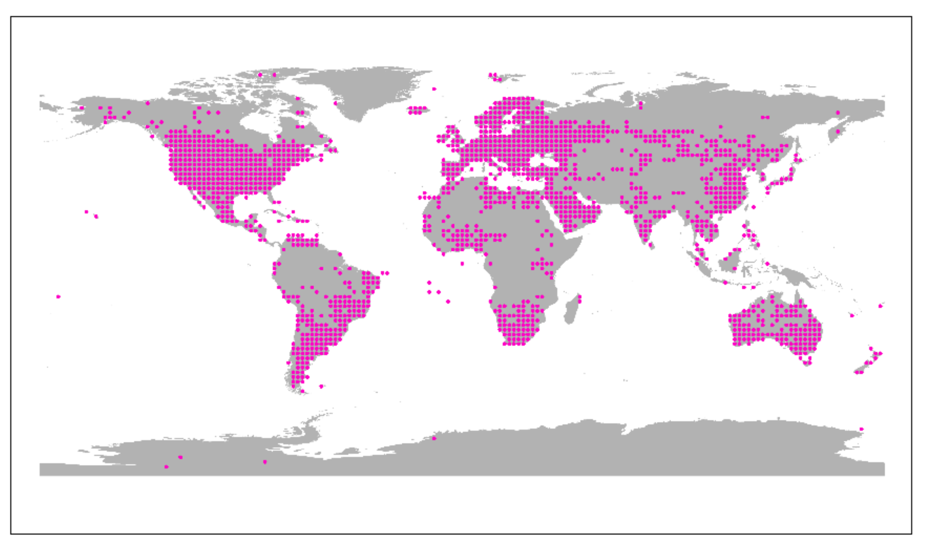
2.3. Validation Data Preparation
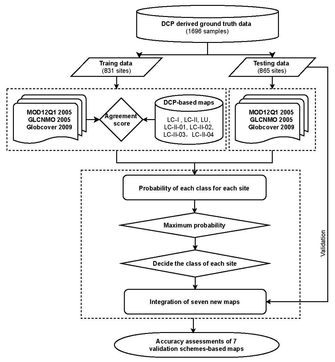
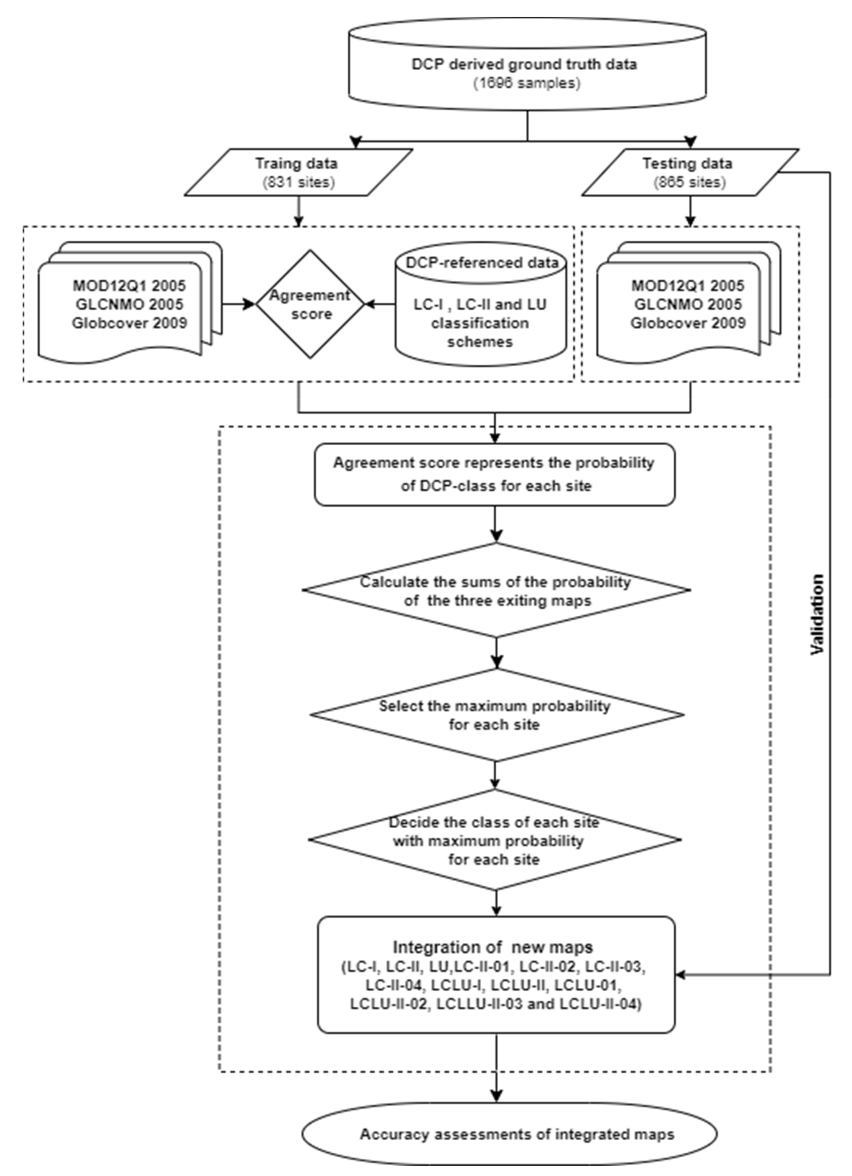
2.4. Comparison between DCP-Based Ground Truth Data and Existing Maps
2.5. Integration of New Maps
3. Results
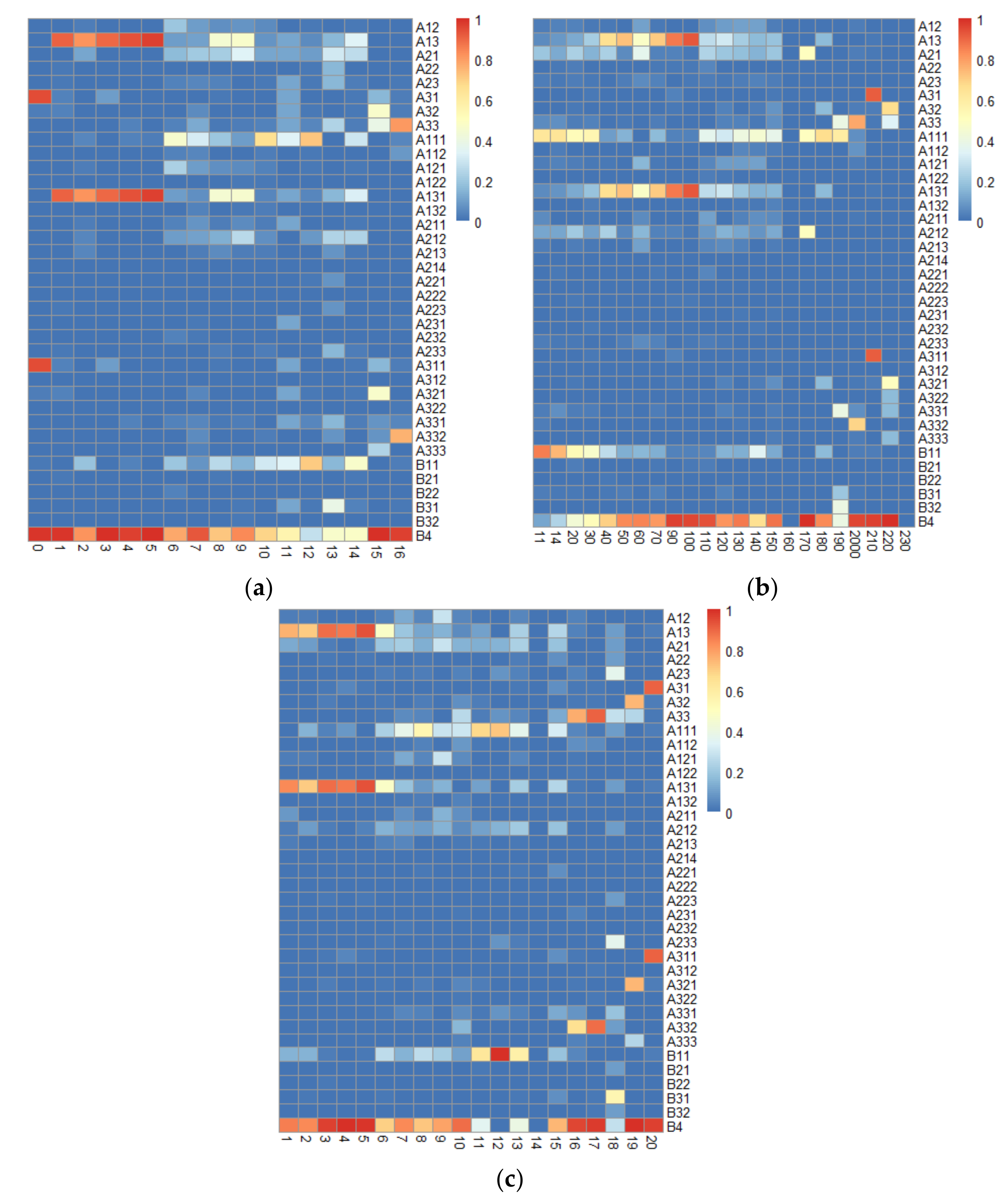
3.1. Agreement Analysis between DCP Data and Three Global Land-Cover Products
3.1.1. Grassland Classes
3.1.2. Mosaic Classes
3.1.3. Urban and Built-Up Classes
3.1.4. Bare Area Classes
3.1.5. Water-Related Classes
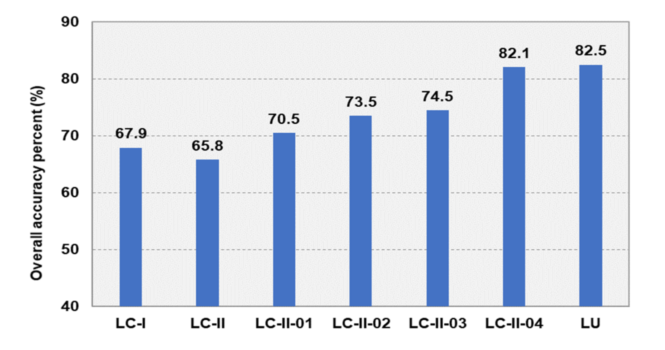
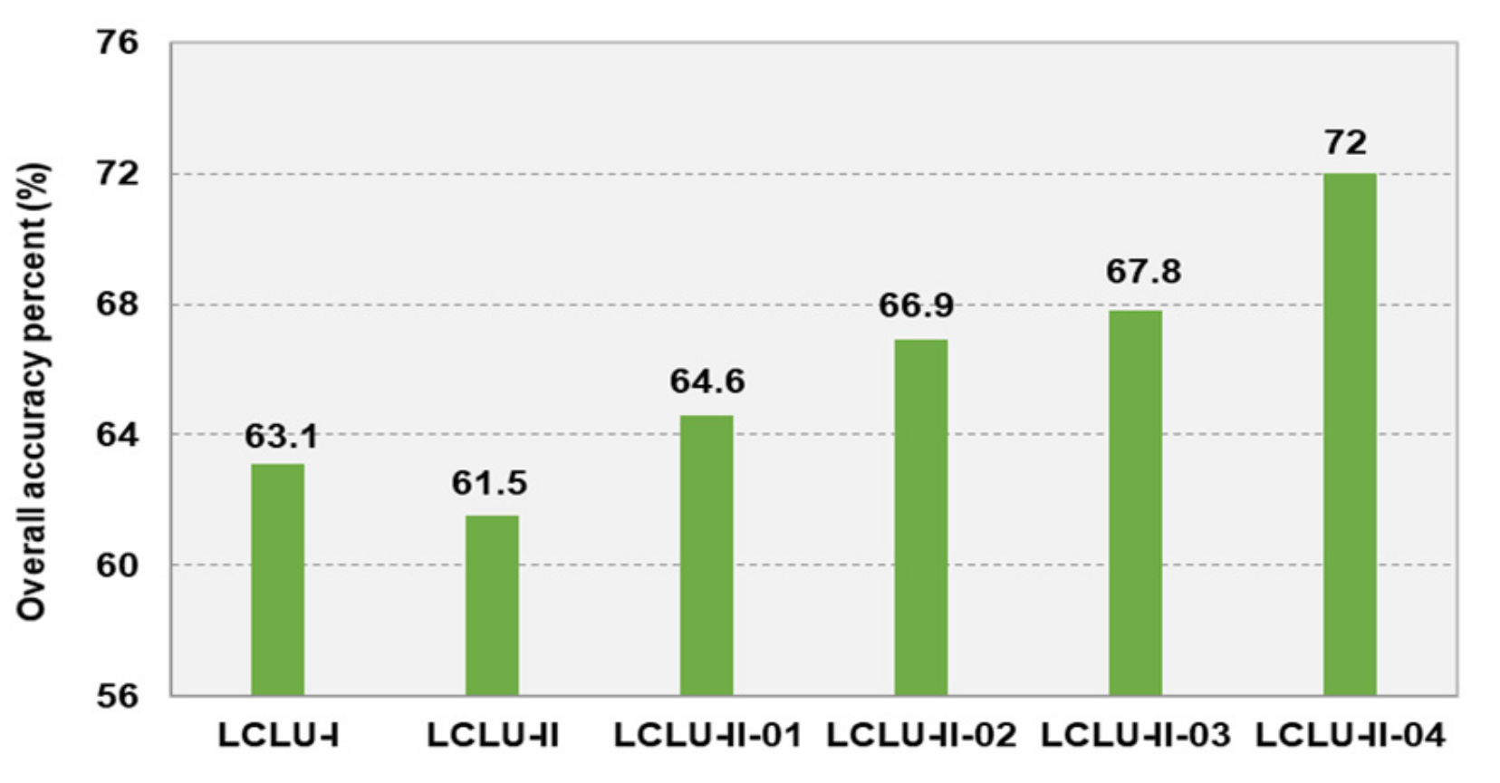
3.2. Assessing the Accuracy of Classification Datasets
4. Discussion
4.1. Analysis of Validation Data Uncertainty
4.2. Analysis of Classification Schemes
4.3. Suggestions and Future Research Directions
5. Conclusions
Author Contributions
Funding
Acknowledgments
Conflicts of Interest
Appendix A

| 0 | 1 | 2 | 3 | 4 | 5 | 6 | 7 | 8 | 9 | 10 | 11 | 12 | 13 | 14 | 15 | 16 | SUM | |
| A11 | 1 | 0 | 2 | 0 | 1 | 3 | 15 | 71 | 23 | 8 | 141 | 3 | 219 | 0 | 50 | 0 | 18 | 555 |
| A12 | 0 | 0 | 1 | 0 | 0 | 0 | 6 | 19 | 8 | 6 | 11 | 0 | 4 | 0 | 2 | 0 | 1 | 58 |
| A13 | 0 | 78 | 36 | 9 | 27 | 119 | 3 | 20 | 52 | 39 | 16 | 1 | 16 | 2 | 56 | 0 | 0 | 474 |
| A21 | 1 | 0 | 5 | 0 | 0 | 1 | 5 | 40 | 25 | 28 | 24 | 1 | 27 | 4 | 45 | 0 | 1 | 207 |
| A22 | 1 | 1 | 0 | 0 | 0 | 0 | 0 | 2 | 1 | 0 | 1 | 0 | 6 | 2 | 1 | 0 | 0 | 15 |
| A23 | 0 | 1 | 0 | 0 | 0 | 0 | 1 | 8 | 4 | 0 | 3 | 1 | 4 | 2 | 5 | 0 | 2 | 31 |
| A31 | 122 | 3 | 0 | 1 | 0 | 0 | 0 | 1 | 2 | 0 | 1 | 1 | 1 | 0 | 2 | 2 | 3 | 139 |
| A32 | 3 | 3 | 0 | 0 | 0 | 0 | 0 | 10 | 1 | 0 | 2 | 1 | 6 | 0 | 2 | 6 | 3 | 37 |
| A33 | 1 | 0 | 0 | 0 | 1 | 0 | 1 | 25 | 2 | 2 | 8 | 1 | 15 | 3 | 5 | 5 | 116 | 185 |
| SUM | 129 | 86 | 44 | 10 | 29 | 123 | 31 | 196 | 118 | 83 | 207 | 9 | 298 | 13 | 168 | 13 | 144 | 1701 |
| 0 | 1 | 2 | 3 | 4 | 5 | 6 | 7 | 8 | 9 | 10 | 11 | 12 | 13 | 14 | 15 | 16 | SUM | |
| A111 | 1 | 0 | 2 | 0 | 1 | 3 | 14 | 62 | 23 | 8 | 136 | 3 | 214 | 0 | 50 | 0 | 6 | 523 |
| A112 | 0 | 0 | 0 | 0 | 0 | 0 | 1 | 9 | 0 | 0 | 5 | 0 | 5 | 0 | 0 | 0 | 12 | 32 |
| A121 | 0 | 0 | 1 | 0 | 0 | 0 | 7 | 19 | 8 | 5 | 8 | 0 | 4 | 0 | 2 | 0 | 1 | 55 |
| A122 | 0 | 0 | 0 | 0 | 0 | 0 | 0 | 1 | 0 | 1 | 3 | 0 | 0 | 0 | 0 | 0 | 0 | 5 |
| A131 | 0 | 78 | 36 | 9 | 27 | 119 | 3 | 13 | 52 | 38 | 10 | 1 | 15 | 2 | 55 | 0 | 0 | 458 |
| A132 | 0 | 0 | 0 | 0 | 0 | 0 | 0 | 6 | 0 | 1 | 5 | 0 | 1 | 0 | 1 | 0 | 0 | 14 |
| A211 | 0 | 0 | 1 | 0 | 0 | 0 | 1 | 15 | 3 | 5 | 5 | 1 | 2 | 0 | 2 | 0 | 0 | 35 |
| A212 | 1 | 0 | 2 | 0 | 0 | 1 | 3 | 20 | 16 | 21 | 13 | 0 | 25 | 3 | 40 | 0 | 1 | 146 |
| A213 | 0 | 0 | 2 | 0 | 0 | 0 | 0 | 5 | 6 | 2 | 5 | 0 | 0 | 1 | 3 | 0 | 0 | 24 |
| A214 | 0 | 0 | 0 | 0 | 0 | 0 | 0 | 0 | 0 | 0 | 0 | 0 | 0 | 0 | 0 | 0 | 0 | 0 |
| A221 | 0 | 0 | 0 | 0 | 0 | 0 | 0 | 2 | 1 | 0 | 1 | 0 | 5 | 1 | 0 | 0 | 0 | 10 |
| A222 | 0 | 0 | 0 | 0 | 0 | 0 | 0 | 0 | 0 | 0 | 0 | 0 | 0 | 0 | 0 | 0 | 0 | 0 |
| A223 | 1 | 1 | 0 | 0 | 0 | 0 | 0 | 0 | 0 | 0 | 0 | 0 | 1 | 1 | 1 | 0 | 0 | 5 |
| A231 | 0 | 0 | 0 | 0 | 0 | 0 | 0 | 3 | 1 | 0 | 0 | 1 | 1 | 0 | 0 | 0 | 2 | 8 |
| A232 | 0 | 0 | 0 | 0 | 0 | 0 | 1 | 3 | 0 | 0 | 0 | 0 | 2 | 0 | 0 | 0 | 0 | 6 |
| A233 | 0 | 1 | 0 | 0 | 0 | 0 | 0 | 2 | 3 | 0 | 5 | 0 | 1 | 2 | 5 | 0 | 0 | 19 |
| A311 | 122 | 3 | 0 | 1 | 0 | 0 | 0 | 0 | 2 | 0 | 1 | 1 | 1 | 0 | 2 | 2 | 3 | 138 |
| A312 | 0 | 0 | 0 | 0 | 0 | 0 | 0 | 1 | 0 | 0 | 0 | 0 | 0 | 0 | 0 | 0 | 0 | 1 |
| A321 | 3 | 3 | 0 | 0 | 0 | 0 | 0 | 9 | 1 | 0 | 2 | 1 | 6 | 0 | 2 | 6 | 1 | 34 |
| A322 | 0 | 0 | 0 | 0 | 0 | 0 | 0 | 1 | 0 | 0 | 0 | 0 | 0 | 0 | 0 | 0 | 2 | 3 |
| A331 | 0 | 0 | 0 | 0 | 1 | 0 | 1 | 9 | 2 | 2 | 2 | 1 | 13 | 2 | 5 | 1 | 6 | 45 |
| A332 | 1 | 0 | 0 | 0 | 0 | 0 | 0 | 10 | 0 | 0 | 5 | 0 | 2 | 1 | 0 | 1 | 109 | 129 |
| A333 | 0 | 0 | 0 | 0 | 0 | 0 | 0 | 6 | 0 | 0 | 1 | 0 | 0 | 0 | 0 | 3 | 1 | 11 |
| SUM | 129 | 86 | 44 | 10 | 29 | 123 | 31 | 196 | 118 | 83 | 207 | 9 | 298 | 13 | 168 | 13 | 144 | 1701 |
| 0 | 1 | 2 | 3 | 4 | 5 | 6 | 7 | 8 | 9 | 10 | 11 | 12 | 13 | 14 | 15 | 16 | SUM | |
| B11 | 2 | 0 | 8 | 0 | 1 | 1 | 6 | 14 | 30 | 12 | 63 | 3 | 209 | 2 | 79 | 0 | 3 | 433 |
| B21 | 0 | 1 | 0 | 0 | 0 | 0 | 0 | 0 | 2 | 0 | 0 | 0 | 2 | 0 | 3 | 0 | 0 | 8 |
| B22 | 0 | 0 | 0 | 0 | 0 | 0 | 1 | 0 | 0 | 0 | 0 | 0 | 1 | 0 | 0 | 0 | 0 | 2 |
| B31 | 0 | 0 | 0 | 0 | 0 | 0 | 0 | 0 | 1 | 1 | 1 | 1 | 4 | 5 | 6 | 0 | 2 | 21 |
| B32 | 0 | 0 | 0 | 0 | 0 | 0 | 0 | 1 | 0 | 1 | 1 | 0 | 1 | 0 | 0 | 0 | 0 | 4 |
| B4 | 127 | 85 | 36 | 10 | 28 | 122 | 24 | 181 | 85 | 69 | 142 | 5 | 81 | 6 | 80 | 13 | 139 | 1233 |
| SUM | 129 | 86 | 44 | 10 | 29 | 123 | 31 | 196 | 118 | 83 | 207 | 9 | 298 | 13 | 168 | 13 | 144 | 1701 |
| 11 | 14 | 20 | 30 | 40 | 50 | 60 | 70 | 90 | 100 | 110 | 120 | 130 | 140 | 150 | 160 | 170 | 180 | 190 | 200 | 210 | 220 | 230 | SUM | |
| A11 | 22 | 108 | 73 | 83 | 5 | 20 | 0 | 13 | 2 | 2 | 17 | 17 | 55 | 52 | 53 | 0 | 1 | 4 | 3 | 25 | 1 | 0 | 0 | 556 |
| A12 | 1 | 5 | 5 | 3 | 1 | 1 | 2 | 1 | 0 | 0 | 3 | 5 | 13 | 11 | 3 | 0 | 0 | 0 | 0 | 4 | 0 | 0 | 0 | 58 |
| A13 | 2 | 14 | 18 | 32 | 35 | 97 | 9 | 56 | 51 | 58 | 12 | 17 | 26 | 18 | 25 | 0 | 0 | 1 | 0 | 1 | 2 | 0 | 0 | 474 |
| A21 | 7 | 20 | 32 | 22 | 12 | 8 | 7 | 3 | 2 | 1 | 11 | 11 | 22 | 16 | 26 | 0 | 1 | 0 | 0 | 4 | 2 | 0 | 0 | 207 |
| A22 | 0 | 2 | 3 | 1 | 0 | 1 | 0 | 1 | 1 | 1 | 2 | 0 | 0 | 1 | 1 | 0 | 0 | 0 | 0 | 0 | 1 | 0 | 0 | 15 |
| A23 | 1 | 3 | 3 | 2 | 0 | 3 | 1 | 3 | 0 | 1 | 1 | 1 | 3 | 4 | 3 | 0 | 0 | 0 | 0 | 1 | 0 | 0 | 0 | 30 |
| A31 | 0 | 0 | 0 | 2 | 0 | 0 | 0 | 0 | 2 | 0 | 0 | 0 | 0 | 1 | 2 | 0 | 0 | 0 | 0 | 1 | 131 | 0 | 0 | 139 |
| A32 | 0 | 1 | 2 | 0 | 0 | 1 | 0 | 0 | 1 | 0 | 0 | 2 | 0 | 3 | 10 | 0 | 0 | 1 | 0 | 4 | 4 | 4 | 0 | 33 |
| A33 | 2 | 10 | 3 | 5 | 0 | 2 | 0 | 2 | 0 | 0 | 0 | 2 | 4 | 2 | 9 | 0 | 0 | 0 | 2 | 137 | 2 | 2 | 0 | 184 |
| SUM | 35 | 163 | 139 | 150 | 53 | 133 | 19 | 79 | 59 | 63 | 46 | 55 | 123 | 108 | 132 | 0 | 2 | 6 | 5 | 177 | 143 | 6 | 0 | 1696 |
| 11 | 14 | 20 | 30 | 40 | 50 | 60 | 70 | 90 | 100 | 110 | 120 | 130 | 140 | 150 | 160 | 170 | 180 | 190 | 200 | 210 | 220 | 230 | SUM | |
| A111 | 22 | 104 | 72 | 82 | 5 | 20 | 0 | 13 | 2 | 2 | 17 | 17 | 50 | 48 | 49 | 0 | 1 | 4 | 3 | 12 | 1 | 0 | 0 | 524 |
| A112 | 0 | 4 | 1 | 1 | 0 | 0 | 0 | 0 | 0 | 0 | 0 | 0 | 5 | 4 | 4 | 0 | 0 | 0 | 0 | 13 | 0 | 0 | 0 | 32 |
| A121 | 1 | 5 | 4 | 3 | 1 | 1 | 3 | 1 | 0 | 0 | 2 | 5 | 12 | 11 | 2 | 0 | 0 | 0 | 0 | 4 | 0 | 0 | 0 | 55 |
| A122 | 0 | 0 | 1 | 0 | 0 | 0 | 0 | 0 | 0 | 0 | 1 | 1 | 1 | 0 | 1 | 0 | 0 | 0 | 0 | 0 | 0 | 0 | 0 | 5 |
| A131 | 2 | 13 | 18 | 28 | 35 | 97 | 9 | 56 | 51 | 58 | 12 | 16 | 24 | 16 | 20 | 0 | 0 | 1 | 0 | 0 | 2 | 0 | 0 | 458 |
| A132 | 0 | 1 | 0 | 4 | 0 | 0 | 0 | 0 | 0 | 0 | 0 | 0 | 2 | 2 | 5 | 0 | 0 | 0 | 0 | 1 | 0 | 0 | 0 | 15 |
| A211 | 2 | 0 | 1 | 3 | 0 | 1 | 1 | 0 | 0 | 0 | 5 | 0 | 4 | 7 | 7 | 0 | 0 | 0 | 0 | 3 | 1 | 0 | 0 | 35 |
| A212 | 4 | 19 | 28 | 16 | 12 | 6 | 3 | 3 | 2 | 1 | 4 | 8 | 14 | 8 | 16 | 0 | 1 | 0 | 0 | 1 | 1 | 0 | 0 | 147 |
| A213 | 1 | 1 | 3 | 3 | 0 | 1 | 2 | 0 | 0 | 0 | 2 | 3 | 4 | 1 | 3 | 0 | 0 | 0 | 0 | 0 | 0 | 0 | 0 | 24 |
| A214 | 0 | 0 | 0 | 0 | 0 | 0 | 0 | 0 | 0 | 0 | 0 | 0 | 0 | 0 | 0 | 0 | 0 | 0 | 0 | 0 | 0 | 0 | 0 | 0 |
| A221 | 0 | 2 | 1 | 1 | 0 | 1 | 0 | 1 | 0 | 0 | 2 | 0 | 0 | 1 | 1 | 0 | 0 | 0 | 0 | 0 | 0 | 0 | 0 | 10 |
| A222 | 0 | 0 | 0 | 0 | 0 | 0 | 0 | 0 | 0 | 0 | 0 | 0 | 0 | 0 | 0 | 0 | 0 | 0 | 0 | 0 | 0 | 0 | 0 | 0 |
| A223 | 0 | 0 | 2 | 0 | 0 | 0 | 0 | 0 | 1 | 1 | 0 | 0 | 0 | 0 | 0 | 0 | 0 | 0 | 0 | 0 | 1 | 0 | 0 | 5 |
| A231 | 0 | 0 | 1 | 0 | 0 | 0 | 0 | 0 | 0 | 0 | 0 | 0 | 2 | 1 | 2 | 0 | 0 | 0 | 0 | 1 | 0 | 0 | 0 | 7 |
| A232 | 0 | 1 | 0 | 2 | 0 | 0 | 0 | 0 | 0 | 0 | 0 | 0 | 0 | 2 | 1 | 0 | 0 | 0 | 0 | 0 | 0 | 0 | 0 | 6 |
| A233 | 1 | 2 | 2 | 0 | 0 | 3 | 1 | 3 | 0 | 1 | 1 | 1 | 1 | 1 | 0 | 0 | 0 | 0 | 0 | 0 | 0 | 0 | 0 | 17 |
| A311 | 0 | 0 | 0 | 2 | 0 | 0 | 0 | 0 | 2 | 0 | 0 | 0 | 0 | 1 | 2 | 0 | 0 | 0 | 0 | 0 | 131 | 0 | 0 | 138 |
| A312 | 0 | 0 | 0 | 0 | 0 | 0 | 0 | 0 | 0 | 0 | 0 | 0 | 0 | 0 | 0 | 0 | 0 | 0 | 0 | 1 | 0 | 0 | 0 | 1 |
| A321 | 0 | 1 | 2 | 0 | 0 | 1 | 0 | 0 | 1 | 0 | 0 | 2 | 0 | 3 | 9 | 0 | 0 | 1 | 0 | 3 | 4 | 3 | 0 | 30 |
| A322 | 0 | 0 | 0 | 0 | 0 | 0 | 0 | 0 | 0 | 0 | 0 | 0 | 0 | 0 | 1 | 0 | 0 | 0 | 0 | 1 | 0 | 1 | 0 | 3 |
| A331 | 1 | 10 | 3 | 4 | 0 | 2 | 0 | 2 | 0 | 0 | 0 | 2 | 2 | 1 | 3 | 0 | 0 | 0 | 2 | 11 | 1 | 1 | 0 | 45 |
| A332 | 1 | 0 | 0 | 1 | 0 | 0 | 0 | 0 | 0 | 0 | 0 | 0 | 2 | 1 | 2 | 0 | 0 | 0 | 0 | 121 | 1 | 0 | 0 | 129 |
| A333 | 0 | 0 | 0 | 0 | 0 | 0 | 0 | 0 | 0 | 0 | 0 | 0 | 0 | 0 | 4 | 0 | 0 | 0 | 0 | 5 | 0 | 1 | 0 | 10 |
| SUM | 35 | 163 | 139 | 150 | 53 | 133 | 19 | 79 | 59 | 63 | 46 | 55 | 123 | 108 | 132 | 0 | 2 | 6 | 5 | 177 | 143 | 6 | 0 | 1696 |
| 11 | 14 | 20 | 30 | 40 | 50 | 60 | 70 | 90 | 100 | 110 | 120 | 130 | 140 | 150 | 160 | 170 | 180 | 190 | 200 | 210 | 220 | 230 | SUM | |
| B11 | 30 | 121 | 73 | 70 | 14 | 18 | 3 | 11 | 2 | 2 | 2 | 8 | 17 | 37 | 16 | 0 | 0 | 1 | 0 | 4 | 4 | 0 | 0 | 433 |
| B21 | 0 | 1 | 3 | 0 | 0 | 1 | 0 | 1 | 0 | 1 | 1 | 0 | 0 | 0 | 0 | 0 | 0 | 0 | 0 | 0 | 0 | 0 | 0 | 8 |
| B22 | 0 | 0 | 0 | 1 | 1 | 0 | 0 | 0 | 0 | 0 | 0 | 0 | 0 | 0 | 0 | 0 | 0 | 0 | 0 | 0 | 0 | 0 | 0 | 2 |
| B31 | 1 | 3 | 2 | 1 | 1 | 3 | 0 | 3 | 0 | 0 | 0 | 2 | 0 | 0 | 0 | 0 | 0 | 0 | 1 | 3 | 1 | 0 | 0 | 21 |
| B32 | 0 | 0 | 0 | 1 | 0 | 0 | 0 | 0 | 0 | 0 | 0 | 0 | 0 | 0 | 0 | 0 | 0 | 0 | 2 | 1 | 0 | 0 | 0 | 4 |
| B4 | 4 | 38 | 61 | 77 | 37 | 111 | 16 | 64 | 57 | 60 | 43 | 45 | 106 | 71 | 116 | 0 | 2 | 5 | 2 | 169 | 138 | 6 | 0 | 1228 |
| SUM | 35 | 163 | 139 | 150 | 53 | 133 | 19 | 79 | 59 | 63 | 46 | 55 | 123 | 108 | 132 | 0 | 2 | 6 | 5 | 177 | 143 | 6 | 0 | 1696 |
| 1 | 2 | 3 | 4 | 5 | 6 | 7 | 8 | 9 | 10 | 11 | 12 | 13 | 14 | 15 | 16 | 17 | 18 | 19 | 20 | SUM | |
| A11 | 4 | 14 | 3 | 2 | 0 | 44 | 60 | 119 | 4 | 39 | 193 | 10 | 43 | 0 | 5 | 7 | 5 | 1 | 0 | 3 | 556 |
| A12 | 1 | 3 | 0 | 0 | 0 | 6 | 19 | 10 | 4 | 5 | 3 | 0 | 5 | 0 | 0 | 2 | 0 | 0 | 0 | 0 | 58 |
| A13 | 31 | 70 | 73 | 20 | 59 | 93 | 30 | 24 | 2 | 6 | 31 | 0 | 25 | 0 | 4 | 2 | 0 | 1 | 0 | 3 | 474 |
| A21 | 5 | 9 | 2 | 0 | 2 | 39 | 34 | 27 | 4 | 15 | 37 | 2 | 26 | 0 | 3 | 0 | 0 | 1 | 0 | 1 | 207 |
| A22 | 0 | 1 | 1 | 0 | 1 | 1 | 0 | 4 | 0 | 0 | 2 | 0 | 3 | 0 | 1 | 0 | 0 | 1 | 0 | 0 | 15 |
| A23 | 0 | 1 | 0 | 0 | 0 | 5 | 2 | 5 | 0 | 4 | 2 | 1 | 4 | 0 | 0 | 2 | 0 | 4 | 0 | 0 | 30 |
| A31 | 0 | 0 | 1 | 1 | 1 | 1 | 0 | 1 | 0 | 1 | 0 | 0 | 2 | 0 | 1 | 1 | 1 | 0 | 0 | 128 | 139 |
| A32 | 0 | 0 | 2 | 0 | 0 | 3 | 1 | 6 | 0 | 7 | 6 | 0 | 0 | 0 | 0 | 1 | 1 | 0 | 6 | 4 | 37 |
| A33 | 0 | 1 | 0 | 0 | 0 | 4 | 9 | 9 | 0 | 26 | 7 | 1 | 5 | 0 | 2 | 48 | 66 | 3 | 2 | 2 | 185 |
| SUM | 41 | 99 | 82 | 23 | 63 | 196 | 155 | 205 | 14 | 103 | 281 | 14 | 113 | 0 | 16 | 63 | 73 | 11 | 8 | 141 | 1701 |
| 1 | 2 | 3 | 4 | 5 | 6 | 7 | 8 | 9 | 10 | 11 | 12 | 13 | 14 | 15 | 16 | 17 | 18 | 19 | 20 | SUM | |
| A111 | 0 | 14 | 3 | 2 | 0 | 44 | 58 | 112 | 4 | 30 | 189 | 10 | 41 | 0 | 5 | 3 | 1 | 1 | 0 | 3 | 520 |
| A112 | 0 | 0 | 0 | 0 | 0 | 0 | 2 | 7 | 0 | 9 | 4 | 0 | 2 | 0 | 0 | 4 | 4 | 0 | 0 | 0 | 32 |
| A121 | 1 | 3 | 0 | 0 | 0 | 5 | 20 | 9 | 4 | 6 | 1 | 0 | 5 | 0 | 0 | 1 | 0 | 0 | 0 | 0 | 55 |
| A122 | 0 | 0 | 0 | 0 | 0 | 1 | 0 | 1 | 0 | 0 | 2 | 0 | 0 | 0 | 0 | 1 | 0 | 0 | 0 | 0 | 5 |
| A131 | 31 | 70 | 73 | 20 | 59 | 93 | 28 | 18 | 2 | 1 | 30 | 0 | 24 | 0 | 4 | 1 | 0 | 1 | 0 | 3 | 458 |
| A132 | 0 | 0 | 0 | 0 | 0 | 0 | 2 | 6 | 0 | 4 | 1 | 0 | 1 | 0 | 0 | 1 | 0 | 0 | 0 | 0 | 15 |
| A211 | 3 | 0 | 0 | 0 | 0 | 4 | 10 | 5 | 2 | 7 | 3 | 0 | 1 | 0 | 0 | 0 | 0 | 0 | 0 | 0 | 35 |
| A212 | 1 | 9 | 2 | 0 | 2 | 28 | 16 | 20 | 2 | 6 | 31 | 2 | 23 | 0 | 3 | 0 | 0 | 1 | 0 | 1 | 147 |
| A213 | 1 | 0 | 0 | 0 | 0 | 7 | 7 | 2 | 0 | 2 | 3 | 0 | 2 | 0 | 0 | 0 | 0 | 0 | 0 | 0 | 24 |
| A214 | 0 | 0 | 0 | 0 | 0 | 0 | 0 | 0 | 0 | 0 | 0 | 0 | 0 | 0 | 0 | 0 | 0 | 0 | 0 | 0 | 0 |
| A221 | 0 | 1 | 0 | 0 | 0 | 1 | 0 | 4 | 0 | 0 | 1 | 0 | 2 | 0 | 1 | 0 | 0 | 0 | 0 | 0 | 10 |
| A222 | 0 | 0 | 0 | 0 | 0 | 0 | 0 | 0 | 0 | 0 | 0 | 0 | 0 | 0 | 0 | 0 | 0 | 0 | 0 | 0 | 0 |
| A223 | 0 | 0 | 1 | 0 | 1 | 0 | 0 | 0 | 0 | 0 | 1 | 0 | 1 | 0 | 0 | 0 | 0 | 1 | 0 | 0 | 5 |
| A231 | 0 | 0 | 0 | 0 | 0 | 1 | 0 | 1 | 0 | 2 | 0 | 0 | 1 | 0 | 0 | 2 | 0 | 0 | 0 | 0 | 7 |
| A232 | 0 | 0 | 0 | 0 | 0 | 1 | 2 | 2 | 0 | 1 | 0 | 0 | 0 | 0 | 0 | 0 | 0 | 0 | 0 | 0 | 6 |
| A233 | 0 | 1 | 0 | 0 | 0 | 3 | 0 | 2 | 0 | 1 | 2 | 1 | 3 | 0 | 0 | 0 | 0 | 4 | 0 | 0 | 17 |
| A311 | 0 | 0 | 1 | 1 | 1 | 1 | 0 | 1 | 0 | 1 | 0 | 0 | 2 | 0 | 1 | 1 | 0 | 0 | 0 | 128 | 138 |
| A312 | 0 | 0 | 0 | 0 | 0 | 0 | 0 | 0 | 0 | 0 | 0 | 0 | 0 | 0 | 0 | 0 | 1 | 0 | 0 | 0 | 1 |
| A321 | 0 | 0 | 2 | 0 | 0 | 3 | 1 | 6 | 0 | 5 | 6 | 0 | 0 | 0 | 0 | 1 | 0 | 0 | 6 | 4 | 34 |
| A322 | 0 | 0 | 0 | 0 | 0 | 0 | 0 | 0 | 0 | 2 | 0 | 0 | 0 | 0 | 0 | 0 | 1 | 0 | 0 | 0 | 3 |
| A331 | 0 | 1 | 0 | 0 | 0 | 4 | 7 | 7 | 0 | 6 | 5 | 1 | 4 | 0 | 2 | 5 | 0 | 2 | 0 | 1 | 45 |
| A332 | 0 | 0 | 0 | 0 | 0 | 0 | 1 | 1 | 0 | 16 | 2 | 0 | 1 | 0 | 0 | 41 | 65 | 1 | 0 | 1 | 129 |
| A333 | 0 | 0 | 0 | 0 | 0 | 0 | 1 | 1 | 0 | 4 | 0 | 0 | 0 | 0 | 0 | 2 | 1 | 0 | 2 | 0 | 11 |
| SUM | 37 | 99 | 82 | 23 | 63 | 196 | 155 | 205 | 14 | 103 | 281 | 14 | 113 | 0 | 16 | 63 | 73 | 11 | 8 | 141 | 1697 |
| 1 | 2 | 3 | 4 | 5 | 6 | 7 | 8 | 9 | 10 | 11 | 12 | 13 | 14 | 15 | 16 | 17 | 18 | 19 | 20 | SUM | |
| B11 | 6 | 14 | 2 | 0 | 1 | 53 | 23 | 54 | 3 | 11 | 177 | 14 | 65 | 0 | 3 | 3 | 0 | 0 | 0 | 4 | 433 |
| B21 | 0 | 0 | 0 | 0 | 0 | 2 | 0 | 1 | 0 | 0 | 3 | 0 | 1 | 0 | 0 | 0 | 0 | 1 | 0 | 0 | 8 |
| B22 | 0 | 0 | 1 | 0 | 0 | 0 | 0 | 1 | 0 | 0 | 0 | 0 | 0 | 0 | 0 | 0 | 0 | 0 | 0 | 0 | 2 |
| B31 | 0 | 2 | 0 | 0 | 0 | 4 | 1 | 1 | 0 | 1 | 1 | 0 | 2 | 0 | 1 | 0 | 1 | 6 | 0 | 1 | 21 |
| B32 | 0 | 0 | 0 | 0 | 0 | 0 | 1 | 1 | 0 | 0 | 0 | 0 | 0 | 0 | 0 | 0 | 1 | 1 | 0 | 0 | 4 |
| B4 | 35 | 83 | 79 | 23 | 62 | 137 | 130 | 147 | 11 | 91 | 100 | 0 | 45 | 0 | 12 | 60 | 71 | 3 | 8 | 136 | 1233 |
| SUM | 41 | 99 | 82 | 23 | 63 | 196 | 155 | 205 | 14 | 103 | 281 | 14 | 113 | 0 | 16 | 63 | 73 | 11 | 8 | 141 | 1701 |
References
- Barnett, J. Security and climate change. Global Environ. Chang. 2003, 13, 7–17. [Google Scholar] [CrossRef]
- Huadong, G.; Stefano, N.; Dong, L.; Max, C.; Lizhe, W.; Sven, S.; Christina, C.; Guojin, H.; Martino, P.; Jianhui, L.; et al. Big Earth Data science: an information framework for a sustainable planet. Int. J. Digit. Earth 2020, 13, 743–767. [Google Scholar]
- Onoda, M.; Young, O.R. Satellite Earth Observations and Their Impact on Society and Policy; Springer Open: Singapore, 2017. [Google Scholar]
- Mora, B.; Tsendbazar, N.E.; Herold, M.; Arino, O. Global Land Cover Mapping: Current Status and Future Trends; Springer: Dordrecht, The Netherlands, 2014. [Google Scholar]
- Michael, A.W.; Nicholas, C.C.; David, P.R.; Joanne, C.W.T.H. Land cover 2.0. Int. J. Remote Sens. 2018, 39, 4254–4284. [Google Scholar]
- Stehman, S.V.; Fonte, C.C.; Foody, G.M.; See, L. Using volunteered geographic information (VGI) in design-based statistical inference for area estimation and accuracy assessment of land cover. Remote Sens. Environ. 2018, 212, 47–59. [Google Scholar] [CrossRef]
- Strahler, A.H.; Boschetti, L.; Foody, G.M.; Friedl, M.A.; Hansen, M.C.; Herold, M.; Mayaux, P.; Morisette, J.T.; Stehman, S.V.; Woodcock, C.E. Global Land Cover Validation: Recommendations for Evaluation and Accuracy Assessment of Global Land Cover Maps. In Technical Report EUR 22156 EN-DG 2006; Office for Official Publications of the European Community: Luxembourg, 2006. [Google Scholar]
- Olofsson, P.; Foody, G.M.; Herold, M.; Stehman, S.V.; Woodcock, C.E.; Wulder, M.A. Good practices for estimating area and assessing accuracy of land change. Remote Sens. Environ. 2014, 148, 42–57. [Google Scholar] [CrossRef]
- McRoberts, R.E.; Stehman, S.V.; Liknes, G.C.; Næsset, E.; Sannier, C.; Walters, B.F. The effects of imperfect reference data on remote sensing-assisted estimators of land cover class proportions. ISPRS J. Photogramm. Remote Sens. 2018, 142, 292–300. [Google Scholar] [CrossRef]
- Muchoney, D.M.; Borak, J.; Strahler, A. Global landcover classification validation issues and requirements. In Proceedings of the International Geoscience and Remote Sensing Symposium, Lincoln, NE, USA, 27–31 May 1996; pp. 233–235. [Google Scholar]
- Stehman, S.V.; Czaplewski, R.L. Design and analysis for thematic map accuracy assessment: Fundamental principles. Remote Sens. Environ. 1998, 64, 331–344. [Google Scholar] [CrossRef]
- Klein, G.K.; Ramankutty, N. Land cover change over the last three centuries due to human activities: The availability of new global data sets. GeoJournal 2004, 61, 335–344. [Google Scholar] [CrossRef]
- Morisette, J.T.; Nickeson, J.E.; Davis, P.; Wang, Y.; Tian, Y.; Woodcock, C.E.; Shabanov, N.; Hansen, M.; Cohen, W.B.; Oetter, D.R.; et al. High spatial resolution satellite observations for validation of MODIS land products: IKONOS observations acquired under the NASA Scientific Data Purchase. Remote Sens. Environ. 2003, 88, 100–110. [Google Scholar] [CrossRef]
- Wulder, M.A.; Boots, B.; Seemann, D.; White, J.C. Map comparison using spatial autocorrelation: An example using AVHRR derived land cover of Canada. Can. J. Remote Sens. 2004, 30, 573–592. [Google Scholar] [CrossRef]
- Pengra, B.; Long, J.; Dahal, D.; Stehman, S.V.; Loveland, T.R. A global reference database from very high resolution commercial satellite data and methodology for application to Landsat derived 30 m continuous field tree cover data. Remote Sens. Environ. 2015, 165, 234–248. [Google Scholar] [CrossRef]
- Midekisa, A.; Holl, F.; Savory, D.J.; Andrade-Pacheco, R.; Gething, P.W.; Bennett, A.; Sturrock, H.J.W. Mapping land cover change over continental Africa using Landsat and Google Earth Engine cloud computing. PLoS ONE 2017, 12, 1–15. [Google Scholar] [CrossRef] [PubMed]
- Sun, B.; Chen, X.; Zhou, Q. Uncertainty assessment of GlobeLand30 Land cover data set over central Asia. ISPRS - Int. Arch. Photogramm. Remote Sens. Spat. Inf. Sci. 2016, 41, 1313–1317. [Google Scholar] [CrossRef]
- Ozdogan, M.; Woodcock, C.E. Resolution dependent errors in remote sensing of cultivated areas. Remote Sens. Environ. 2006, 103, 203–217. [Google Scholar] [CrossRef]
- Foody, G.M. Ground reference data error and the mis-estimation of the area of land cover change as a function of its abundance. Remote Sens. Lett. 2013, 4, 783–792. [Google Scholar] [CrossRef]
- Zhao, Y.; Gong, P.; Yu, L.; Hu, L.; Li, X.; Li, C.; Zhang, H.; Zheng, Y.; Wang, J.; Zhao, Y.; et al. Towards a common validation sample set for global land-cover mapping. Int. J. Remote Sens. 2014, 35, 4795–4814. [Google Scholar] [CrossRef]
- O’Reilly, T. What is Web 2.0: Design Patterns and Business Models for the Next Generation of Software. 2005. Available online: https://www.oreilly.com/pub/a/web2/archive/what-is-web-20.html (accessed on 1 May 2020).
- Goodchild, M.F.; Fu, P.; Rich, P. Sharing geographic information: An assessment of the geospatial one-stop. Ann. Assoc. Am. Geogr. 2007, 97, 250–266. [Google Scholar] [CrossRef]
- Flanagin, A.J.; Metzger, M.J. The credibility of volunteered geographic information. GeoJournal 2008, 72, 137–148. [Google Scholar] [CrossRef]
- May, A.; Parker, C.J.; Taylor, N.; Ross, T. Evaluating a concept design of a crowd-sourced “mashup” providing ease-of-access information for people with limited mobility. Transp. Res. Part C Emerg. Technol. 2004, 49, 103–113. [Google Scholar] [CrossRef]
- Goodchild, M.F. Citizens as sensors: The world of volunteered geography. GeoJournal 2007, 69, 211–221. [Google Scholar] [CrossRef]
- Parker, C.J.; May, A.; Mitchell, V. User-centred design of neogeography: The impact of volunteered geographic information on users’ perceptions of online map “mashups”. Ergonomics 2014, 57, 987–997. [Google Scholar] [CrossRef] [PubMed]
- Parker, C.J.; May, A.; Mitchell, V. Understanding Design with VGI using an Information Relevance Framework. Trans. GIS. 2012, 16, 545–560. [Google Scholar] [CrossRef]
- Hara, K.; Le, V.; Froehlich, J.E. Combining Crowdsourcing and Google Street View to Identify Street-Level Accessibility Problems. In Proceedings of the SIGCHI Conference on Human Factors in Computing Systems, Paris, France, 27 Apri–2 May 2013; Association for Computing Machinery: New York, NY, USA, 2013; pp. 631–640. [Google Scholar]
- Iwao, K.; Nishida, K.; Kinoshita, T.; Yamagata, Y. Validating land cover maps with Degree Confluence Project information. Geophys. Res. Lett. 2006, 33, 1–5. [Google Scholar] [CrossRef]
- Iwao, K.; Nasahara, K.N.; Kinoshita, T.; Yamagata, Y.; Patton, D.; Tsuchida, S. Creation of New Global Land Cover Map with Map Integration. J. Geogr. Inf. Syst. 2011, 3, 160–165. [Google Scholar] [CrossRef]
- Kinoshita, T.; Iwao, K.; Yamagata, Y. Creation of a global land cover and a probability map through a new map integration method. Int. J. Appl. Earth Obs. Geoinf. 2014, 28, 70–77. [Google Scholar] [CrossRef]
- Zielstra, D.; Zipf, A. A comparative study of proprietary geodata and volunteered geographic information for germany. In Proceedings of the 13th Association of Geographic Information Laboratories for Europe International Conference on Geographic Information Science, Guimarães, Portugal, 10–14 May 2010. [Google Scholar]
- Fonte, C.C.; Bastin, L.; See, L.; Foody, G.M.; Lupia, F. Usability of VGI for validation of land cover maps. Int. J. Geogr. Inf. Sci. 2015, 29, 1269–1291. [Google Scholar] [CrossRef]
- Senaratne, H.; Mobasheri, A.; Ali, A.L.; Capineri, C.; Haklay, M. A review of volunteered geographic information quality assessment methods. Int. J. Geogr. Inf. Sci. 2017, 31, 139–167. [Google Scholar] [CrossRef]
- Viana, C.M.; Encalada, L.; Rocha, J. The value of OpenStreetMap historical contributions as a source of sampling data for multi-temporal land use/cover maps. ISPRS Int. J. Geo-Information 2019, 8, 1–18. [Google Scholar] [CrossRef]
- Fonte, C.S.; Antoniou, V.; Bastin, L.; Estima, J.; Arsanjani, J.J.; Laso Bayas, J.-C.; See, L.; Vatseva, R. Assessing VGI Data Quality. In Mapping and the Citizen Sensor; Foody, G., See, L., Fritz, S., Mooney, P., Olteanu-Raimond, A., Fonte, C.C., Antoniou, V., Eds.; Ubiquity Press: London, UK, 2017; pp. 137–164. [Google Scholar]
- Friedl, M.A.; Sulla-Menashe, D.; Tan, B.; Schneider, A.; Ramankutty, N.; Sibley, A.; Huang, X. MODIS Collection 5 global land cover: Algorithm refinements and characterization of new datasets. Remote Sens. Environ. 2010, 114, 168–182. [Google Scholar] [CrossRef]
- Tateishi, R.; Hoan, N.T.; Kobayashi, T.; Alsaaideh, B.; Tana, G.; Phong, D.X. Production of global land cover data—GLCNMO2008. J. Geogr. Geol. 2014, 6, 99–122. [Google Scholar] [CrossRef]
- Arino, O.; Ramos, P.; Jose, J.; Kalogirou, V.; Bontemps, S.; Defourny, P.; van Bogaert, E. Global Land Cover Map for 2009 (GlobCover 2009); European Space Agency (ESA) & Université catholique de Louvain (UCL): Frascati, Italy, 2012. [Google Scholar]
- Lambin, E.F.; Baulies, X.; Bockstael, N.; Fischer, G.; Krug, T.; Leemans, R.; Moran, E.F.; Rindfuss, R.R.; Skole, D.; Turner ll, B.L.; et al. Land-Use and Land-Cover Change (LUCC)-Implementation Strategy; IGBP Report No.48/IHDP Report No. 10; IGBP Secretariat: Stockholm, Sweden, 1999; pp. 125–126. [Google Scholar]
- Comber, A.J.; Wadsworth, R.A.; Fisher, P.F. Using semantics to clarify the conceptual confusion between land cover and land use: The example of “forest”. J. Land Use Sci. 2008, 3, 185–198. [Google Scholar] [CrossRef]
- Xiong, J.; Thenkabail, P.S.; Gumma, M.K.; Teluguntla, P.; Poehnelt, J.; Congalton, R.G.; Yadav, K.; Thau, D. Automated cropland mapping of continental Africa using Google Earth Engine cloud computing. ISPRS J. Photogramm. Remote Sens. 2017, 126, 225–244. [Google Scholar] [CrossRef]
- Bai, L. Comparison and Validation of Five Land Cover Products over the African Continent. Master’s Thesis, Lund University, Lund, Sweden, 2010. [Google Scholar]
- Giri, C.; Zhu, Z.; Reed, B. A comparative analysis of the Global Land Cover 2000 and MODIS land cover data sets. Remote Sens. Environ. 2005, 94, 123–132. [Google Scholar] [CrossRef]
- Tsendbazar, N.E.; de Bruin, S.; Herold, M. Integrating global land cover datasets for deriving user-specific maps. Int. J. Digit. Earth. 2017, 10, 219–237. [Google Scholar] [CrossRef]
- Olofsson, P.; Stehman, S.V.; Woodcock, C.E.; Sulla-Menashe, D.; Sibley, A.M.; Newell, J.D.; Friedl, M.A.; Herold, M. A global land-cover validation data set, part I: Fundamental design principles. Int. J. Remote Sens. 2012, 33, 5768–5788. [Google Scholar] [CrossRef]
- Stehman, S.V.; Foody, G.M. Key issues in rigorous accuracy assessment of land cover products. Remote Sens. Environ. 2019, 231, 1–23. [Google Scholar] [CrossRef]


| Product | Sensor | Time | Resolution | Classification Technique | Classification Scheme (Number of Classes) |
|---|---|---|---|---|---|
| MODIS MCD12Q1 Collection 5 | Terra Aqua (MODIS) | V5.0 (2001–2007) | 500 m | Supervised decision-tree classification combined with post-processing refinements | International Geosphere-Biosphere Programme (17) |
| GLCNMO 2005 | Terra (MODIS) | 2003 | 1 km | Supervised classification | Land Cover Classification System (20) |
| GlobCover (v2) 2009 | MERIS (Envisat) | 2009 | 300 m | Unsupervised classification | Land Cover Classification System (22) |
| MODIS C5 2005 | Thresholds | GLNMO 2005 | Thresholds | GlobCover2009 | Thresholds | |||
|---|---|---|---|---|---|---|---|---|
| Class description | Vegetation cover (%) | Height (m) | Class description | Vegetation cover (%) | Height (m) | Class description | Vegetation cover (%) | Height (m) |
| [0] Water bodies | <10 | [1] Broad-leaf evergreen forest | 40~100 | 3~30 | [11] Post-flooding or irrigated croplands | |||
| [1] Evergreen needle-leaf forest | >60 | >2 | [2] Broad-leaf deciduous forest | 40~100 | 3~30 | [14] Rainfed croplands | ||
| [2] Evergreen broad-leaf forest | >60 | >2 | [3] Needle-leaf evergreen forest | 40~100 | 3~30 | [20] Mosaic cropland/vegetation (grassland, shrubland, and forest) | 50~70/20~50 | |
| [3] Deciduous needle-leaf forest | >60 | >2 | [4] Needle-leaf deciduous forest | 40~100 | 3~30 | [30] Mosaic vegetation (grassland, shrubland, forest)/Cropland | 50~70/20~50 | |
| [4] Deciduous broad-leaf forest | >60 | >2 | [5] Mixed forest | 40~100 | 3~30 | [40] Closed to open broad-leaved evergreen and/or semi-deciduous forest | >15 | >5 |
| [5] Mixed forest | >60 | >2 | [6] Tree open | 10–20~40 | 3~30 | [50] Closed broad-leaved deciduous forest | >40 | >5 |
| [6] Closed shrublands | >60 | <2 | [7] Shrub | 15~100 | 0.3~5 | [60] Open broad-leaved deciduous forest | 15~40 | >5 |
| [7] Open shrublands | 10~60 | <2 | [8] Herbaceous | 15~100 | 0.03~3 | [70] Closed needle-leaved evergreen forest | >40 | >5 |
| [8] Woody savannas | 30~60 | >2 | [9] Herbaceous with Sparse Tree/Shrub | 15~100 | 0.03~3 | [90] Open needle-leaved deciduous or evergreen forest | 15~40 | >5 |
| [9] Savannas | 10~30 | >2 | [10] Sparse vegetation | 1~10–20 | 0.03~3/2~7 | [100] Closed to open mixed broad-leaved and needle-leaved forest | >15 | >5 |
| [10] Grasslands | <10 | [11] Cropland | [110] Mosaic Forest/Shrubland/Grassland | 50~70/20~50 | ||||
| [11] Permanent wetlands | [12] Paddy field | [120] Mosaic Grassland/ Forest/Shrubland | 50~70/20~50 | |||||
| [12] Croplands | [13] Cropland/other vegetation mosaic | >4 | [130] Closed to open shrubland | >15 | <5 | |||
| [13] Urban and built up | [14] Mangrove | 15~100 | 2~7 | [140] Closed to open grassland | >15 | |||
| [14] Cropland-natural vegetation mosaic | component<60 | [15] Wetland | 15~100 | 2~7 | [150] Sparse vegetation (woody vegetation, shrubs, grassland) | <15 | ||
| [15] Snow and ice | [16] Bare Area, consolidated (gravel, rock) | [160] Closed to open broad-leaved forest regularly flooded | >15 | |||||
| [16] Barren or sparsely vegetated | <10 | [17] Bare Area, unconsolidated (sand) | [170] Closed broad-leaved semi-deciduous and/or evergreen forest regularly flooded—saline water | >40 | ||||
| [18] Urban | [180] Closed to open vegetation (grassland, shrubland, woody vegetation) on regularly flooded or waterlogged soil—fresh, brackish or saline water | >15 | ||||||
| [19] Snow/ice | [190] Artificial surfaces and associated areas | Urban areas > 50 | ||||||
| [20] Water bodies | [200] Bare areas | |||||||
| [210] Water bodies | ||||||||
| [220] Permanent snow and ice | ||||||||
| Land Use Land Cover | B1. Cultivated Areas | B2. Mosaic Area | B3. Artificial Area and Associated Areas | B4. No use | |||||
| B11.Herbaceous Planted/Cultivated | B21. Agricultural areas and artificial surface | B22. Agricultural areas and no use | B31.Urban or built-up | B32.Non built-up | |||||
| A1. Vegetation | A11.Grasslands | A111.Grasses | Cropland | Pasture/Hay/Stock yard | Urban or Recreational Grasses | ||||
| A112.Sparse grasses | |||||||||
| A12.Shrubland | A121.Shrubs | Vineyard/ Orchards | Pasture/Hay/Stock yard | ||||||
| A122.Sparse shrubs | |||||||||
| A13.Tree | A131.Forests | Plantation trees Stock yard Grazing land | |||||||
| A132.Sparse trees | |||||||||
| A2. Mosaic Area | A21.Grasses, shrubs and trees | A211.Grasses and shrubs | Pasture/Hay Vineyard/Orchards | ||||||
| A212.Grasses and trees | Pasture/Hay /Stock yard Plantation trees | ||||||||
| A213. Shrubs and trees | Vineyard/OrchardsPasture/Hay | ||||||||
| A214. Grasses, shrubs and trees | Plantation trees Vineyard/Orchards Pasture/Hay/Stock yard | ||||||||
| A22.Water bodies and vegetation | A221.Water bodies and grasses | Cropland | Pasture/Hay | ||||||
| A222.Water bodies and shrubs | |||||||||
| A223.Water bodies and trees | |||||||||
| A23.Barren and vegetation | A231.Bare area and grasses | Cropland | Pasture/Hay/ Stock yard | ||||||
| A232.Bare area and shrubs | |||||||||
| A233.Bare area and trees | |||||||||
| A3. Natural Non-Vegetated Lands | A31.Water bodies | A311.Water bodies | Reservoirs/Artificial lakes Canals/Bays and Estuaries | ||||||
| A312.Water bodies and bare area | |||||||||
| A32.Snow and ice | A321.Snow and ice | ||||||||
| A322.Snow and ice and bare area | |||||||||
| A33.Bare area | A331.Exposed soils | Cropland (Fallow and harvest) | Transportation, Communications, and Utilities; Residential, Industrial, Commercials | Open mines and quarries, Waste disposal Recreational area | |||||
| A332.Deserts and Sands | |||||||||
| A333.Bare rock a/o Coarse fragments | |||||||||
| Classification Scheme | Classes Number | Total Training Samples | Total Testing Samples | Classes |
|---|---|---|---|---|
| LC-I | 9 | 831 | 865 | A11, A12, A13, A21, A22, A23, A31, A32, A33 |
| LC-II | 23 | 831 | 865 | A111, A112, A121, A122, A131, A132, A211, A212, A213, A214, A221, A222, A223, A231, A232, A233, A311, A312, A321, A322, A331, A332, A333 |
| LU | 6 | 831 | 865 | B11, B21, B22, B31, B32, B4 |
| LC-II-01 | 13 | 773 | 807 | A111, A121, A131, A211, A212, A213, A231, A232, A233, A311, A321, A332, A333 |
| LC-II_02 | 9 | 741 | 774 | A111, A121, A131, A212, A213, A311, A321, A332, A333 |
| LC-II-03 | 8 | 727 | 764 | A111, A121, A131, A212, A311, A321, A332, A333 |
| LC-II-04 | 7 | 651 | 693 | A111, A121, A131, A311, A321, A332, A333 |
| LC-I | A11 | A12 | A13 | A21 | A22 | A23 | A31 | A32 | A33 | Sum | PA (%) |
| A11 | 261 | 0 | 23 | 0 | 0 | 0 | 1 | 0 | 12 | 297 | 87.9 |
| A12 | 19 | 0 | 5 | 0 | 0 | 0 | 0 | 0 | 3 | 27 | 0 |
| A13 | 54 | 0 | 194 | 0 | 0 | 0 | 0 | 0 | 1 | 249 | 77.9 |
| A21 | 71 | 0 | 24 | 1 | 0 | 0 | 0 | 0 | 2 | 98 | 1.02 |
| A22 | 6 | 0 | 0 | 0 | 0 | 0 | 0 | 0 | 0 | 6 | 0 |
| A23 | 11 | 0 | 5 | 0 | 0 | 0 | 0 | 0 | 1 | 17 | 0 |
| A31 | 2 | 0 | 2 | 0 | 0 | 0 | 66 | 0 | 1 | 71 | 93 |
| A32 | 4 | 0 | 4 | 0 | 0 | 0 | 1 | 1 | 3 | 13 | 7.69 |
| A33 | 18 | 0 | 4 | 0 | 0 | 0 | 1 | 0 | 64 | 87 | 73.6 |
| Sum | 446 | 0 | 261 | 1 | 0 | 0 | 69 | 1 | 87 | 865 | |
| UA (%) | 58.5 | 0 | 74.3 | 1 | 0 | 0 | 95.7 | 1 | 73.6 |
| LU | B11 | B21 | B22 | B31 | B32 | B4 | Sum | PA (%) |
| B11 | 135 | 0 | 0 | 0 | 0 | 99 | 234 | 57.7 |
| B21 | 1 | 0 | 0 | 0 | 0 | 3 | 4 | 0 |
| B22 | 0 | 0 | 0 | 0 | 0 | 1 | 1 | 0 |
| B31 | 0 | 0 | 0 | 0 | 0 | 7 | 7 | 0 |
| B32 | 0 | 0 | 0 | 0 | 0 | 3 | 3 | 0 |
| B4 | 37 | 0 | 0 | 0 | 0 | 579 | 616 | 94 |
| Sum | 173 | 0 | 0 | 0 | 0 | 692 | 865 | |
| UA (%) | 78 | 0 | 0 | 0 | 0 | 83.7 |
| LC_II | A111 | A112 | A121 | A122 | A131 | A132 | A211 | A212 | A213 | A214 | A221 | A222 | A223 | A231 | A232 | A233 | A311 | A312 | A321 | A322 | A331 | A332 | A333 | Sum | PA (%) |
| A111 | 250 | 0 | 0 | 0 | 23 | 0 | 0 | 0 | 0 | 0 | 0 | 0 | 0 | 0 | 0 | 0 | 1 | 0 | 0 | 0 | 0 | 4 | 0 | 278 | 89.9 |
| A112 | 11 | 0 | 0 | 0 | 0 | 0 | 0 | 0 | 0 | 0 | 0 | 0 | 0 | 0 | 0 | 0 | 0 | 0 | 0 | 0 | 0 | 8 | 0 | 19 | 0 |
| A121 | 20 | 0 | 0 | 0 | 5 | 0 | 0 | 0 | 0 | 0 | 0 | 0 | 0 | 0 | 0 | 0 | 0 | 0 | 0 | 0 | 0 | 2 | 0 | 27 | 0 |
| A122 | 2 | 0 | 0 | 0 | 0 | 0 | 0 | 0 | 0 | 0 | 0 | 0 | 0 | 0 | 0 | 0 | 0 | 0 | 0 | 0 | 0 | 0 | 0 | 2 | 0 |
| A131 | 47 | 0 | 0 | 0 | 194 | 0 | 0 | 0 | 0 | 0 | 0 | 0 | 0 | 0 | 0 | 0 | 0 | 0 | 0 | 0 | 0 | 0 | 0 | 241 | 80.5 |
| A132 | 6 | 0 | 0 | 0 | 0 | 0 | 0 | 0 | 0 | 0 | 0 | 0 | 0 | 0 | 0 | 0 | 0 | 0 | 0 | 0 | 0 | 1 | 0 | 7 | 0 |
| A211 | 14 | 0 | 0 | 0 | 2 | 0 | 0 | 0 | 0 | 0 | 0 | 0 | 0 | 0 | 0 | 0 | 0 | 0 | 0 | 0 | 0 | 0 | 0 | 16 | 0 |
| A212 | 50 | 0 | 0 | 0 | 20 | 0 | 0 | 0 | 0 | 0 | 0 | 0 | 0 | 0 | 0 | 0 | 0 | 0 | 0 | 0 | 0 | 1 | 0 | 71 | 0 |
| A213 | 7 | 0 | 0 | 0 | 3 | 0 | 0 | 0 | 0 | 0 | 0 | 0 | 0 | 0 | 0 | 0 | 0 | 0 | 0 | 0 | 0 | 0 | 0 | 10 | 0 |
| A214 | 0 | 0 | 0 | 0 | 0 | 0 | 0 | 0 | 0 | 0 | 0 | 0 | 0 | 0 | 0 | 0 | 0 | 0 | 0 | 0 | 0 | 0 | 0 | 0 | 0 |
| A221 | 5 | 0 | 0 | 0 | 0 | 0 | 0 | 0 | 0 | 0 | 0 | 0 | 0 | 0 | 0 | 0 | 0 | 0 | 0 | 0 | 0 | 0 | 0 | 5 | 0 |
| A222 | 0 | 0 | 0 | 0 | 0 | 0 | 0 | 0 | 0 | 0 | 0 | 0 | 0 | 0 | 0 | 0 | 0 | 0 | 0 | 0 | 0 | 0 | 0 | 0 | 0 |
| A223 | 1 | 0 | 0 | 0 | 0 | 0 | 0 | 0 | 0 | 0 | 0 | 0 | 0 | 0 | 0 | 0 | 0 | 0 | 0 | 0 | 0 | 0 | 0 | 1 | 0 |
| A231 | 3 | 0 | 0 | 0 | 0 | 0 | 0 | 0 | 0 | 0 | 0 | 0 | 0 | 0 | 0 | 0 | 0 | 0 | 0 | 0 | 0 | 1 | 0 | 4 | 0 |
| A232 | 4 | 0 | 0 | 0 | 0 | 0 | 0 | 0 | 0 | 0 | 0 | 0 | 0 | 0 | 0 | 0 | 0 | 0 | 0 | 0 | 0 | 0 | 0 | 4 | 0 |
| A233 | 4 | 0 | 0 | 0 | 5 | 0 | 0 | 0 | 0 | 0 | 0 | 0 | 0 | 0 | 0 | 0 | 0 | 0 | 0 | 0 | 0 | 0 | 0 | 9 | 0 |
| A311 | 2 | 0 | 0 | 0 | 2 | 0 | 0 | 0 | 0 | 0 | 0 | 0 | 0 | 0 | 0 | 0 | 66 | 0 | 0 | 0 | 0 | 1 | 0 | 71 | 93 |
| A312 | 0 | 0 | 0 | 0 | 0 | 0 | 0 | 0 | 0 | 0 | 0 | 0 | 0 | 0 | 0 | 0 | 0 | 0 | 0 | 0 | 0 | 0 | 0 | 0 | 0 |
| A321 | 4 | 0 | 0 | 0 | 4 | 0 | 0 | 0 | 0 | 0 | 0 | 0 | 0 | 0 | 0 | 0 | 1 | 0 | 1 | 0 | 0 | 1 | 0 | 11 | 9.09 |
| A322 | 0 | 0 | 0 | 0 | 0 | 0 | 0 | 0 | 0 | 0 | 0 | 0 | 0 | 0 | 0 | 0 | 0 | 0 | 0 | 0 | 0 | 2 | 0 | 2 | 0 |
| A331 | 13 | 0 | 0 | 0 | 4 | 0 | 0 | 0 | 0 | 0 | 0 | 0 | 0 | 0 | 0 | 0 | 1 | 0 | 0 | 0 | 0 | 4 | 0 | 22 | 0 |
| A332 | 4 | 0 | 0 | 0 | 0 | 0 | 0 | 0 | 0 | 0 | 0 | 0 | 0 | 0 | 0 | 0 | 0 | 0 | 0 | 0 | 0 | 58 | 0 | 62 | 93.5 |
| A333 | 1 | 0 | 0 | 0 | 0 | 0 | 0 | 0 | 0 | 0 | 0 | 0 | 0 | 0 | 0 | 0 | 0 | 0 | 0 | 0 | 0 | 2 | 0 | 3 | 0 |
| Sum | 448 | 0 | 0 | 0 | 262 | 0 | 0 | 0 | 0 | 0 | 0 | 0 | 0 | 0 | 0 | 0 | 69 | 0 | 1 | 0 | 0 | 85 | 0 | 865 | |
| UA (%) | 55.8 | 0 | 0 | 0 | 74 | 0 | 0 | 0 | 0 | 0 | 0 | 0 | 0 | 0 | 0 | 0 | 95.7 | 0 | 1 | 0 | 0 | 68.2 | 0 |
| LC-II-01 | A111 | A121 | A131 | A211 | A212 | A213 | A231 | A232 | A233 | A311 | A321 | A332 | A333 | Sum | PA (%) |
| A111 | 250 | 0 | 23 | 0 | 0 | 0 | 0 | 0 | 0 | 1 | 0 | 4 | 0 | 278 | 89.9 |
| A121 | 20 | 0 | 5 | 0 | 0 | 0 | 0 | 0 | 0 | 0 | 0 | 2 | 0 | 27 | 0 |
| A131 | 47 | 0 | 194 | 0 | 0 | 0 | 0 | 0 | 0 | 0 | 0 | 0 | 0 | 241 | 80.5 |
| A211 | 14 | 0 | 2 | 0 | 0 | 0 | 0 | 0 | 0 | 0 | 0 | 0 | 0 | 16 | 0 |
| A212 | 50 | 0 | 20 | 0 | 0 | 0 | 0 | 0 | 0 | 0 | 0 | 1 | 0 | 71 | 0 |
| A213 | 7 | 0 | 3 | 0 | 0 | 0 | 0 | 0 | 0 | 0 | 0 | 0 | 0 | 10 | 0 |
| A231 | 3 | 0 | 0 | 0 | 0 | 0 | 0 | 0 | 0 | 0 | 0 | 1 | 0 | 4 | 0 |
| A232 | 4 | 0 | 0 | 0 | 0 | 0 | 0 | 0 | 0 | 0 | 0 | 0 | 0 | 4 | 0 |
| A233 | 4 | 0 | 5 | 0 | 0 | 0 | 0 | 0 | 0 | 0 | 0 | 0 | 0 | 9 | 0 |
| A311 | 2 | 0 | 2 | 0 | 0 | 0 | 0 | 0 | 0 | 66 | 0 | 1 | 0 | 71 | 93 |
| A321 | 4 | 0 | 4 | 0 | 0 | 0 | 0 | 0 | 0 | 1 | 1 | 1 | 0 | 11 | 9.09 |
| A332 | 4 | 0 | 0 | 0 | 0 | 0 | 0 | 0 | 0 | 0 | 0 | 58 | 0 | 62 | 93.5 |
| A333 | 1 | 0 | 0 | 0 | 0 | 0 | 0 | 0 | 0 | 0 | 0 | 2 | 0 | 3 | 0 |
| Sum | 410 | 0 | 258 | 0 | 0 | 0 | 0 | 0 | 0 | 68 | 1 | 70 | 0 | 807 | |
| UA (%) | 61 | 0 | 75.2 | 0 | 0 | 0 | 0 | 0 | 0 | 97.1 | 1 | 82.9 | 0 |
| LC-II-02 | A111 | A121 | A131 | A212 | A213 | A311 | A321 | A332 | A333 | Sum | PA (%) |
| A111 | 250 | 0 | 23 | 0 | 0 | 1 | 0 | 4 | 0 | 278 | 89.9 |
| A121 | 20 | 0 | 5 | 0 | 0 | 0 | 0 | 2 | 0 | 27 | 0 |
| A131 | 47 | 0 | 194 | 0 | 0 | 0 | 0 | 0 | 0 | 241 | 80.5 |
| A212 | 50 | 0 | 20 | 0 | 0 | 0 | 0 | 1 | 0 | 71 | 0 |
| A213 | 7 | 0 | 3 | 0 | 0 | 0 | 0 | 0 | 0 | 10 | 0 |
| A311 | 2 | 0 | 2 | 0 | 0 | 66 | 0 | 1 | 0 | 71 | 93 |
| A321 | 4 | 0 | 4 | 0 | 0 | 1 | 1 | 1 | 0 | 11 | 9.1 |
| A332 | 4 | 0 | 0 | 0 | 0 | 0 | 0 | 58 | 0 | 62 | 93.5 |
| A333 | 1 | 0 | 0 | 0 | 0 | 0 | 0 | 2 | 0 | 3 | 0 |
| Sum | 385 | 0 | 251 | 0 | 0 | 68 | 1 | 69 | 0 | 774 | |
| UA (%) | 0.65 | 0 | 0.773 | 0 | 0 | 0.971 | 1 | 0.841 | 0 |
| LC-II-03 | A111 | A121 | A131 | A212 | A311 | A321 | A332 | A333 | Sum | PA (%) |
| A111 | 250 | 0 | 23 | 0 | 1 | 0 | 4 | 0 | 278 | 89.9 |
| A121 | 20 | 0 | 5 | 0 | 0 | 0 | 2 | 0 | 27 | 0 |
| A131 | 47 | 0 | 194 | 0 | 0 | 0 | 0 | 0 | 241 | 80.5 |
| A212 | 50 | 0 | 20 | 0 | 0 | 0 | 1 | 0 | 71 | 0 |
| A311 | 2 | 0 | 2 | 0 | 66 | 0 | 1 | 0 | 71 | 93 |
| A321 | 4 | 0 | 4 | 0 | 1 | 1 | 1 | 0 | 11 | 9.1 |
| A332 | 4 | 0 | 0 | 0 | 0 | 0 | 58 | 0 | 62 | 93.5 |
| A333 | 1 | 0 | 0 | 0 | 0 | 0 | 2 | 0 | 3 | 0 |
| Sum | 378 | 0 | 248 | 0 | 68 | 1 | 69 | 0 | 764 | |
| UA (%) | 66.1 | 0 | 78.2 | 0 | 97.1 | 1 | 84.1 | 0 |
| LC-II-04 | A111 | A121 | A131 | A311 | A321 | A332 | A333 | Sum | PA (%) |
| A111 | 250 | 0 | 23 | 1 | 0 | 4 | 0 | 278 | 89.9 |
| A121 | 20 | 0 | 5 | 0 | 0 | 2 | 0 | 27 | 0 |
| A131 | 47 | 0 | 194 | 0 | 0 | 0 | 0 | 241 | 80.5 |
| A311 | 2 | 0 | 2 | 66 | 0 | 1 | 0 | 71 | 93 |
| A321 | 4 | 0 | 4 | 1 | 1 | 1 | 0 | 11 | 9.1 |
| A332 | 4 | 0 | 0 | 0 | 0 | 58 | 0 | 62 | 93.5 |
| A333 | 1 | 0 | 0 | 0 | 0 | 2 | 0 | 3 | 0 |
| Sum | 328 | 0 | 228 | 68 | 1 | 68 | 0 | 693 | |
| UA (%) | 76.2 | 0 | 85.1 | 97.1 | 1 | 85.3 | 0 |
| LC-I | LCLU-I | LC-II | LCLU-II | LC-II-01 | LCLU-01 | LC-II-02 | LCLU-02 | LC-II-03 | LCLU-03 | LC-II-04 | LCLU-04 | ||||||||||||||||||
| PA | UA | PA | UA | PA | UA | PA | UA | PA | UA | PA | UA | PA | UA | PA | UA | PA | UA | PA | UA | PA | UA | PA | UA | ||||||
| A11 | 0.88 | 0.59 | 0.70 | 0.32 | A111 | 0.9 | 0.56 | 0.73 | 0.29 | A111 | 0.90 | 0.61 | 0.73 | 0.32 | A111 | 0.90 | 0.65 | 0.73 | 0.35 | A111 | 0.90 | 0.66 | 0.73 | 0.36 | A111 | 0.90 | 0.76 | 0.73 | 0.42 |
| A12 | 0 | 0 | 0 | 0 | A112 | 0 | 0 | 0 | 0 | A121 | 0 | 0 | 0 | 0 | A121 | 0 | 0 | 0 | 0 | A121 | 0 | 0 | 0 | A121 | 0 | 0 | 0 | 0 | |
| A13 | 0.78 | 0.74 | 0.79 | 0.74 | A121 | 0 | 0 | 0 | 0 | A131 | 0.81 | 0.75 | 0.82 | 0.75 | A131 | 0.81 | 0.77 | 0.82 | 0.77 | A131 | 0.81 | 0.78 | 0.82 | 0.78 | A131 | 0.81 | 0.85 | 0.82 | 0.85 |
| A21 | 0.01 | 1 | 0.02 | 1 | A122 | 0 | 0 | 0 | 0 | A211 | 0 | 0 | 0 | 0 | A212 | 0 | 0 | 0 | 0 | A212 | 0 | 0 | 0 | 0 | A311 | 0.93 | 0.97 | 0.93 | 0.97 |
| A22 | 0 | 0 | 0 | 0 | A131 | 0.81 | 0.74 | 0.82 | 0.74 | A212 | 0 | 0 | 0 | 0 | A213 | 0 | 0 | 0 | 0 | A311 | 0.93 | 0.97 | 0.93 | 0.97 | A321 | 0.09 | 1 | 0.1 | 1 |
| A23 | 0 | 0 | 0 | 0 | A132 | 0 | 0 | 0 | 0 | A213 | 0 | 0 | 0 | 0 | A311 | 0.93 | 0.97 | 0.93 | 0.97 | A321 | 0.09 | 1 | 0.1 | 1 | A332 | 0.94 | 0.85 | 0.93 | 0.84 |
| A31 | 0.93 | 0.96 | 0.93 | 0.96 | A211 | 0 | 0 | 0 | 0 | A231 | 0 | 0 | 0 | 0 | A321 | 0.09 | 1 | 0.1 | 1 | A332 | 0.94 | 0.84 | 0.93 | 0.83 | A333 | 0 | 0 | 0 | 0 |
| A32 | 0.08 | 1 | 0.08 | 1 | A212 | 0 | 0 | 0 | 0 | A232 | 0 | 0 | 0 | 0 | A332 | 0.94 | 0.84 | 0.93 | 0.83 | A333 | 0 | 0 | 0 | 0 | B11 | 0.62 | 0.73 | ||
| A33 | 0.74 | 0.74 | 0.9 | 0.72 | A213 | 0 | 0 | 0 | 0 | A233 | 0 | 0 | 0 | 0 | A333 | 0 | 0 | 0 | 0 | B11 | 0.59 | 0.79 | B21 | 0 | 0 | ||||
| B11 | 0.58 | 0.78 | A214 | 0 | 0 | 0 | 0 | A311 | 0.93 | 0.97 | 0.93 | 0.97 | B11 | 0.58 | 0.78 | B21 | 0 | 0 | B31 | 0 | 0 | ||||||||
| B21 | 0 | 0 | A221 | 0 | 0 | 0 | 0 | A321 | 0.09 | 1 | 0.1 | 1 | B21 | 0 | 0 | B22 | 0 | 0 | B32 | 0 | 0 | ||||||||
| B22 | 0 | 0 | A222 | 0 | 0 | 0 | 0 | A332 | 0.94 | 0.83 | 0.93 | 0.81 | B22 | 0 | 0 | B31 | 0 | 0 | |||||||||||
| B31 | 0 | 0 | A223 | 0 | 0 | 0 | 0 | A333 | 0 | 0 | 0 | 0 | B31 | 0 | 0 | B32 | 0 | 0 | |||||||||||
| B32 | 0 | 0 | A231 | 0 | 0 | 0 | 0 | B11 | 0.58 | 0.79 | B32 | 0 | 0 | ||||||||||||||||
| A232 | 0 | 0 | 0 | 0 | B21 | 0 | 0 | ||||||||||||||||||||||
| A233 | 0 | 0 | 0 | 0 | B22 | 0 | 0 | ||||||||||||||||||||||
| A311 | 0.93 | 0.95 | 0.93 | 0.95 | B31 | 0 | 0 | ||||||||||||||||||||||
| A312 | 0 | 0 | 0 | 0 | B32 | 0 | 0 | ||||||||||||||||||||||
| A321 | 0.09 | 1 | 0.1 | 1 | |||||||||||||||||||||||||
| A322 | 0 | 0 | 0 | 0 | |||||||||||||||||||||||||
| A331 | 0 | 0 | 0 | 0 | |||||||||||||||||||||||||
| A332 | 0.94 | 0.68 | 0.93 | 0.67 | |||||||||||||||||||||||||
| A333 | 0 | 0 | 0 | 0 | |||||||||||||||||||||||||
| B11 | 0.58 | 0.78 | |||||||||||||||||||||||||||
| B21 | 0 | 0 | |||||||||||||||||||||||||||
| B22 | 0 | 0 | |||||||||||||||||||||||||||
| B31 | 0 | 0 | |||||||||||||||||||||||||||
| B32 | 0 | 0 | |||||||||||||||||||||||||||
© 2020 by the authors. Licensee MDPI, Basel, Switzerland. This article is an open access article distributed under the terms and conditions of the Creative Commons Attribution (CC BY) license (http://creativecommons.org/licenses/by/4.0/).
Share and Cite
Qian, T.; Kinoshita, T.; Fujii, M.; Bao, Y. Analyzing the Uncertainty of Degree Confluence Project for Validating Global Land-Cover Maps Using Reference Data-Based Classification Schemes. Remote Sens. 2020, 12, 2589. https://doi.org/10.3390/rs12162589
Qian T, Kinoshita T, Fujii M, Bao Y. Analyzing the Uncertainty of Degree Confluence Project for Validating Global Land-Cover Maps Using Reference Data-Based Classification Schemes. Remote Sensing. 2020; 12(16):2589. https://doi.org/10.3390/rs12162589
Chicago/Turabian StyleQian, Tana, Tsuguki Kinoshita, Minoru Fujii, and Yuhai Bao. 2020. "Analyzing the Uncertainty of Degree Confluence Project for Validating Global Land-Cover Maps Using Reference Data-Based Classification Schemes" Remote Sensing 12, no. 16: 2589. https://doi.org/10.3390/rs12162589
APA StyleQian, T., Kinoshita, T., Fujii, M., & Bao, Y. (2020). Analyzing the Uncertainty of Degree Confluence Project for Validating Global Land-Cover Maps Using Reference Data-Based Classification Schemes. Remote Sensing, 12(16), 2589. https://doi.org/10.3390/rs12162589