Sentinel-3 Microwave Radiometers: Instrument Description, Calibration and Geophysical Products Performances

Abstract

Copernicus Sentinel-3 Surface Topography Mission embarks a two-channel microwave radiometer combined with the altimeter in order to correct the altimeter range for the excess path delay resulting from the presence of water vapour in the troposphere. The in-flight calibration of a single instrument is the critical point to achieve the expected performances. In the context of a constellation, the inter-calibration is even more important. After a presentation of the instrument design, we present the diagnoses used for the calibration of Sentinel-3A, using vicarious calibration over specific areas and double difference methods. The inter-calibration of Sentinel-3B with Sentinel-3A is performed during the tandem phase, using the residual differences of co-located measurements. Finally performances are assessed at crossover points with two parameters, first the wet troposphere correction by comparison with Jason-3; secondly on the Sea Surface Height by difference of variance. Analysis results have shown that Sentinel-3A is well calibrated, consistent with other instruments, and that Sentinel-3B is calibrated within 0.4 K with Sentinel-3A as a reference. Performances and stability fulfill the requirements for both missions.

1. Introduction

Microwave Radiometers (hereafter MWR) on-board satellite topography missions are combined with the altimeter in order to correct the altimeter range for the excess path delay resulting from the presence of water vapour in the troposphere. The wet path delay ranges from a few centimeters to 40–50 cm and varies spatially and temporally with a correlation radius of respectively 80 km and 1 h [1]. These small scales variations are not correctly represented by Numerical Weather Prediction (NWP) models. Requirements for altimetry missions are such that the wet path delay correction shall be provided with an uncertainty of 1–1.3 cm rms or lower, making essential the use of a microwave radiometer for its retrieval [2]. The Copernicus Sentinel-3 Surface Topography Mission embarks a two-channel microwave radiometer. The first frequency is centered around 23.8 GHz, close to the water vapor absorption line at 22.235 GHz, and the second around 36.5 GHz is sensitive to liquid water found within clouds.

As the wet troposphere correction is a component of the Sea Surface Height estimation, a retrieval of good quality is required in terms of accuracy and stability. This correction is one of the main contributions to the error budget of the Global Mean Sea Level (GMSL) [3]. A requirement of stability is defined for the MWR: the brightness temperatures shall be stable within 0.6 K over the lifetime of the instrument. Accuracy and stability are achieved through internal calibration, performed regularly by switching the receiver on a sky horn to look at the cold sky, or an internal hot load with an emissivity close to 1 and of known temperature. However, in the case of a nadir looking radiometer, the main antenna and calibration are not measured along the same path.

The microwave radiometers have been characterized and calibrated during on-ground tests, which is a fundamental procedure. However, ground tests are not fully representative of the in-flight behavior. Antenna patterns are usually measured separately from the Radio Frequency (RF) model. The environment of the antenna is different on-ground than it will be in-flight and the range of brightness temperatures is not fully representative as the coldest test temperature cannot reach the cold sky temperature. All these reasons explain why on-ground calibration is required but not sufficient and a careful assessment should be performed after launch.

In Section 2, we present the design of the Sentinel-3 Microwave Radiometers, which are noise injection radiometers, based on a Dicke architecture with the addition of noise to achieve the balance between the two signals (the input temperature and the reference temperature).

In Section 3, we present some of the results obtained during the functional verification of Sentinel-3A&B. This verification is made just after launch, and is dedicated to the assessment of the instrument’s behaviour and of their performances. For the sake of brevity, functional verification is shown within the same section of this paper for S3A and S3B. Although, these analyses were conducted at different dates, the same diagnoses were used. Moreover, it helps the comparison of the two instruments, and the demonstration of their similarity. Later-on, chronological order is respected.

Section 3 presents also the assessment of Sentinel-3A (S3A)calibration after launch, with the on-ground characterisation as an initial setting of the transfer model. The main difficulty with microwave radiometry is the lack of a natural reference target with a well-known or homogeneous enough emissivity. We followed a strategy similar to the one used for European Remote-Sensing Satellite (ERS), Envisat and AltiKa [4] for Sentinel-3A in-flight calibration. It is based on several analyses applied to several missions and covering the full range of brightness temperatures:

• Comparison of coldest ocean points applied to measurements and simulations.
• Comparison of measurements with simulated brightness temperatures, computed from co-located ECMWF analyses using a radiative transfer model.
• Comparison of hottest temperatures over the Amazon forest.

In a study on the detection of MWR calibration drifts, Ruf [5] demonstrated that the coldest ocean temperatures can be observed under low wind, cloud free and low humidity conditions. These points can be used to detect instrumental drifts. This method has also been used for long-term monitoring and inter-calibration [6,7,8]. In this study, we used the same method as for AltiKa [4], i.e., the method described by Eymard [8] derived from Ruf [5]. The coldest ocean points statistical selection can also be applied to simulated brightness temperatures as shown by Kroodsma [7].

The assessment of the calibration of S3A relates to the comparison of radiometer measurements to simulations over the ocean. The consistency of the comparison is linked to the quality of the filtering applied to the colocated measurements and simulations. The same method as for AltiKa [4] is applied here.

The reference often used for calibration of the highest range of brightness temperatures is the Amazon forest, as it is the natural target closest to a black body for microwave radiometry [8,9,10]. For S3A analyses, we used a method developed during a study dedicated to the assessment of MWR long-term monitoring [11].

Afterwards, we detail the inter-calibration of Sentinel-3B (S3B) with S3A, using data acquired during the tandem phase for the comparison of both instruments. During this tandem phase, S3A and S3B altimeters are flying on exactly the same orbit and only a few seconds apart, over a period of about 5 months. This is a great opportunity for the inter-calibration of these two sensors. With measurements only a few seconds apart, the assumption that the two sensors observe the same atmosphere is verified. Furthermore, the residual difference at the MWR sampling rate of 7 Hz directly accounts for the difference between the two instruments. The residual difference S3B-S3A is analyzed, and a new calibration is proposed.

Finally, in Section 4, the retrieval algorithms of the wet troposphere correction are presented. The retrieval approach used for Sentinel-3 is the same as the one applied to ERS-1&2, Envisat [12] and AltiKa [4]. It is based on a neural network architecture combining physical and statistical properties. Physical properties come from the use of a radiative transfer model and a database of meteorological situations. The reader can refer to [12] for the detailed description of the method. Results are compared to the Jason-3 radiometer correction at crossover points between the two missions. Geophysical performances of MWR corrections with respect to the model are assessed by computing the difference of variance of Sea Surface Height (SSH) at crossover points.

2. Overall Design and Radiometric Characteristics

2.1. A Noise Injection Radiometer

Both Sentinel-3A&B missions carry a dual frequency Microwave Radiometer (MWR) measuring in K and Ka bands. These instruments, inherited from Envisat design, were developed by Astrium-Spain through two subsidiaries (EADS CASA Espacio as the prime contractor and CRISA in charge of the radiometer processing electronics subsystem). The Radiometer Front End Electronics were supplied by Thales Alenia Space. It operates at two frequencies, 23.8 GHz and 36.5 Ghz, covering a bandwidth of 200 MHz for each channel. The MWR operates in a Dicke balanced mode for antenna temperatures below the reference temperature (temperature of the so-called Dicke load). The balance is achieved by injection of noise using a noise injection circuit. For antenna temperatures higher than the reference temperature, the MWR operates in a conventional Dicke mode (Dicke Non Balanced or DNB). Previous European missions such as ERS1/2 or Envisat carried conventional Dicke radiometer or total power radiometer for mission such as SARAL/AltiKa, making Sentinel-3 the first mission to use a noise diode.

The integration period of 150 ms is composed of several Dicke cycles. During each Dicke cycle, the input of the receiver is switched between the antenna path and the internal load. There are two possible operation modes, sketched in the left panel of Figure 1.

When the antenna temperature is lower than the reference temperature (TA and Tref, respectively, in Figure 1), the noise injection process consists in adding noise (noise equivalent temperature called T_NA) to the antenna path in order to balance the reference temperature and the antenna temperature. The amount of noise injected in the antenna path is determined by the noise injection pulse length ($\eta$).

When the antenna temperature is higher than the reference temperature, the MWR is operating in a conventional Dicke mode: no noise is injected to the antenna path. The difference between the antenna temperature and the reference temperature is then represented by the ratio of the voltage difference (Ve) and the gain (G).

Hence, it is the difference between the antenna temperature and the reference load that will trigger the switch to one mode of operation to the other. The in-flight calibration and the routine monitoring have shown that only the 36.5 GHz channel switched periodically to the DNB processing mode since the instrument switch-on.

These measurements are located over land where the observed antenna temperatures are the highest.

The S3 orbit is such that it flights over the US KREMS radar facility in the Pacific Ocean Kwajalein atoll (9${}^{\circ }$23’47’’ N–167${}^{\circ }$28’50’’ E). Over this atoll, the MWR is switched to a specific mode for safety reasons with a margin of 50 km before and after the facility location. This margin has been updated to 100 km after a case of interference with one radar of the facility.

In-flight internal calibration is performed using a dedicated sky horn signal. The switching assembly lets flow the signal from the sky horn up to the receiver. Two types of calibrations are required for on-ground processing. First the noise diode shall be calibrated to be used in the main processing mode, the so-called NIR mode. Second, the system gain shall be calibrated to be used in the non-balanced mode, the so-called DNB mode. The radiometer transfer model is detailed in Appendix A. In the first part of the S3A mission, the calibration sequences were about nine seconds long, and occurred only three times per orbit. Due to the MWR’s two channels’ forward/backward pointing configuration (Section 2.2.1), a co-registration processing is required in order to provide MWR measurements corresponding to the location of the altimeter measurement. After this processing, the long calibration sequences create data gaps in the 1Hz averaged brightness temperatures. In order to avoid this caveat, a new calibration timeline was defined, using shorter sequences of 0.6 s occurring every 30 s. A time-window averaging is then performed to reduce the noise on the calibration parameters induced by such short sequences. This new timeline was uploaded to the instrument the 1 March 2018. The same timeline was used for Sentinel-3B, as soon as the instrument was declared stable by the constructor. Thus, both instruments are using the same calibration timeline since 1 March 2018 for S3A and 25 May 2018 for S3B.

2.2. Antenna Performances

2.2.1. Characteristics

S3A and S3B radiometers are identical in design. Their main antenna is an offset-reflector of 60 cm of diameter, with one feeder per channel. Each channel is pointing slightly out of nadir, one forward (36.5 GHz channel), and one backward (23.8 GHz channel), forming an angle close to 2${}^{\circ }$.

One can define the antenna temperature as the total power received by the antenna. It integrates the apparent antenna temperature $T_{AP}$ convolved by the normalized antenna power pattern $F_n$ over the 4$\pi$ steradians of the antenna reference frame:

$$TA=\frac{1}{{\mathsf{\Omega }}_A}.\underset{4\pi }{\int \int }{F}_n(\theta ,\varphi ).T_{AP}(\theta ,\varphi )d\mathsf{\Omega }$$

(1)

where $d\mathsf{\Omega }=sin\theta .d\theta .d\varphi$ is the elementary solid angle in spherical coordinates.

The integral of the normalized power pattern over 4$\pi$ steradians, $\mathsf{\Omega }A$, also called the beam area, can be separated in main beam and sidelobes contributions: ${\mathsf{\Omega }}_A={\mathsf{\Omega }}_{ML}+{\mathsf{\Omega }}_{SL}$, where the main lobe represents the part of the antenna gain pattern within 2.5*${\theta }_{3dB}$, and sidelobes represent the pattern away from the main beam. Efficiency is defined as the ratio of the antenna pattern contribution in specific beam area (for instance ${\mathsf{\Omega }}_{ML}$) to the total beam area $\mathsf{\Omega }A$.

The main antenna has been characterized on-ground by the constructor, with measurements of the antenna gain pattern and determination of the efficiencies as summarized in

Table 1. Sentinel-3 Microwave Radiometers antenna characteristics.

		S3A		S3B
		23.8 GHz	36.5 GHz	23.8 GHz	36.5 GHz
Pointing angle	(${}^{\circ })$	1.9988	1.9393	1.961	1.9451
aperture ${\theta }_{3dB}$	(${}^{\circ }$)	1.66	1.31	n.a ${}^1$	n.a
Footprint	(km)	22.93	18.29	n.a	n.a
Main lobe efficiency	(%)	93.64	97.42	93.5	97.2
Side lobes:
On-Earth efficiency	(%)	3.0	2.0	3.1	2.1
Sky efficiency	(%)	2.2	0.5	2.2	0.5
Satellite efficiency	(%)	1.2	0.2	1.2	0.2
Sun efficiency	(%)	0.0	0.0	0.0	0.0

${}^1$ Not Available because information was not provided by the constructor.

. Note that ${\theta }_{3dB}$ aperture is defined as the angle for which the power decreased of half with respect to the maximum (3dB attenuation in logarithmic scale), and its projection on Earth at S3 altitude gives the instrument footprint diameter.

2.2.2. Brightness Temperature Retrieval

After computing the antenna temperatures from the raw counts using the transfer model and on-board calibration characterisation detailed in the Appendix A, they are corrected from radiometric contributions caused by the main antenna design, in order to retrieve the brightness temperatures. These contributions can either be side-lobes contribution from the antenna gain out of the main lobe, spill-over contribution if the source field of view from one or several channels spills out of the reflector, or cross-polarisation contribution in case two polarizations are measured.

In case of Sentinel-3 radiometers processing, only side-lobe contribution correction is applied to antenna temperature. It is of importance that this correction shall be as accurate as possible before any calibration is performed because it alters the level of brightness temperatures. It indeed has a progressive impact as the instrument approaches the coastline and depends strongly of the surface type. To remove accurately this contribution, it is critical to have a thorough knowledge of the antenna gain function.

In the correction processing, following Envisat heritage [13], the side-lobe field of view is divided into several contributors angular domain: on-Earth, sun, sky and satellite, for which the corresponding main antenna efficiencies are summarized in Table 1. The final side-lobe correction sums each contributor effect and is then applied to antenna temperature.

The sun contribution is unconsidered as the associated efficiency is set to zero. The satellite and sky contribution are set constant, respectively to 150 K and 2.7 K. The on-Earth side-lobe contribution is estimated and set as four representative seasonal maps. Following each MWR measurement location and datation, the appropriate on-Earth contribution is applied in the side-lobes correction.

The on-Earth correction maps used in the early days of the mission was inherited from Envisat [13] because S3A antenna pattern was unavailable at the time. A recent study aiming to update and improve S3A side-lobe correction [14] have shown that the on-Earth side-lobe contribution computation is very sensitive to parameters like grid resolution, antenna pattern function. We showed that using Envisat antenna pattern instead of S3A one led to overestimate the side-lobes impact far from coast and induced up to ±2.5 K error in brightness temperature retrieval for the 23.8 GHz channel. Figure 2 illustrates how the side-lobes correction for S3A is pretty different from Envisat one in coastal areas, with lesser impact. The side-lobes correction was then recomputed using S3 antenna pattern and new parameters minimizing method errors.

3. In-Flight Radiometric Assessment and Calibration

Sentinel-3A was launched the 16 February 2016, and Sentinel-3B two years later, on the 25 April 2018. The Phase E1 commissioning activities have been performed in the context of the cooperation between CNES and ESA/ESTEC for the functional verification of MWR, internal calibration, vicarious calibration and geophysical parameters validation. During phase E2, there have been a full hand-over to Sentinel-3 Mission Performance Center (MPC) team for the ramp-up and routine operational phases. S3MPC is in charge of the monitoring of the health of the instruments and the quality of the data for the users [15].

3.1. Data Overview

As part of the commissioning team and the S3MPC, we had access to Sentinel-3A&B Level-0 and Level-1B products, which are unavailable to users. Level-0 data contain datation information, the raw counts, the physical temperatures at different locations of the radiometric model, and the instrumental flags. Level-1B processor goal is two-fold. The calibration processing generates the Level-1 Calibration products (MW_1_CAL) containing the calibration parameters of each calibration sequence. The Measurement processing generates the Level-1 MWR products (MW_1_MWR) containing the calibrated antenna temperatures and brightness temperatures at MWR sampling rate.

During the functional verification, we looked primarily at the Level-0 products for the functional verification of the instrument. The Level-1B products were used for spectra analysis and calibration purposes.

3.2. S3A and S3B MWR Functional Verification

Pixel size and pointing have been checked with different analyses. Figure 3a shows the noise injection pulse length (raw counts) for a land/sea transition during the tandem phase, at MWR sampling rate of 150 ms. With the 36.5 GHz channel looking forward, it indicates the transition before the 23.8 GHz channel. The brightness temperature will be contaminated by land in the main beam, defined as 2.5*${\theta }_{3dB}$. The beginning and end of the contamination (dotted vertical lines) provide estimations of the aperture of ${1.48}^{\circ }$ and ${1.22}^{\circ }$ for 23.8 GHz and 36.5 GHz channel respectively, which are very close to the ground measurements (Table 1). Considering the altitude of the satellite, footprints are estimated to 20.9 km and 17.8 km. Moreover, the inflection point represents the time when the maximum gain has crossed the shoreline. The spanning between the inflection points of the two channels will provide an estimation of the total mispointing, estimated to ${3.94}^{\circ }$ for this example, very close to the on-ground measurements (${3.84}^{\circ }$ for S3A and ${3.90}^{\circ }$ for S3B, Table 1). Figure 3b shows statistics of the noise injection pulse length over one cycle of the tandem phase. In this figure, data are averaged by 1 km bins of distance from shoreline, up to 100 km. One can note the very good consistency of both instruments with respect to the land contamination.

Radiometric Sensitivity and Spatial Resolution

Radiometer sensitivity was computed in diverse ways and compared to ground measurements performed before launch. One of the methods consists in performing a spectral analysis of the brightness temperatures. The use of MWR measurements directly at MWR sampling rate, i.e., before averaging to the altimeter time tag, gives access to the MWR instrumental noise, called the radiometric sensitivity. Figure 4 shows the ocean data spectra for each channel of both instruments. S3A/S3B spectra of 23.8 GHz brightness temperatures are similar with a $k^{-2.4}$ law for scales between 50 km and 250 km, consistent with figures provided for wet troposphere correction [16]. In distances between 33 km to 25 km, the spectra follow a $k^{-8}$ law. The cutoff frequency with the noise plateau represents half the size of the MWR pixel. The MWR pixels radius are then found to be 23.4 km/16.3 km, consistent with the on-ground measurements and the estimation exploiting the land/sea transition. Below that cutoff frequency, the spectra are flat, revealing nothing but white noise. The only information available at these scales is the instrumental noise. This noise provides an estimation of the MWR sensitivity of 0.29 K/0.31 K for 23.8 GHz channel of S3A/S3B respectively; of 0.31 K/0.32 K for 36.5 GHz channel of S3A/S3B respectively. Retrieved sensitivities for S3A are close to on-ground measurements for both channels: 0.29 K/0.34 K at 23.8 GHz/36.5 GHz respectively [17].

3.3. S3A In-Flight Calibration Assessment

3.3.1. Data Overview

To carry out these analyses, we acquired data from three missions with different designs and orbits: Jason-3, MetOp-A and AltiKa. All missions are sun-synchronous except for Jason-3: their characteristics and Local Time at Ascending Node (LTAN) are summarized in

Table 2. Mission characteristics.

	AltiKa	MetOp-A	S3A	Jason-3
instrument	MWR	AMSU-A	MWR	AMR
inclination	98.55${}^{\circ }$	98${}^{\circ }$	98${}^{\circ }$	66${}^{\circ }$
Local Time at Ascending Node	06:00	21:30	22:00	variable
time coverage	2013–today	2007–today	2016–today	2016–today

. Jason-3 AMR is the follow-on of Jason-1 and Jason-2, embarking a nadir-looking three-channels radiometer, operating at 18.7 GHz, 23.8 GHz and 34 GHz. It was launched just one month before Sentinel-3A in January 2016, with the same 66${}^{\circ }$ inclination orbit as the other Jason radiometers.

AMSU-A is a multi-channel sounding radiometer with 15 channels from 23.8 GHz up to 90 GHz. This radiometer is on-board several missions in the European Polar System (EPS) MetOp missions and in the 15th to 19th NOAA missions. For comparisons, we utilize data at 23.8 GHz and 31.4 GHz from the MetOp-A mission, launched in 2007. As the sounder has varying incidence angle, pixels closest to nadir are averaged to provide a near-nadir temperature.

Finally, AltiKa, launched in 2013 [18], embarks a two-channel radiometer at 23.8 GHz and 37 GHz. Both channels are pointing nadir as the radiometer uses the same reflector as the altimeter.

Jason-3 data are extracted from Level 2 GDR-E (Geophysical Data Records) products, available via the AVISO FTP (ftp-access.aviso.altimetry.fr) or PODAAC FTP (https://podaac-tools.jpl.nasa.gov/drive/files). AMSU-A data were extracted from L1B data available at ICARE archive center (ftp://ftp.icare.univ-lille1.fr). AltiKa data in GDR-E and GDR-F standards can be found also via the AVISO website. As said previously, S3A level-0 and level-1b are unavailable to users. However, MWR brightness temperatures can be found in Level-2 products, averaged at the altimeter rate (1 Hz), via Eumetsat website (https://coda.eumetsat.int) for ocean surfaces and via Copernicus website (https://scihub.copernicus.eu/) for land surfaces.

3.3.2. Coldest Brightness Temperatures

Simulated brightness temperatures are computed from EMCWF analyses using a radiative transfer model, here UCL [19,20]. First, co-located points between the radiometer pixels and the NWP grid are determined. At these co-locations, ECMWF analyses providing profile and surface parameters are used to compute simulated brightness temperatures and altimeter backscattering coefficient (the so-called ${\sigma }_0$).

The analysis is then performed by computing single difference for each instrument i (${\Delta }_1^i=MW{R}_i-SI{M}_i$ with i = AltiKa, Jason-3, MetOp-A or S3A). The simulations are performed accounting for the instrument characteristics like the frequency, the incidence, and the orbit as they are co-located to measurements. Thus, when comparing several instruments, the single difference allows to remove the impact of the instrument configuration and of the geophysics.

The results obtained for AltiKa, Jason-3, MetOp-A and S3A over the first year of S3A mission are shown in Figure 5.

For the 23.8 GHz channel, one can see that AltiKa and MetOp-A have very close results for the measurements time series, around 140–141 K, while S3A is closer to Jason-3 around 136 K. The coldest points for simulations of AltiKa and MetOp-A (dotted lines) are very similar in level, about 2 K lower than the measurements. The coldest points for Sentinel-3A simulations have a level close to MetOp-A measurements, revealing a difference of about 4 K with the measurements. Jason-3 is the mission with the simulations closest to the level of the measurements, about 1 K higher. The assessment of the coldest points of the simulations shows that Jason-3 measurements are quite far from the other missions, probably because of its orbit, different from the other missions. Although Sentinel-3A is flying on an orbit similar to AltiKa and MetOp-A, the difference between measurements and simulations is larger, indicating the coldest S3 measurements are too cold. The analysis of the simulations of CLWC channel will help to discriminate frequency differences from calibration. MetOp-A (31.4 GHz), AltiKa (37 GHz), Jason-3 (34 GHz) coldest simulations have the same level as the measurements, but S3A measurements are colder than the simulations of about 4 K.

Both channels of Sentinel-3A MWR require an adjustment of the on-ground calibration to be representative of its in-flight state.

3.3.3. Comparison to Simulations Over Ocean

As explained in Section 3.3.2, ECMWF analyses and a Radiative Transfer Model (here UCL) are used to compute co-located simulated brightness temperatures for each mission. Four analyses per day are used, within a latitude band between $\pm {60}^{\circ }$ to avoid ice. A space/time threshold of 50 km and 30 min is used for the co-location. To improve the consistency of the comparison, the outliers are filtered out. Indeed, large differences between measurements and simulations can be observed close to the coast due to the land contamination of the measurements or due to cloudy situations that are inaccurately handled by numerical meteorological models. For both channels of S3A, we will select data farther than 50 km from the coast, with a difference between measured and simulated brightness temperatures smaller than 20 K for both channels, and differences in cloud liquid water content lower than 0.01 kg.m⁻².

Moreover, the single and double difference approach will be used. The analysis is performed by (1) computing single difference for each instrument i (${\Delta }_1^i=MW{R}_i-SI{M}_i$ with i = AltiKa, Jason-3, MetOp-A or S3A) and (2) computing double difference by choosing a mission as a reference and making the difference of the single differences (${\Delta }_2^j={\Delta }_1^j-{\Delta }_1^{MetOp-A}$ with j=AltiKa, Jason-3 or S3A). As said in previous section, the single difference allows to remove the impact of the instrument configurations and the geophysics. Consequently, the double difference allows the assessment of the calibration difference between radiometers with respect to a chosen reference. The results obtained for AltiKa, Jason-3, MetOp-A and S3A over the first year of S3A mission are shown in Figure 5. We do not show here the time series of these differences, but the mean values over the period covered by the study (March to November 2016). Figure 6a,b provide the mean single difference for the four missions and the standard deviation. The single difference for the first channel of AltiKa, MetOp-A and J3 clusters above zero: 2.2K, 2.2K and 0.7K respectively, while S3A is further, around −1.6K. The standard deviation is similar for the four missions, around 2.8K. The CLWC channels of the four missions have different frequencies, that will be compensated by the single difference. Their mean values are close to 1K for Jason-3 and MetOp-A, close to 0K for AltiKa, and lower for S3A at to −1.6K. Standard deviations are slightly larger than 3K for AltiKa, Jason-3 and S3A, and smaller for Metop-A at 2.7 K. Although the respective biases are smaller than the standard deviations, the difference between S3A and the other missions is significant enough to indicate a need for calibration. This is clearly demonstrated by the double difference, shown in Figure 6c,d, where MetOp-A is chosen as the reference mission.

A more thorough analysis of the single difference highlighted a difference between ascending and descending passes (half orbit from pole to pole). Figure 7 shows the time series of the single difference when the ascending and descending passes are averaged separately. One can see there is a slight difference between ascending and descending passes for S3A not observed for the other missions. This bias is not constant along the year. At the time of the in-flight calibration of S3A, the root cause was unidentified. The same bias was observed in S3B data, indicating that the cause comes most probably from the instrument or its accommodation on the platform. In 2019, a study funded by ESA/ESTEC allowed to determine the most probable cause for that bias is the coupling with the wall right next to the antenna. This wall has a temperature that evolves along the orbit, and along the year. This temperature shall be considered in the side-lobe correction, as the satellite temperature term ($T_{sat}$). The study also demonstrates that accounting for this new temperature will change the calibration of the MWR and that a new in-flight calibration will be required. This is a task scheduled for the Sentinel-3 Mission Performance Center in 2020.

3.3.4. Hottest Brightness Temperatures

An area larger than previous studies was chosen to increase the number of observable points. Cells of 0.5${}^{\circ }$ have been defined over the Amazon forest. A mask combining GlobCover (Source Data: © ESA / ESA Globcover 2005 Project, led by MEDIAS-France/POSTEL) cells indexes of broadleaved evergreen forest (Figure 8a) and selection of cells with the slightest variations in a month is applied to filter the data.

Finally only night measurements are selected to reduce the significant impact of the diurnal cycle over the Amazon forest. As indicated by Table 2, night measurements for S3A and MetOp-A will be close in time as they will be only 30 minutes apart, both in the ascending part of their orbit. AltiKa night measurements are selected in the ascending part of the orbit, around 06 AM. Due to its orbit, overflight times of the Amazon forest are more scattered for Jason-3. In order to increase the number of points, we select a larger time window spanning from 00 AM to 07 AM. This choice is possible because the brightness temperatures are relatively stable during the night as shown by Figure 8b.

Results of the hottest temperatures selection are presented in Figure 9 for both channels and the four missions. For the 23.8 GHz channel, the results are very close for the four missions with differences within 2K for all missions. One can observe how the seasonal variations are consistent between S3A and MetOp-A, the two missions only differing from a bias. AltiKa reveals a slightly different seasonal signal: it’s closer to MetOp-A in May and closer to S3A in August-September. Jason-3 seasonal signal follows AltiKa one, with a lower temperature. The CLWC channel of S3A is already almost superimposed with MetOp-A signal. Similarly to the 23.8 GHz channel, AltiKa and Jason-3 has a seasonal signal slightly different but are still very to close to S3A and MetOp-A.

The S3A calibration is appropriate for the hottest brightness temperatures, for both channels.

3.4. S3A In-Flight Calibration

The main conclusion from the assessment performed in the previous section states that the S3A MWR needs to be calibrated. As the coldest brightness temperatures are the more in need of a re-calibration and not the hottest temperatures, it is an indication that the calibration can be performed by updating the characterisation parameters of the radiometric model. It is presented in detail in Appendix A along with the coefficients of the radiometric model provided in

Table A1. Characterisation Coefficients from on-ground calibration. Values in parentheses are the updated values after in-flight calibration.

Coefficient	23.8 GHz	36.5 GHz
La	0.03 (0.02)	0.03 (0.02)
Lf	0.07 (0.06)	0.07 (0.06)
Lw	0.14 (0.13)	0.18 (0.17)
Lsh	0.03 (0.04)	0.05 (0.06)
Ld	0.11 (0.12)	0.09 (0.11)
Lws	0.25 (0.27)	0.37 (0.38)
aa	−0.69 (−0.67)	−0.74 (−0.73)
ba	−51.43	−62
as	−0.77 (−0.79)	−0.79 (−0.8)
bs	−53.94	−59.75
br	−36.81	−39.87

.

Each coefficient has been provided by the constructor with an uncertainty. We started with an analysis of the sensitivity of the radiometric model. For each characterization parameter, we modified its value of 0.01 dB and ran the L1B processor through calibration and measurement processing, for input counts ranging from 0.05 to 0.45, which is equivalent to antenna temperature ranging from of 285 K to 130 K. The resulting antenna temperature was then compared to the reference antenna temperature, providing the impact of the coefficient under testing. We then chose a set of parameters, updated their values with a variation staying within the uncertainty ranges, until the level of the coldest points was corrected. In Table A1, updated values of the selected coefficient are provided in parentheses.

The calibration was then tested using an in-house prototype, performing the Level-1 processing to convert the counts in brightness temperatures, using the updated Calibration and Characterisation Data Base. The same diagnoses as for the first assessment are applied. Figure 10 illustrates the impact of the calibration showing the statistics diagnoses applied to the reprocessed dataset of S3A data. The coldest temperatures of the measurements over ocean are now more consistent with the simulations as presented by the single difference in panels of Figure 10a,b. The single difference of the coldest ocean points is now in the same range than the other instruments. On the other hand, the hottest temperatures are left quite unchanged (Figure 10c,d). Finally, the measurements over ocean are now more consistent with the simulations and the difference is within the same range as the other missions differences (panels of Figure 10e,f).

These results show the in-flight calibration is successful and that S3A brightness temperatures are consistent with other instruments, according to the diagnoses used in this study.

3.5. S3B In-Flight Calibration

After a drifting phase that began the 8 May, the tandem phase started the 6 June. S3B was then flying 30 s before S3A on the same orbit. This phase lasted until the 16 October 2018, when another drifting phase started to place S3B to its final orbit, achieved the 23 November.

With measurements only a few seconds apart, the residual difference between co-located S3A and S3B brightness temperatures directly accounts for the difference between the two instruments. The bias will represent calibration and instrumental differences of the two instruments. The latter are expected to be negligible as the two instruments are identical in design. The difference of calibration will sign also in the standard deviation of the difference but, after the inter-calibration, it is expected that the standard deviation is exclusively due to the sensitivity of both instruments. The instruments noises are considered uncorrelated, thus the standard deviation shall be close to: $std=\sqrt{\Delta T_{S3A}^2+\Delta T_{S3B}^2}$.

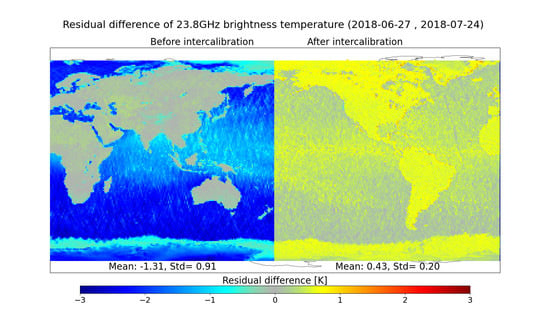
Figure 11 presents the residual differences between S3A and S3B brightness temperatures for the cycle 10 of S3B, averaged in boxes of 2${}^{\circ }$× 2${}^{\circ }$. The 23.8 GHz/36.5 GHz global biases are equal to −1.3 K/−0.7 K respectively, meaning that S3B measurements are colder than S3A. However, the bias is characterized by a scene dependency as shown by the maps of Figure 11 and also by the histograms of Figure 12a. The latter reveals a bi-modal structure for both channels. A first mode has an average bias close to zero, corresponding to the measurements over land. The second mode has an average bias close to −2 K corresponding to the ocean measurements. The two modes are more clearly defined for the 23.8 GHz channels than for the 36.5 GHz, because the difference between S3A and S3B over ocean is larger for this frequency.

The method used for S3A was employed for S3B calibration, i.e., the update of a set of characterisation parameters, with a correction within the range of the measurement uncertainty of each parameter. The target for the final set of characterisation parameters are the reduction of the residuals as well as the vicarious calibration consistency. The in-house prototype is used to compute brightness temperatures with the new set of parameters, that will be subject to review with the same diagnosis as for the first assessment. Results are presented in Figure 13 for the map of the residuals and Figure 12b for the histograms. One can see the biases are clearly reduced between the two instruments. It subsists a bias of 0.4 K for the 23.8 GHz channel and 0.2 K for the 36.5 GHz. A scene dependency is still observed but of much smaller amplitude. The standard deviation of the residuals are 0.56 K and 0.65 K for channels 23.8 GHz and 36.5 GHz respectively. The expected value can be estimated using the noise of the two instruments equal to 0.29 K/0.31 K for 23.8 GHz channels and 0.31 K/0.32 K for 36.5 GHz channel of S3A/S3B respectively. Thus the theoretical standard deviations of the S3A/S3B differences are equal to 0.42 K/0.45 K for 23.8 GHz/36.5 GHz respectively, very close to the results observed on the residuals.

4. Geophysical Products Performances

4.1. A Neural Network Retrieval Approach

The retrieval approach used for Sentinel-3 is based on a neural network architecture. Surface and profiles parameters from ECMWF analyses are extracted at 12AM for one day for each month of a chosen year, on a 0.5${}^{\circ }$× 0.5${}^{\circ }$ grid. UCL radiative transfer model [19,20] is used to compute simulated brightness temperatures and altimeter backscattering coefficient. The database is composed of the simulations and the reference parameters to be retrieved, computed from the ECMWF profiles. The database is randomly split in two, with a repartition of 20% and 80% respectively for the learning database and the test database. The neural network consists in one hidden layer of eight neurons. The activation function is a sigmoïd function, and the transfer functions of the hidden and output layer are a weighted sum of the inputs. Inputs and reference are normalized to provide the neural network inputs with similar scales.

The critical points of the learning process are the accurate description of the surface and the atmospheric properties, the representativeness of the database, and the correlation between the inputs (brightness temperatures) and the reference parameters like the wet troposphere correction. The latter explains why retrieval algorithms based on simulations have better performances than empirical algorithms. It means also that a transfer function between real measurements and simulations is required to achieve the best performances. While the learning can be performed before launch, this transfer function can be only be estimated after launch using real measurements.

The measured-to-simulated brightness temperatures transfer function is a linear function estimated through an iterative processing. The initial relation is provided by the linear fit on the scatterplot of measurements and simulations. The co-locations are looked for in a time/space window of ±50 km/±30 min. An editing is required to filter out all the cases where the observation and the model estimation are not consistent. We use the same filtering as in the single difference estimation in the previous section, consisting in thresholds in distance to shoreline, difference of the brightness temperatures, and difference of cloud liquid water content. Starting from this initial state, iterations are performed over the slope and bias for the two brightness temperatures. At each iteration, the difference between the retrieved wet troposphere correction and the correction estimated from ECMWF data is estimated (hereafter called D_tropo) as well as difference of variance of SSH at crossover points. The final set of values is chosen to fulfill all the following criteria:

• The mean value of the D_tropo shall be smaller to 1cm. The shape of histogram is also considered and shall be close to a gaussian distribution.
• The difference of variance of SSH at crossover points shall be minimal.

Finally, this process provided the following set of values in

Table 3. Measured-to-simulated brightness temperatures transfer function.

	Slope	Intercept
23.8 GHz	1.015	−3.5
36.5 GHz	1.03	−4

for the two channels of the MWR.

Two different retrieval algorithms are used for Sentinel-3 processing. The first one is a 3-inputs algorithm (called 3P), using the two brightness temperatures from the MWR and the altimeter backscattering coefficient (${\sigma }_0$). 3P algorithms have been designed to retrieve the four geophysical parameters: wet troposphere correction (WTC), atmospheric attenuation for the sigma0, water vapor content, cloud liquid water content. Following Envisat heritage [21], an advanced algorithm, called 5P has also been developed for the retrieval of the WTC using two additional parameters: the sea surface temperature and the atmospheric lapse rate. The Sea Surface Temperature brings information from the surface temperature not provided by the Sigma0. The temperature lapse rate improves the retrieval in areas of specific temperature profiles like the upwelling regions. Each of these algorithms has its own set of weights and biases, but the adjustment function is the same.

4.2. Assessment of Wet Troposphere Correction

The wet troposphere correction (WTC) retrieved from MWR measurements is compared to several missions corrections. As these missions have different characteristics such as inclination and local time, a proxy for their comparison is the model correction computed from profiles and surface parameters provided by ECMWF analyses. Four analyses per day are used, and bilinear interpolation in space and time is performed to compute a model correction co-located to the measurements. Details on this comparison can be obtained in the S3 MPC related paper [15] or the cyclic reports available online on ESA website [22].

The analyse of crossover points between two missions is another proxy to achieve comparison and results are shown in Section 4.2.2. Finally geophysical assessment is performed by analysis of the difference of variance of Sea Surface Height at crossover points in Section 4.2.3. MWR correction for each mission is compared to the ECMWF correction at crossover points, and missions can be compared by their improvement with respect to the model.

4.2.1. Data Overview

Data required for the analyses described earlier are listed hereafter. S3A wet troposphere corrections are provided in operational Level-2 products in four variables: solutions are available for SAR and PLRM ${\sigma }_0$, for both 3P and 5P algorithms. Jason-3 data are extracted from Level-2 GDR-E products, computed using the three brightness temperatures. AltiKa data from Level-2 GDR-E products. A reprocessing in GDR-F standards with enhanced algorithm is on-going; but a long-enough time series of data in this standard was unavailable at the time of writing this paper. Details can be found in Section 3.3.1. Data coverage for each dataset is provided in

Table 4. Data coverage for crossover and variance of Sea Surface Height (SSH) analyses.

	AltiKa	Jason-3	S3A	S3B
coverage	cycle 32 to 134	cycle 6 to 153	cycle 3 to 58	Cycle 20 to 38
date	March 2016 to Nov 2019	April 2016 to April 2020	April 2016 to May 2020	January 2019 to May 2020

.

4.2.2. Comparison at Crossover Points

The reference mission for multi-mission crossover points is Jason-3. Indeed, due to its orbit inclination of 66${}^{\circ }$, the crossover points will be located more homogeneously over the globe, and not only in the high latitudes. As the atmosphere is varying very quickly, the time criteria shall be as short as possible, within the temporal correlation of the WTC. The time lapse is set to one hour. All weather conditions are considered, no specific filtering on clouds is applied but we used the validity criteria as defined by the CalVal team. As we aim to compare wet troposphere correction, we will consider only ocean measurements. Hence, a distance to shoreline criteria (>50 km) is applied to remove land contamination issue. Finally only latitudes below ±60${}^{\circ }$ are considered. For the comparison of Jason-3 with S3A and AltiKa, the period of study covers from the year 2016 up to 2020.

Figure 14 presents monthly average of the difference of WTC (PLRM 3P and 5P) at cross-over points of S3A and Jason-3 (Figure 14a), AltiKa (Figure 14d), and S3B (Figure 14c) with Jason-3. Boxes on these figures represent the limit of the lower and upper quartiles; white lines in the boxes are for the median values, and the whiskers the 5th and 95th percentiles.

Figure 15 illustrates the localisation of these points for both couples of instruments (S3A/J3 and AL/J3). Right panels of Figure 15 provide statistics per 2${}^{\circ }$ of latitude bins: the number of points is shown in blue points, the average per bin in full orange line, and standard deviation in orange dotted line. One can see that the crossover points are globally distributed over the ocean. Southern high latitudes count a higher density of points due to larger ocean fraction in the south hemisphere, but we still have a significant number of points in the equatorial and northern hemisphere. We notice an average bias of −0.55 cm between S3A and Jason-3 and close to zero (−0.06 cm) for AltiKa. These results are consistent with the multi-mission monitoring of D_Tropo (MWR-ECMWF difference) presented in [15] or [22]. The bin averaged values present a V-shape, with lower differences in the equatorial band and higher differences in the highest latitudes. The amplitude of this signal is larger for AltiKa than for S3A. This kind of signal has already been observed with AltiKa and Metop-A with respect to Jason-2 [23,24] on the 23.8 GHz brightness temperatures. It is thus not surprising to find it on the comparison between S3A and Jason-3, since Jason-3 has been calibrated with Jason-2 as a reference. The standard deviation is slightly larger for AltiKa (0.96 cm) than for S3A (0.78 cm).

Monthly average of the difference of WTC at crossover points presents a drift of 0.05 cm per year over the 4-years period for S3A vs. Jason-3 (Figure 14). Slope estimation is similar for the PLRM 5P WTC for S3A (Figure 14b), with a slightly larger bias and similar standard deviation. The estimated slope is a little larger for AltiKa versus Jason-3 (Figure 14d), estimated to 0.08 cm per year. Data up to November 2019 only are used for this estimation, in order to prevent impact from processing updates. Indeed, since December 2019, AltiKa processing is running on GDR-F standards and a major update of the wet troposphere correction is included in this new version. One can observe the impact on the comparison with Jason-3: the monthly standard deviation since December 2019 is clearly reduced with respect to the previous months. Estimated drifts estimated from the S3A and AltiKa with respect to Jason-3 are consistent and very small. However, a 4-years time-window is quite short to estimate such drift with a high confidence. S3B is also compared to Jason-3 (Figure 14c). First statistics are similar to S3A/J3 results, if first cycles are unconsidered as the MWR was yet uncalibrated. However, as the time series is naturally much shorter, a drift is not yet estimated for this instrument.

4.2.3. Gain on The SSH Variance At Cross-Overs

Performances of the retrieval algorithm over ocean are assessed through the Sea Surface Height and more precisely through the criteria of difference of variance of SSH at crossover points. This diagnosis makes the assumption that the ocean height does not change significantly within a 10-days window. Thus, the variability observed is caused by the corrections, that do not precisely match the reality. When comparing two solutions, a reduction of the variance with one of the solution indicates the best one. When several missions need to be compared, the natural proxy is the model correction, as it can be computed for each mono-mission crossover points. Figure 16 provides the quantitative improvement by employing MWR solutions with respect to ECMWF solution, and geographical patterns are shown in Figure 17.

Performances are estimated for valid crossover points according to the validity criteria defined by the CalVal team, annotated “Global”, and for low ocean variability selection annotated “low var”. All the MWR-based solutions are reducing the variance with respect to the ECMWF solution, indicating an improvement with MWR solutions. Jason-3 provides the best performances with an improvement of −1.86 cm² and −2.37 cm² respectively for global and low variability selections. This is expected as Jason-3 embarks a three-channel radiometer and benefits from the additional 18.7 GHz frequency sensitive to wind-induced effect on surface emission and surface temperature. S3A solutions using PLRM ${\sigma }_0$ produce better performances than the ones using SAR ${\sigma }_0$: −1.39 cm² and −1.49 cm² for respectively 3P and 5P algorithms using PLRM ${\sigma }_0$, while using SAR ${\sigma }_0$, is it of −1.15 cm² and −1.32 cm² for respectively 3P and 5P algorithms. This result is not fully explained yet. It may be induced by a scale inconsistency between SAR ${\sigma }_0$ and MWR measurements. Moreover, simulated ${\sigma }_0$ in the learning database of the neural network may be closer to the PLRM ${\sigma }_0$. Regarding the 3P and 5P algorithms, the latter brings an improvement of −0.1 cm². This improvement is smaller than anticipated, considering results shown in previous studies such as [4]. AltiKa results are also presented for two different algorithms, one using three parameters (Patch2) [4], the other using five parameters (Patch3). However, these two algorithms cannot be compared directly as they are dissimilar in conception. The so-called Patch2 is an algorithm based on a simulated database, but with known flaws due to the simulated ${\sigma }_0$ in Ka band. The so-called Patch3 is an empirical algorithm using measurements in the learning database. The performances of the Patch2 are lower than the same type of algorithm for a Ku ${\sigma }_0$. We can notice that S3A PLRM 5P solution have performances similar to AltiKa Patch3. S3B performances are similar to S3A (Figure 16) although the period of study is shorter, leading to a noisier map (Figure 17b).

S3A and S3B performances are satisfying the expectations according to the diagnosis presented here, and fulfilling the mission requirements. A new algorithm for S3A and S3B will be developed in 2020 by S3 MPC that may improve the 5P retrieval.

5. Conclusions

Sentinel-3 Microwave radiometers complement the altimeter allowing the estimation of the excess wet path delay due to the presence of water vapor in the atmosphere. Their identical design includes two near-nadir channels and a noise injection technology. The internal calibration is performed using an internal hot load and a sky horn.

The in-flight calibration of S3A has been performed using vicarious calibration and comparison to other instruments, by updating a set of characterisation parameters, the initial vector being the on-ground characterisation. The tandem phase between S3A and S3B have been a significant asset for the inter-calibration. The flight configuration with only 30 s between the instruments measurements is ideal to assume that both instruments have observed the same atmosphere. S3B and S3A are inter-calibrated within 0.4 K/0.2 K for 23.8 GHz/36.5 GHz channel. A slight scene dependency is still observed for the first frequency channel.

Wet troposphere correction is retrieved using several algorithms for S3A and S3B. The 5P algorithm provides better performances than the 3P algorithm, as expected, and is performing very well. However, the improvement between 5P and 3P is expected to be larger. A new algorithm is in preparation that will provide the expected performances.