Multi-Source Remote Sensing Data Product Analysis: Investigating Anthropogenic and Naturogenic Impacts on Mangroves in Southeast Asia

Abstract

This study investigated the drivers of degradation in Southeast Asian mangroves through multi-source remote sensing data products. The degradation drivers that affect approximately half of this area are unidentified; therefore, naturogenic and anthropogenic impacts on these mangroves were studied. Various global land cover (GLC) products were harmonized and examined to identify major anthropogenic changes affecting mangrove habitats. To investigate the naturogenic factors, the impact of the water balance was evaluated using the Normalized Difference Vegetation Index (NDVI), and evapotranspiration and precipitation data. Vegetation indices’ response in deforested mangrove regions depends significantly on the type of drivers. A trend analysis and break point detection of percentage of tree cover (PTC), percentage of non-tree vegetation (PNTV), and percentage of non-vegetation (PNV) datasets can aid in measuring, estimating, and tracing the drivers of change. The assimilation of GLC products suggests that agriculture and fisheries are the predominant drivers of mangrove degradation. The relationship between water balance and degradation shows that naturogenic drivers have a wider impact than anthropogenic drivers, and degradation in particular regions is likely to be a result of the accumulation of various drivers. In large-scale studies, remote sensing data products could be integrated as a remarkably powerful instrument in assisting evidence-based policy making.

1. Introduction

Mangroves are woody plants located in the intertidal areas of tropical and subtropical regions. They typically thrive under harsh environmental conditions, such as high salinity, high temperature, extreme tides, and high sedimentation [1,2]. These productive and biologically important ecosystems provide crucial protection for coastal and marine systems, as well as humans, such as preventing abrasion [3], reducing tsunami impacts [4], providing an ecosystem for flora and fauna [5], and acting as a sink for carbon dioxide [6].

In Southeast Asia, mangrove forests cover an area of 63.2 × 105 ha, which constitutes 34.9% of the area of the world’s mangrove forests (181.1 × 105 ha), with great species richness and structure [7,8]. The depletion rate of Southeast Asian mangroves from 2000 to 2012 was 4.73%, which amounts to an annual global loss of 0.39% [9]. Because of this depletion, mangrove forests are facing considerable risks [10,11]. This depletion is due to both anthropogenic and natural changes [12]. In terms of anthropogenic drivers, a significant proportion of mangrove loss is caused by the direct destruction of these forests for other land uses. These include overexploitation by coastal communities; conversion to settlements, tourist resorts, and agricultural land for rice, coconut fields, salt bed, industrial activities, and brackish-water aquaculture [13]. Natural drivers such as climate change, accelerated sea-level rise, meteorological phenomena, a changing water balance, and other aspects of global change also affect mangrove forests across the world [14]. Natural drivers of mangrove loss were frequently observed and widely distributed across the globe [15,16,17]. However, natural drivers constitute a substantial proportion of predicted future losses, primarily due to changes in meteorological phenomena [18,19], which can reduce precipitation levels and increase evapotranspiration [20], affecting the water balance that is vital for healthy mangrove forest growth.

Vegetation, soil, and water are interrelated factors that influence mangrove life. Soil has many functions that are very important for mangrove growth; for instance, each mangrove species requires a different type of soil texture to live [20,21,22,23]. Changes in soil characteristics can affect the capacity of mangroves to capture carbon [24,25]. In addition, soil factors can also affect vegetation. For example, changes in nutrient content in the soil can cause competition between mangroves and other vegetation, resulting in changes in vegetation zone [26,27]. Another factor that greatly influences mangrove life is water. Mangroves can only survive in tidal inundation with a range of 0.4–1.27 m [28,29]. Increases in sea level due to climate change will cause mangroves to die and the surrounding area to be no longer suitable for planting mangroves [30,31].

Changes in vegetation, water, and soil are often detected using indices such as the Normalized Difference Vegetation Index (NDVI), the Normalized Difference Water Index (NDWI), and the Soil Adjusted Vegetation Index (SAVI). A study by Gupta et al. [32] used NDVI and NDWI to distinguish mangrove and non-mangrove forests by looking at the greenness index and water content of the vegetation, which were then compared with SAVI and Simple Ratio (SR). Meanwhile, Ahmed et al. [33] detected changes in land cover from mangrove areas to water areas in the southwestern coastal areas of Bangladesh that were flooded using NDVI and NDWI. Another example is the study by Pastor-Guzman, [34], in which the phenology of mangrove forests was investigated with the Enhanced Vegetation Index (EVI), NDVI, the Green Normalized Vegetation Index (GNDVI), and NDWI.

Another developing research area, land use and land cover (LULC) change, has emphasized the generation of global land cover (GLC) products from numerous observation satellites as primary data for both global or national scale studies [35,36]. Presently, these accessible GLC products have been widely utilized through an aggregation in several research topics, including estimating agricultural enlargement into forests [37], monitoring cropland changes [38], and deriving user-specific maps [39]. In the context of mangroves, Hamilton and Casey [9] successfully integrated MFW [40] as the basis of mangrove area, world ecosystem, namely ecoregion layer, and GFC [41], namely annual forest change data, to produce global mangrove forest cover data from 2000 to 2012. This proves that the assimilation of global data products, mainly GLC products processed through robust and standardized methodology, has great potential to be addressed in investigating mangroves drivers over a large region.

Future climate models consistently increased variability in temperature and extreme precipitation [42]. According to Bathiany et al. [43], temperatures increased by 10% C⁻¹ in Southeast Asia with the mechanism of soil drying and shifting of atmospheric structures. An increase in temperature will result in an increase in water loss during the evapotranspiration process [44], in turn impacting water availability for plants. According to Maslin and Austin [45], changes in the predicted total annual precipitation are very diverse and difficult to ascertain. However, according to Myhre et al. [46], precipitation will continue to increase almost twofold for any further global warming. An increase in rainfall will cause plants to die [47]. These studies indicate that an increase in temperature and extreme precipitation could be one of the reasons for the occurrence of naturogenic deforestation. Therefore, it is necessary for there to be a study related to water balance in order to determine the effect of climate change on water content in mangrove vegetation.

Remote sensing has been widely used for forest monitoring, and such multi-temporal change detection with high spatial and temporal resolution data can be used to monitor meteorological phenomena that affect water balance [48,49]. An index of mangrove forests derived from satellite imagery can be used to assess coastal impacts over large areas [50]. However, to diminish the degradation of mangrove forests, coastal areas must also be constantly monitored. However, this presents challenges to current remote sensing techniques [51]. Several studies have been conducted to monitor deforestation and degradation in mangrove forests using remote sensing and geographic information system (GIS) analysis [9,10,11,52]. Hamilton and Casey [9] used several global database maps to estimate the annual global mangrove forest change from 2000 to 2012. Richards and Friess [10] combined remote sensing and GIS techniques to quantify the proximate drivers of mangrove deforestation in Southeast Asia by identifying the dominant land use and land cover area that replaced the areas of deforested mangroves between 2000 and 2012, which they summarized in a one-degree spatial resolution dataset. Those data products were then improved by Fauzi et al. [52], who analyzed environmental and socio-economic data products to identify anthropogenic mangrove forest deforestation drivers in a finer resolution of 10 km grid cells. However, the results of the study show that the drivers in a high percentage of deforested mangrove areas were unidentified. This has raised the question as to whether there are contributing factors to mangrove deforestation other than land conversion, because none of the previous studies used remote sensing data products to identify both anthropogenic and naturogenic drivers of mangrove deforestation in Southeast Asia.

The main objective of this study is to identify mangrove forest areas that have been degraded and depleted due to anthropogenic and naturogenic factors. For the anthropogenic analysis, various data products of global land cover (GLC) were compared and then integrated in order to monitor mangrove deforestation in Southeast Asia. We also determined the spatiotemporal trends of remote sensing vegetation indices over the land use and land cover (LULC) conversion of mangrove forests in Southeast Asia, and characterized the relationship between vegetation indices and mangrove deforestation drivers. For the analysis of natural drivers, the effects of water balance on mangrove forests’ degradation and depletion were identified. Mangrove forests’ degradation and depletion must also be affected by the water balance of each species of the mangrove itself. Therefore, this research analyzed how the water balance in mangroves affected the degradation of the mangrove forests. Thus, adaptation options to avoid and minimize mangrove depletion can be identified and implemented. To the best of our knowledge, this is the first study to investigate both naturogenic and anthropogenic impacts on mangrove deforestation in Southeast Asia, by integrating the available multi-source remote sensing data products. We also attempted to develop a novel algorithm for the mangrove water balance model. Moreover, the method applied in the consistency assessment step can be adopted to evaluate the accuracy of result involving similar topics. The remainder of this article is presented in four sections detailing the materials and methods, results, discussion, and conclusion. In Section 2, we specified the type, spatial and temporal resolution, source, and characteristics of the data we used to analyze mangroves, land use, land cover, and remote sensing data products. In this section, we described the general framework of this study and detailed the methods used to process the collected data. In Section 3, we presented our findings by showing the MODIS vegetation indices’ response for specific mangrove areas, the estimated land cover conversion of mangrove area based on GLC data products integration, and the mangrove coefficient growth, and identified the water balance in the mangrove areas. In Section 4, we reviewed the conformity of data products with Dominant Land Use of Deforested Mangrove Patches (DLUDMP) and The Southeast Asian Mangroves Conversion Types (SEAMCT) and the uncertainties associated with the mangrove variation data. We also present a trend analysis and breakpoint detection in particular deforested mangrove areas and future research directions. In Section 5, we summarized our findings, highlighted the strengths and limitations of this study, and elaborated on areas of further research.

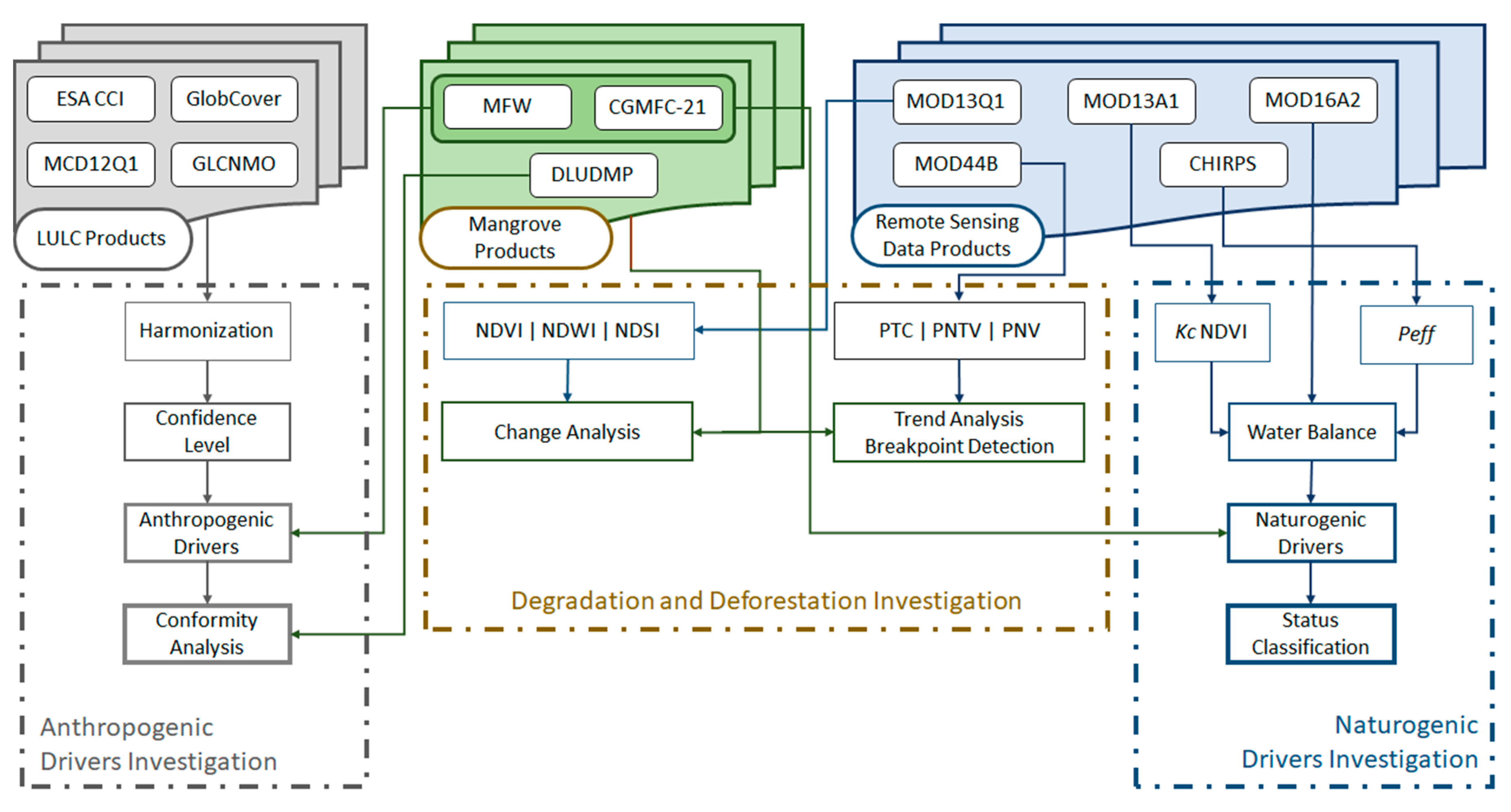
2. Materials and Methods

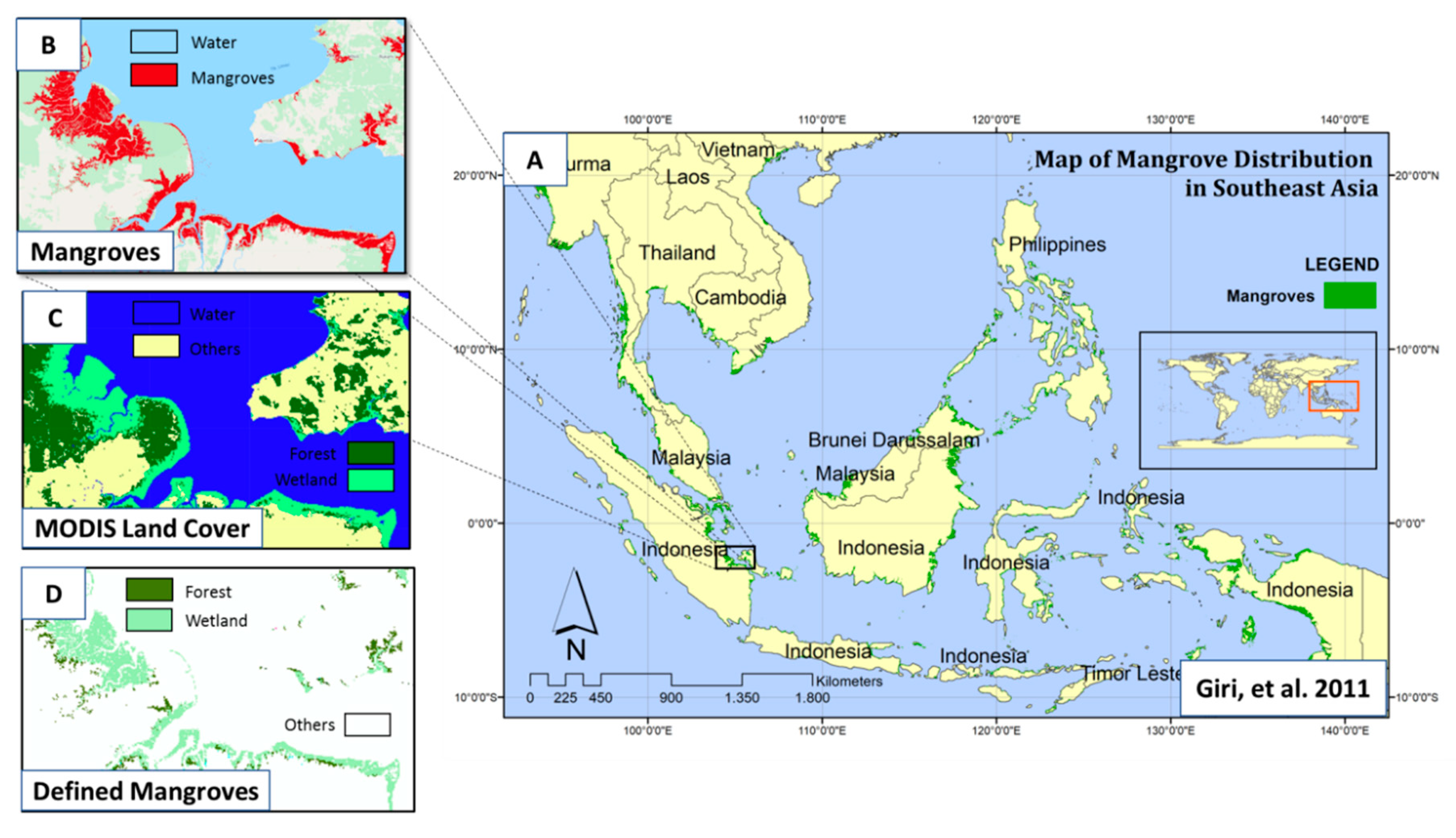
2.1. Data Used in This Study

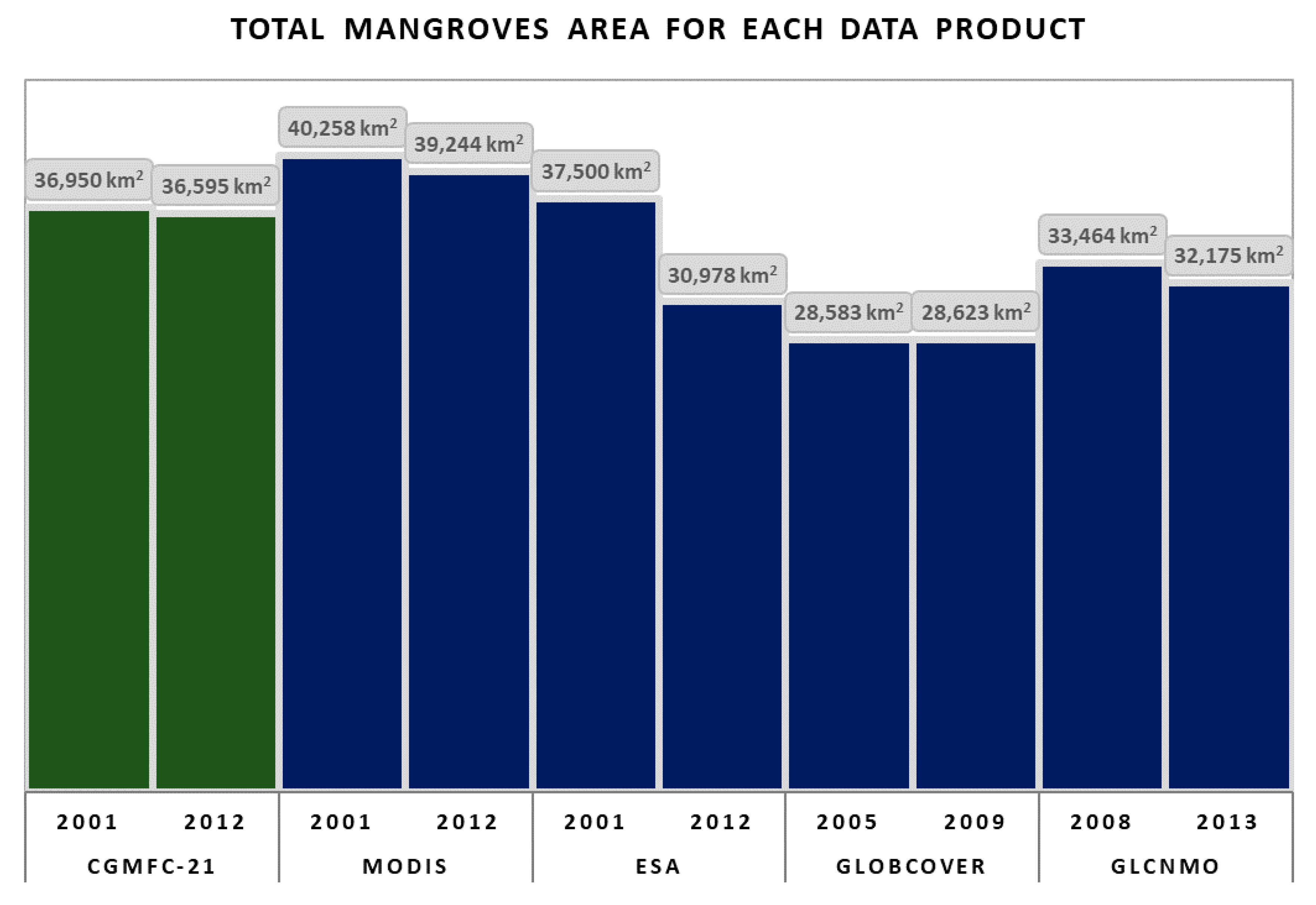
2.1.1. Mangrove Data Product and Change

This study used several data products produced from previous studies regarding mangrove distribution and deforestation to provide an improved spatiotemporal analysis (

Table 1. Product specifications of mangrove data and their change.

Data Product	Data Class	Spatial Resolution	Available Year	Source
MFW-USGS	Mangrove Distribution	30 m	1997–2000	[40]
CGMFC-21	Mangrove deforestation	30 m	2001, 2005, 2009, and 2012	[9]
DLUDMP	Function of dominant land	1°	2012	[10]
SEAMCT	Mangroves Conversion Types	10 km	2000 and 2012	[52]

).

The Global Distribution of Mangroves (MFW) [40] is the primary data produced from the Landsat satellite image with a spatial resolution of 30 m obtained from 1997 to 2000, while the secondary data are based on the database of global, national, and local mangrove forests.

The accuracy of this product was validated by dividing the whole area into 500 × 500 grids. Each grid was qualitatively controlled in virtue of the local experts and very high-resolution images, i.e., QuickBird and IKONOS [40]. In addition to the mangrove’s maps existence, although some mangroves distribution data are available, i.e., Spalding et al. [53], Saputro et al. [54], and Bunting et al. [55], we decided to only use MFW owing to the year of the existence i.e., 2000, which is more appropriate in performing long-term evaluation. Nonetheless, those mangrove datasets were processed in providing the agreement level analysis.

The Global Database of Continuous Mangrove Forest Cover for the 21st Century (CGMFC-21) [9] was produced by combining the Global Forest Change (GFC) [41], MFW [40], and the Terrestrial Ecosystem of the World (TEOW) [56] databases, as well as other data, to produce annual global mangrove forest cover maps from 2000 to 2012 with a spatial resolution of up to 30 m. The Dominant Land Use of Deforested Mangrove Patches (DLUDMP) [10] data product, compiled in 2012, presents information about the function of the dominant land in the area of deforested mangroves, with a spatial resolution of one degree. The function of dominant land is determined by estimating the largest land function range in the area of deforested mangroves, which is then indicated as the land function causing mangrove conversion. The Southeast Asian Mangroves Conversion Types (SEAMCT) by Fauzi et al. [52] was produced from environmental data products, i.e., MFW, CGMFC-21 [9], MODIS Land Cover Type Product (MCD12Q1) [57], Global MODIS Water Maps Version 6 (MOD44W) [58], Global Human Settlement (GHS) [59], and History Database of the Global Environment Version 3.2 (HYDE 3.2) [60], and socio-economic data, i.e., Defense Meteorological Satellite Program–Operational Linescan System (DMSP–OLS) [61], Gross Domestic Product (GDP) [62], and Gridded Population of the World Version 4 (GPW) [63], to provide an enhanced mangrove forest deforestation driver map from 2000 to 2012 with a 10 km spatial resolution. This data product presents detailed information on anthropogenic deforestation drivers based on the dominant land cover changes, which were classified as conversion to agriculture, aquaculture, infrastructure, or other human activity, as well as a combination of these factors.

2.1.2. Land Use Land Cover Data Products

To identify land conversion from mangrove forest area to other land cover types, several GLC data products were used (

Table 2. Product specification of global land cover (GLC) datasets.

Data Product	Data Class	Spatial Resolution	Data Acquisition	Source
ESA CCI Land Cover	Land cover	300 m	2001 and 2012	[64]
MCD12Q1	Land cover	500 m	2001 and 2012	[65]
GlobCover	Land cover	300 m	2005 and 2009	[66]
GLCNMO2008	Land cover	500 m	2008 and 2012	[68,69]

). These databases provide adequate spatiotemporal resolution produced from various remote sensing data. The European Space Agency (ESA) CCI Land Cover [64] product was compiled from 1992 to 2015 with a spatial resolution of approximately 300 m or lower and produced through combined classification (guided and unguided) of multi-spectral data from MERIS obtained from 2003 to 2012. Such data are processed using guided and unguided classification algorithms combined automatically to obtain different land cover classes. The MODIS Land Cover Type (MCD12Q1) [65] data product was produced using guided classification of Terra and Aqua MODIS to produce annual GLC from 2001 to 2012 with a spatial resolution of 500 m. These data function as early warning indicators of GLC change. The main classes of land cover are vegetation (11 classes), land (3 classes), and non-vegetated land (3 classes). The GlobCover Global data product [66] is produced through an annual mosaic obtained from the MERIS inventory with a resolution of 300 m through the ENVISAT instrument [67]. The first product of GlobCover was produced in 2005 by the ESA in collaboration with international networks, including the Environmental Agency (EEA), United Nations Environment Program, Global Observation of Forest Cover and Land Dynamic (GOFC-GOLD), Joint Research Centre, and International Geosphere-Biosphere Programme (IGBP). The Global Land Cover by National Mapping Organizations (GLCNMO2008) [68,69] was produced through a global mapping project conducted by an international steering committee on global mapping. Version 2 of this dataset was based on 16 days of MODIS data (MCD43A4) from 2008, with a spatial resolution of 500 m due to the two directional reflectance distribution function (BDRF), with an overall accuracy of 77.9%.

2.1.3. Geophysical and Vegetation Parameter Products from Remotely Sensed Data

In addition to the processed data provided by the previous studies, other remote sensing datasets were used to obtain temporal environmental information. The specifications of the remote sensing datasets used in this study are summarized below in

Table 3. Product specification of remote sensing datasets.

Data Product	Data Class	Spatial Resolution	Temporal Resolution	Source
MOD13Q1 v006	VI and SR	250 m	2000 and 2012	[70]
MOD13A1 v006	Vegetation Indices	500 m	2002 and 2012	[71]
MOD16A2 v005	Evapotranspiration	500 m	2002 and 2012	[75]
CHIRPS v02	Precipitation	~5.3 km	2002 and 2012	[79]
MOD44B v6	PTC, PNTV, PNV	250 m	2000–2013	[80]

. The MOD13Q1 Version 6 product [70] provides a vegetation index (VI) value per pixel basis at a 250 m spatial resolution. There are two primary vegetation layers (NDVI and EVI). The MODIS Vegetation Indices (MOD13A1 v06) Version 6 product [70] provides VI values at a per pixel basis at a 500 m spatial resolution. The two primary vegetation layers improved the sensitivity of the MODI3QI and the MOD13A1 datasets over high biomass regions such as the equatorial area of Central Africa, South America, and Southeast Asia [71,72]. This improvement is important because the vegetation index is prone to saturation on high biomass due to the optical signal not being able penetrate the highly dense canopy [73,74]. The MODIS Global Terrestrial Evapotranspiration (MOD16A2 v05) [75] is a monthly composite dataset produced at a 5 km pixel resolution to estimate the global terrestrial evapotranspiration. The MOD16 global evapotranspiration product can be used to calculate the water and energy balance and the soil water status at a regional scale, providing key information for water resource management. The Climate Hazards Group InfraRed Precipitation with Stations (CHIRPS v02) dataset [76] is a blended product combining pentadal precipitation climatology and quasi-global geostationary thermal infrared satellite observations from the Climate Prediction Center (CPC), and the National Climatic Data Center (NCDC) [77] atmospheric model rainfall fields from the NOAA Climate Forecast System version 2 (CFSv2) [78] and in situ precipitation observations. These data are used because CHIRPS is an in situ station dataset used to create a gridded rainfall time series for trend analysis and seasonal drought monitoring [79]. The MOD44B Version 6 Vegetation Continuous Fields (MOD44B) [80] presents sub-pixel information about the characteristics of worldwide vegetation cover classified into three classes: percentage of tree cover (PTC), percentage of non-tree vegetation (PNTV), and percentage of non-vegetation (PNV), with a 250 m spatial resolution.

2.2. Methodology

This study was divided into three main parts: the investigation of degradation and deforestation, anthropogenic drivers, and naturogenic drivers, as demonstrated in Figure 1. To investigate anthropogenic drivers, we examined the ESA CCI, GlobCover, MCD12Q1, and GLCNMO data products to estimate major LULC change in mangrove areas. Previous studies revealed LULC changes as the dominant driver of mangroves deforestation [10,11,52]. In this research, we exploited the available GLC products commonly used to identify human disturbances over Southeast Asian mangroves. Although these data products were produced based on reliable procedures, we believe that there is no perfect product. Therefore, we used all the available GLC products to improve the sensitivity of the results that were then presented through the level of agreement. The level of agreement can also help us understand how these data are related to each other. Since each product defines mangrove forests differently and refers to a different classification system, the main challenges in comparing land cover was the reconciliation of the type of land cover class [81,82]. This was done at the beginning of the process, then the obtained results were compared with those of other studies.

When investigating deforestation and degradation, we employed MOD13Q1 and MOD44B to analyze mangrove loss from 2000 to 2012. As mangrove ecosystems are inundated land that consist of vegetation, water, and soil, we explored three types of commonly used vegetation indices in mangrove studies that represent each component: NDVI, NDWI, and SAVI [32,83,84]. The derived and calculated vegetation indices from the 16 day MOD13Q1 data, annual NDVI, NDWI, and SAVI were calculated to highlight the differences of each index over the 12 years in specific regions. Other indices were identified and traced by annual PTC, PNTV, and PNV (MOD44B) datasets from 2000 to 2013, using trend analysis and breakpoint detection [85] to identify the dynamic patterns and the exact years of particular land use expansion. The trendline slope was calculated by the least-squares-based linear regression method, while the breakpoints were identified using the Bai and Perron method [86,87]. Then, we considered using high resolution imagery to validate our findings.

To investigate the naturogenic drivers, we focused on the impact of water balance on the mangrove ecosystem. For data analysis and synthesis, linear regression models that establish the relationship between the vegetation index and mangrove coefficient growth were used as a proxy for the mangrove growth coefficient. Since mangroves are highly sensitive to changes in their water supply, the water balance model was used represent the natural drivers [88,89]. The water balance within an area can also reflect primary climatic parameters, e.g., precipitation, evapotranspiration, and temperature analysis. This model can also be used to identify the potential drought impact within mangrove ecosystems due to ongoing global climate change. The mangroves’ water balance was quantified by multiplying the mangrove growth coefficient, calculated using NDVI (MOD13A1) data, by the evapotranspiration (MOD16A2) data, and then subtracting the precipitation (CHIRPS) data from it. The result of this process has a 500 m grid size. The spatial resolution was decided by considering the most common spatial resolution of the datasets and of the coverage of the study area. Specifically, we upscaled the lower resolution datasets and downscaled the higher resolution ones through resampling based on the bicubic interpolation method. To validate the results, the relationships between the mangrove’s water balance and degradation and depletion were analyzed.

In this study, we tried to explore all available data products with various spatial resolution and time acquisition to reach maximal outcome. In combining multi-resolution data products, the resampling must be applied to uniform those datasets. Based on recent research articles, there are diverse approaches used to decide the basis of the grids size for the resampling result including the coarser spatial resolution among datasets [90], the modus or the most spatial resolution on the input data [91,92], the mean spatial resolution [93], and the specific resolution based on other referred data [94,95]. In this case, we assumed that there is no certain procedure to be adopted in achieving ideal spatial resolution for assorted topics. Thus, in this study, we consider the most spatial resolution and characteristic of parameters represented for each dataset (e.g., high spatial resolution is not necessary for precipitation) as the basis of the resampling result, i.e., 500-m spatial resolution. On the other hand, considering different time acquisition issues could affect the consistency of the product, we conducted agreement level analysis in the discussion as carried out by a similar research approach [96,97,98]. This analysis is commonly adopted by overlaying all datasets to assess the accuracy and inconsistency among these data [96,99,100].

2.2.1. Harmonization of Land Cover Data Product

In the first step, to harmonize the type of land cover data from various land cover products, the data were separated into two new classes. The first class was considered mangrove forest (

Table 4. Classes of each land cover product defined in the “mangrove forest” class.

Land Cover Product	Class	Description	Classification Reference
ESA CCI Land Cover	Forest	Trees with large and/or pointy greenish and yellowish leaves, open or closed alongside bush and grass, which have a canopy cover of 15% and over.	Land Cover Classification System (LCCS)
	Wetland	Trees inundated with fresh water or sea water, mixed in with the bush or grass
GlobCover	Forest	Trees with large leaves and/or pointy greenish or yellowish leaves, open or closed with a height of 5 m, mixed in with other vegetation, such as bush and grass, with a minimum canopy cover of 15–40%.	Land Cover Classification System (LCCS) from FAO
	Wetland	Vegetation (Grass, Bush, Wood Vegetation), open and closed, inundated by fresh or sea water (>15%).
MODIS Land Cover	Forest	Trees with large or pointy leaves, greenish or yellowish, with a height of more than 2 m and a canopy cover of more than 60%.	International Geosphere-Biosphere Programme (IGBP) Legend and Class
	Wetland	Land where 30–60% of its area is permanently inundated with fresh water or seawater, covered by at least 10% from other vegetation.
GLCNMO	Mangrove	-	Land Cover Classification System (LCCS) from FAO

), and the second class was considered the land cover causing mangrove deforestation (

Table 5. Estimation of each type of land cover conversion in mangrove forest areas.

Land Cover Product	Early Land Cover Class	Ultimate Land Cover Class	Type of Conversion of Land Cover from Mangrove Deforestation
ESA CCI Land Cover, MODIS Land Cover, and GlobCover	Forest	Agriculture	Mangrove to farming
		Wetlands	Mangrove to fishery
		Water	Mangrove to fishery
		Urban	Mangrove to housing
	Wetlands	Agriculture	Mangrove to farming
		Water	Mangrove to fishery
		Urban	Mangrove to housing
GLCNMO	Mangrove	Agriculture	Mangrove to farming
		Wetlands	Mangrove to fishery
		Water	Mangrove to fishery
		Urban	Mangrove to housing

). The Forest and Wetland classes from ESA, GlobCover, MODIS Land Cover products, and the mangrove class from GLCNMO were all considered to be mangrove forest. In this part, we used MFW datasets to determine the mangrove extent to be overlaid with the forests and wetland classes of ESA, GlobCover, and MODIS Land Cover products. Thus, we believe that the forests and wetland classes within the MFW data are mangrove forests, as illustrated in Figure 2. Then, since fishing, farming, and urbanization are the major deforestation drivers, the urban, agriculture, wetland, and water classes in each land cover product were considered the conversion class of mangrove forest [101,102,103].

Each data GLC product was integrated to estimate land cover changes in the mangrove forest as explained in Table 4. In the early stages of data harmonization, a temporal comparison was carried out by subtracting from the CGMFC-21 data for three different time periods: between 2001 and 2012 for the ESA CCI Land Cover and MODIS datasets, between 2005 and 2009 for the GlobCover data, and between 2008 and 2012 for the GLCNMO dataset. The same process was used for each dataset of GLC to ensure that the data of land cover change obtained from both the mangrove forest class and the land cover conversion class had the same time range as the mangrove deforestation data. Furthermore, we correlated the mangrove deforestation data with the land cover change data. The amount of deforestation and land cover change of each product was estimated in a 1⁰ × 1⁰ grid cell to avoid any bias in the spatial resolution among products. In the final stage, the distribution of land cover conversion from mangrove deforestation was visualized by each land cover product, along with the unit amount of mangrove deforestation converted to the “other land cover” class with a 500 m grid size as the lowest spatial resolution of the input data.

In this classification scheme, there are three scenarios that indicate fishery expansion, as shown in Table 5. The first indicator is the transformation of the forest class into the wetland class. The second indicator is the transformation of the forest class into the water class. The third indicator is the transformation of the wetland class into the water class. These three classification scenarios represent three levels of vegetation degradation and three levels of water increase within an area. Hence, this classification scheme could provide more sensitive signs of fishery expansion over mangrove forests.

2.2.2. MODIS Vegetation Indices

The NDVI is the most commonly used vegetation index derived from a combination of red and near-infrared bands, that indicate the existence and greenness level of vegetation [104]. The NDVI has already been widely applied in many ecological studies to observe vegetation phenology and dynamics, monitor spatial trends of forest degradation, and detect abrupt changes in ecosystems, as well as other studies. [105,106,107]. The SAVI is similar to the NDVI, but it suppresses the effects of soil pixels. It uses a canopy background adjustment factor as a function of vegetation density and often requires prior knowledge of vegetation amounts, as shown in Huete [108]. The NDWI is a reflectance measurement that is sensitive to changes in the water content of plant canopies. The water content is important because a higher water content indicates healthier vegetation that is likely to grow faster and be more fire-resistant [109]. The NDWI uses a normalized difference formulation instead of a simple ratio, and the index values increase with increasing water content. Applications include crop agricultural management, forest canopy monitoring, and vegetation stress detection [110,111,112].

2.2.3. Mangrove’ Coefficient Growth

The crop coefficient (Kc) is one of the most commonly used methods for water management. Similarities between the Kc curve and a satellite-derived vegetation index showed the potential for modeling Kc as a function of the vegetation index [113]. Therefore, the possibility of directly estimating the Kc from the satellite reflectance of a plant was investigated. The Kc data used in developing the relationship with NDVI were derived from back-calculations of the FAO-56 dual Kc procedure, using field data obtained during 2007 from AmeriFlux sites that are representative of US systems in the High Plains covered by cropland area [114]. NDVI is an indicator of the density of vegetative cover that captures most of the observed variation in Kc in the absence of water stress conditions. A simple linear regression model was developed to establish a general relationship between the NDVI from moderate resolution satellite data (MODIS Vegetation Indices/MOD13A1 v06) and the Kc calculated from the flux data measured for a different plan by using AmeriFlux towers. Kc can be estimated by quantifying the fluxes of trace gases between the land and the atmosphere, which has been derived in various land cover types, e.g., cropland, mixed forests and evergreen needleleaf forests.

As reported by several previous studies, there is a flux tower that has existed since 2004 in a mangrove forest site, namely the Tower SRS-6 in Florida Everglades Shark River Slough, which can measure CO₂ and H₂O (https://ameriflux.lbl.gov/sites/siteinfo/US-Skr) [115]. Although the recorded data can be applied for either carbon or evapotranspiration studies, the preceding research mainly discusses carbon balance issues [116] Thus, the flux tower has not been utilized to assist evapotranspiration coefficient modelling. Besides In addition, according to the approach utilized by Kamble et al. [113] approach in developing Kc-NDVI relationship, there were used two flux towers used in the modelling process and the two others for validation purposes. On that account, at least two flux stations are required both for each of those two functions. Since there was only one flux tower available, the mangrove growth coefficient has not yet been determined.

The crop growth coefficient (Kc) can be applied to enhance potential evapotranspiration data based on vegetation dynamic. In this case, it can be applied for cropland phenology where at the seeding and transplanting phases, the evapotranspiration is much lower than at the ripening phase. Moreover, the phenological characteristic of cropland is not significantly different with temperate forest, where in winter the evapotranspiration is much lower than in the other seasons. Therefore, the utilization of Kc for other ecosystems has potential, especially in the mangrove ecosystem.

Therefore, we employed Kc-NDVI model developed by Kamble et al. [113] to calibrate mangroves phenology and variability of MODIS evapotranspiration data. Although the model was advanced for cropland area, we were convinced that the deviation between the crop growth coefficient and mangrove growth coefficient does not significantly affect the water balance. We tried to estimate the mangrove growth coefficient using the crop coefficient developed by Kamble et al. [113]. The mangrove growth coefficient was then multiplied by the potential evapotranspiration within mangroves area to obtain the actual mangrove evapotranspiration. The combined relationship between the NDVI and the Kc is given as

Kc.NDVI = 1.457 NDVI − 0.1725

(1)

where 1.4571 and 0.1725 are the slope and intercept coefficients, respectively. The procedure for quantifying coefficient growth from NDVI data should be useful in other regions of the globe for understanding regional water management [113].

2.2.4. Mangrove Forests’ Water Balance

Many processes contribute to the ability of mangroves to maintain water uptake and limit water loss under different meteorological conditions. The water balance of mangrove forests is calculated as follows: (1) the Kc of the mangroves is calculated; (2) the effective precipitation (Peff) of the mangrove forest area is calculated, where Peff is the fraction of the total precipitation as rainfall and snowmelt available that does not run off [117]; (3) the mangrove forests’ coefficient growth is multiplied with potential evapotranspiration, and the effective precipitation is subtracted; and (4) the water balance in mangrove forests is obtained by employing Equations 1, 2, and 3. Without detailed site-specific information, Peff is very difficult to determine; in this case, a simple approximation by following the U.S. Department of Agriculture Soil Conservation Method [117] is used.

Water Balance = (Green Water) − (Kc.NDVI. Epot)

(2)

Peff(Green Water) = P (125 − 0.6P)/125 if P ≤ 250/3 mm
Peff(Green Water) = 1253 + 0.1P if P > 250/3 mm

(3)

where Peff is the effective precipitation, KcNDVI is the coefficient growth of NDVI, Epot is the potential evapotranspiration, and P is the precipitation.

The relationship between the water balance of mangrove forests and mangrove forest degradation is generated by overlaying pixels and dividing them into the four classifications shown in

Table 6. Relationship classifications between mangrove forests’ water balance and mangrove degradation.

Criteria	Classification
Water Balance Surplus and Mangroves Degraded	Anthropogenic Drivers
Water Balance Deficit and Mangroves Degraded	Naturogenic Driver
Water Balance Deficit and Mangroves Not Degraded	Mangrove at Risk
Water Balance Surplus and Mangroves Not Degraded	Sustainable Mangrove

. There are two classes based on water balance processing: surplus, where the water balance is positive, and deficit, where the water balance is negative. Meanwhile, there are also two classes as the result of mangrove deforestation processing, i.e., degraded and not degraded.

3. Results

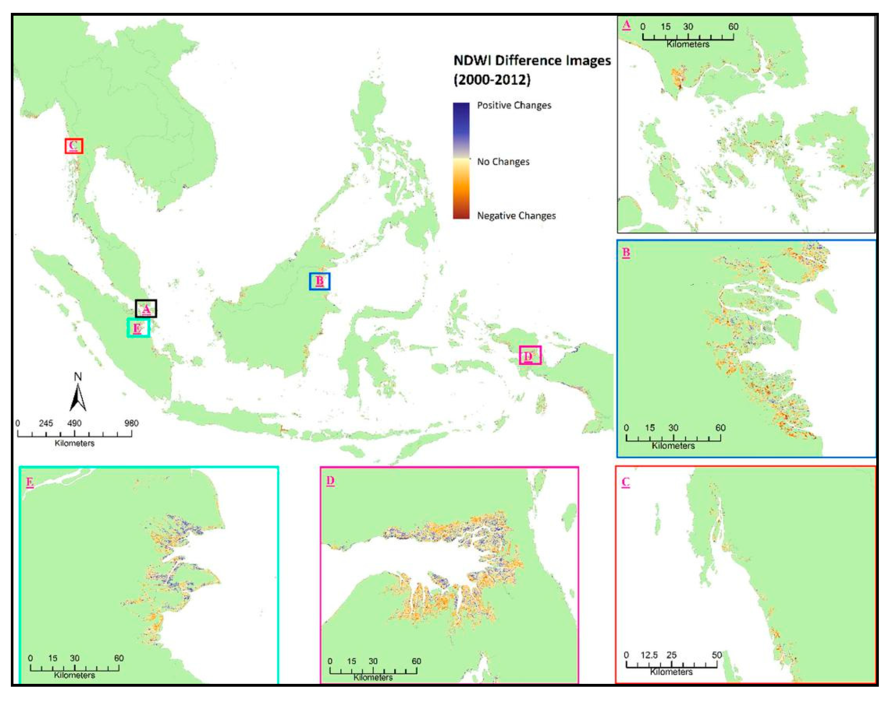
3.1. Spatiotemporal of MODIS Vegetation Indices in Mangrove Area

Figure 3 displays the NDVI difference images between 2000 and 2012. To achieve the most accurate visualization of changes, the largest deforested areas that corresponded to the land cover change drivers were selected. For urban conversion, the highlighted areas included Malaysia and Singapore. North Kalimantan corresponds to aquaculture conversion, Thailand corresponds to rice field conversion, South Sumatra corresponds to conversion to oil palm plantations, and mangrove regrowth was found in Papua. Positive changes imply that the index value in 2000 increased, while negative changes imply that the index value in 2000 decreased. The NDVI difference images provided more insight into the drivers of mangrove deforestation. It can be clearly observed that the vegetation index had different responses depending on the different drivers. In (A) Malaysia–Singapore and (B) North Kalimantan, the figure shows a slight decrease in vegetation in the mangrove sites. In (C) Thailand, the figure shows a smaller decrease in vegetation. In (E) South Sumatra, the figure shows an increase in NDVI. In (D) Papua, the NDVI increased in some areas, but most demonstrated no signs of change. In terms of healthiness, no change in NDVI implies no vegetation damage, as the density of vegetation is the same, indicating that there was no deforestation from 2000 to 2012.

The NDWI difference images provide more insight into the mangrove moisture condition. A decrease in the NDWI implies that the water content of mangroves is decreasing [109]. Figure 4 displays the NDWI difference between 2000 and 2012 with the highlighted areas representing the NDVI difference images. It can be clearly observed that the water index had a different response to each driver. In (A) Malaysia–Singapore and (B) North Kalimantan, which were deforested for urban and aquaculture conversion, respectively, the figure shows a slight decrease in water content for the mangrove sites. In (C) Thailand, the NDWI shows a smaller decrease. In (E) South Sumatra, there was an increase in the NDWI. This trend is also displayed in (D) Papua, where the NDWI increased in some areas, but overall, there was no relative change. As mangroves are considered an evergreen vegetation, a higher or decreasing NDWI indicates that the mangrove’s condition is damaged.

The SAVI difference images provide more insight into the canopy height of the mangrove forests. The higher the SAVI value, the higher the vegetation canopy [108]. In Figure 5, it can be clearly observed that the SAVI has different responses to each driver. In (A) Malaysia–Singapore and (B) North Kalimantan, the figure shows a severe decrease in canopy height. In (C) Thailand, there was deforestation due to rice plantations; hence, the figure shows a lower decrease in canopy height. In (E) South Sumatra, there was deforestation due to oil palm plantations, and the figure shows an increase in SAVI. The same trend was observed in (D) Papua, where the SAVI increased for some areas but most had no signs of change. From these results, the SAVI could be a potential index for detecting oil palm expansion over mangrove area, as reported by previous research [118]. However, it could be misinterpreted if no other information is available.

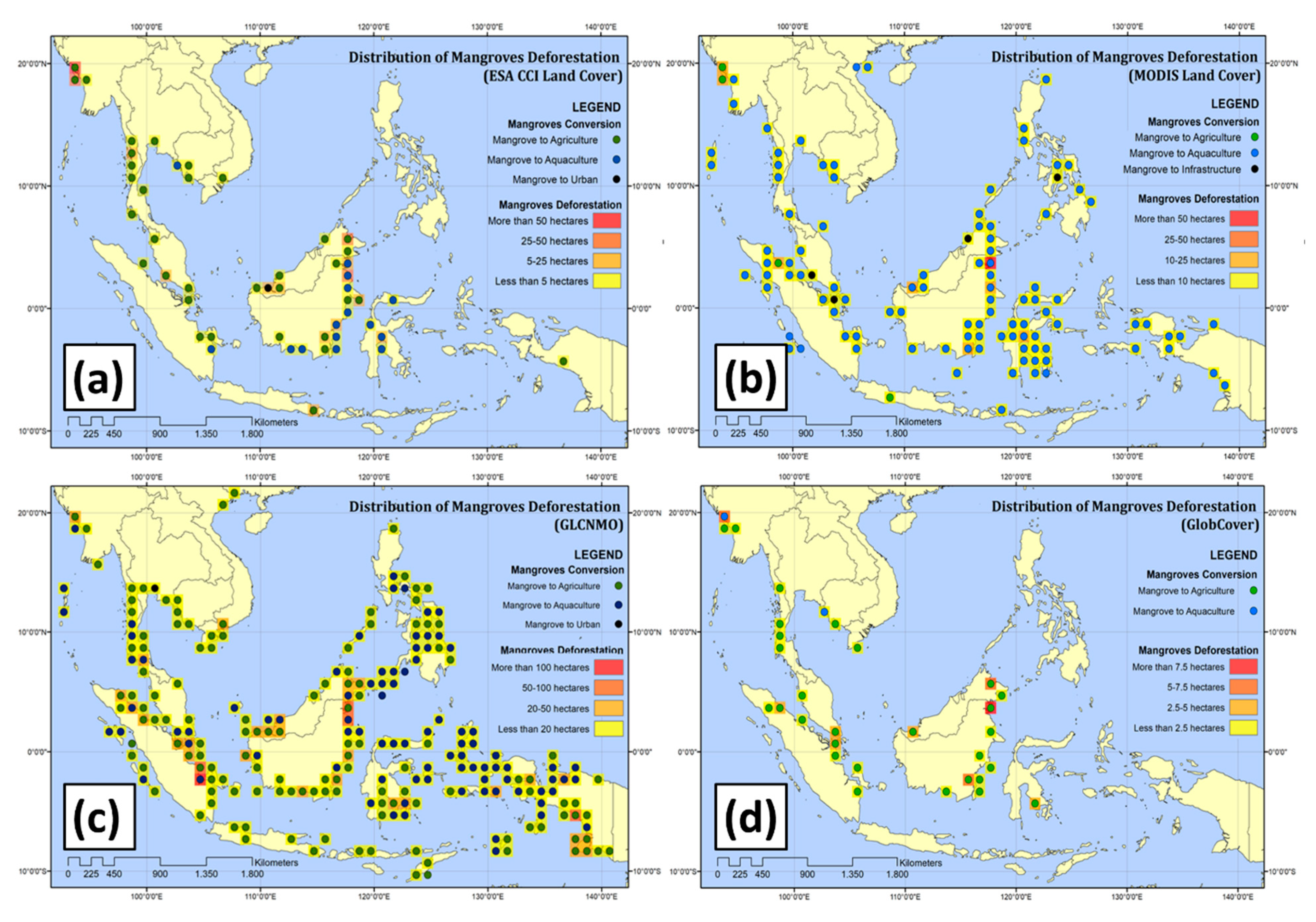
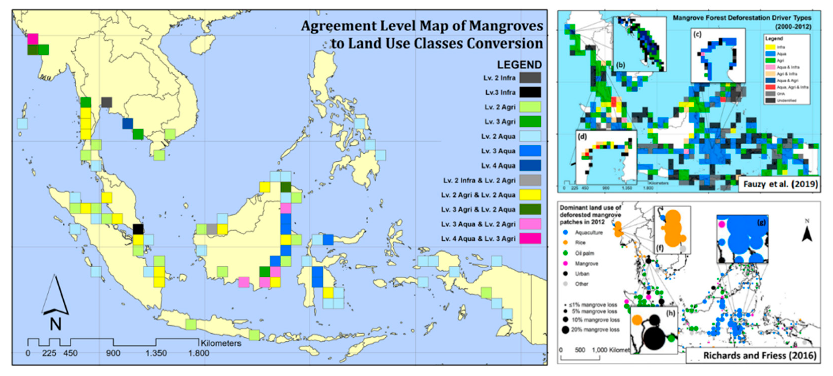
3.2. Results of Land Cover Conversion from Deforested Mangroves in Southeast Asia

From the ESA CCI Land Cover product, Figure 6a shows that the rate of deforestation in Myanmar is large, where, averaged over one grid, more than 50 ha of mangroves were converted into the farming class. This was followed by Indonesia, where fishery and farming in Kalimantan and Sulawesi are the major contributors to mangrove deforestation, with the average over one grid cell being 5–25 ha. The product of MODIS Land Cover (Figure 6b) shows that Indonesia has the highest amount of mangrove deforestation owing to the fishery class that has spread across Sumatra, Kalimantan, Sulawesi, and Papua, averaging at 10–25 ha of deforested mangrove. Myanmar also has a high deforestation level; approximately 25–50 ha of deforested mangroves averaged over one grid cell were converted to the farming and fishery classes. From the GLCNMO results, Figure 6c shows that Indonesia has the highest number of deforestation points due to the spread of the farming classes from Sumatra to Papua, with an average deforested area of 50–100 ha. Meanwhile, Malaysia and the Philippines have mangrove deforestation points due to changes in land cover, with an average of less than 50 ha. As observed from the GlobCover product results (Figure 6d), Indonesia has the highest deforestation point distribution as a consequence of the farming class spreading across Sumatra and Kalimantan, with an average deforestation of less than 10 ha. Myanmar has a significant deforestation point where one point of mangrove deforestation of more than 7.5 ha has been converted into the farming class.

Figure 7 is a map displaying the confidence levels in mangrove forest conversion obtained by combining all GLC products with the same land cover conversion classes from mangrove forests (farming, fishery, and housing) within a 1° grid cell. The confidence level is ranked from lowest to highest; level 1 means that the land cover conversion class is recognized by one GLC product, while level 4 means that the land cover conversion class in that location is recognized by all GLC products. This agreement level map (Figure 7) does not show the accuracy of each GLC product while detecting deforestation classes or the mangrove land cover changes. However, the confidence level illustrates the occurrence of spatial conversion from mangrove forests to land cover classes, as recognized by the GLC products in this study. Figure 7 shows that the highest confidence levels are in degraded mangrove areas, i.e., in Myanmar caused by farming, Indonesia caused by fisheries, and Malaysia caused by housing.

3.3. Mangrove Coefficient Growth

The value of Kc in each country in Southeast Asia ranges from 0.01 to approximately 1.3. This value indicates the growth rate of mangroves; a value close to 0 implies that the mangrove is not growing, and a value close to 1.3 implies the opposite. Some mangrove forests in Southeast Asia follow the dry rainy seasons, whereas others do not. The dry season usually occurs from April to September, and the rainy season from October to March. As shown in Figure 8, the countries that follow the seasonal pattern are Cambodia, Myanmar, and Thailand; other countries, such as Indonesia, Brunei Darussalam, Malaysia, and the Philippines, do not follow this seasonal pattern.

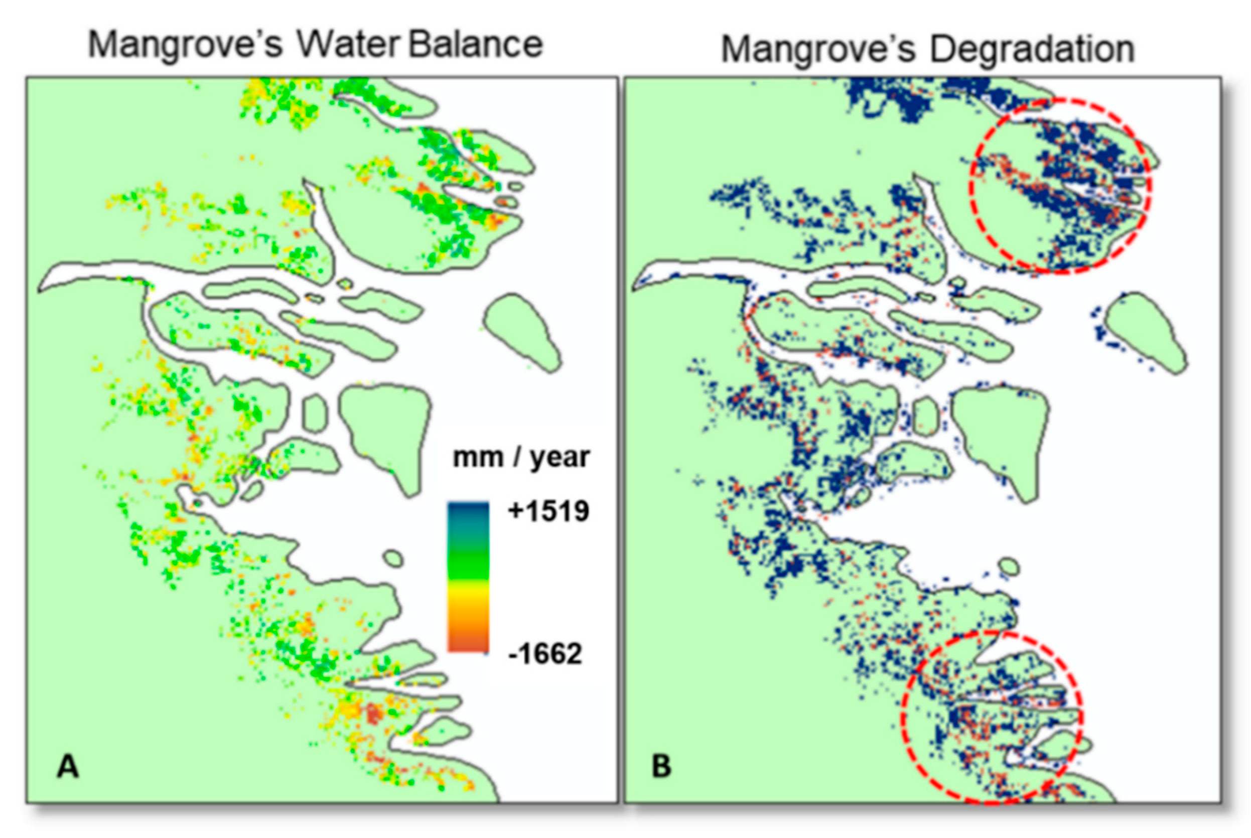
3.4. Mangrove Forests’ Water Balance for Degradation and Depletion Identification

The resulting values in the form of water balance deficits and surpluses are shown in Figure 9. In Cambodia, Myanmar, and Thailand, the values of deficit and surplus followed the pattern of dry and rainy seasons, respectively, while in Indonesia, Brunei Darussalam, Malaysia, and the Philippines, they did not follow the seasonal patterns.

As shown in Figure 10, this research shows that natural drivers have a larger effect on mangrove forests’ degradation and depletion compared with anthropogenic drivers. In this study, the determination of the effect of natural drivers focuses on evapotranspiration and precipitation data, as well as other meteorological phenomena such as whether or not regional patterns follow seasonal variation. The classification “mangroves at risk” refers to regions where the water balance is in deficit but not yet degraded. This should encourage policy makers to enforce the necessary steps to prevent mangrove degradation, recognizing the many advantages mangroves bring to society and the natural environment.

4. Discussion

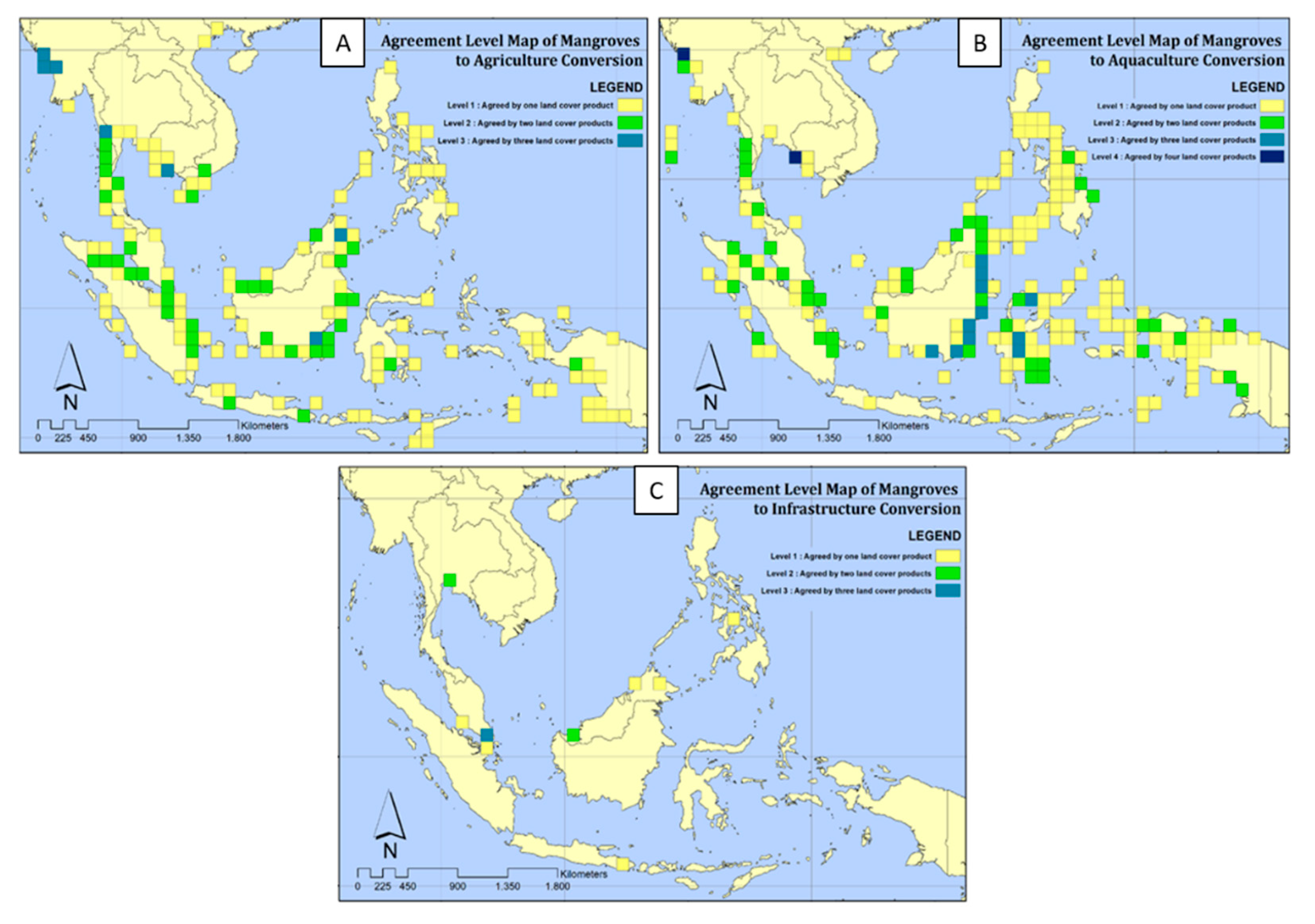
4.1. Mangrove Agreement Level

Agreement analysis is used to compare the similarity of various data with the same product level [119]. In this study, agreement analysis was used to compare four mangrove distribution datasets by making four levels of agreement. The first level indicates low agreement, level 2 indicates moderate agreement, level 3 indicates high agreement, and level 4 indicates very high agreement. Mangrove distribution data that will be compared are World Atlas of Mangroves v 1.1 for the period 1999–2003 [53], Global Distribution of Mangrove USGS v 1.3 for the period 1997–2000 [40], Indonesia Mangrove Map for the period 2006–2009 [54], and Global Mangrove Watch for the period 2010 [55]. Figure 11 shows that the majority of the level 4 mangrove agreements are in the Bintuny Bay (Papua) area. In the area of Sumatra, especially South Sumatra, the majority of mangrove agreements are level 3. Meanwhile, the majority of mangrove agreements for level 1 and 2 are on the island of Kalimantan.

Figure 12 shows the percentage level of agreement for each mangrove distribution. The USGS Global Distribution of Mangrove (v 1.3) has the highest percentage agreement among other products at level 4 (47%), while level 3, level 2 and level 1 have a percentage of 31%, 13%, and 9%, respectively. The mangrove distribution dataset that has the second highest value at level 4 is Global Mangrove Watch at 45%, while level 3, level 2 and level 1 are 33%, 14%, and 8%, respectively. World Atlas of Mangroves has a value of 43% for level 4, 16% for level 3, 14% for level 2, and 27% for level 1, while Indonesia Mangrove Map has a value of 25% for level 4, 21% for level 3, 16% for level 2, and 38% for level 1. It can be seen that the USGS Global Distribution of Mangroves (v 1.3) has the highest agreement value, so this study uses the USGS Global Distribution of Mangroves (v 1.3) as the distribution of mangroves.

4.2. Conformity of Data Products with DLUDMP and SEAMCT

The consistency of each land cover product was evaluated with reference to DLUDMP [10] and SEAMCT [52] in terms of the rate and the trigger of mangrove deforestation in Southeast Asia from 2000 to 2012. For this purpose, research related to the function of the dominant land in deforested mangrove areas from 2001 to 2012 as well as Southeast Asian mangrove conversion types were used for comparative data to assess the accuracy of the land cover conversion results obtained from each product of GLC. The calculation of the percentage of data products existing in one single land cover class was carried out in a 1° × 1° grid.

In the spatial context, this study illustrates that the points of mangrove forest conversion are similar to those in DLUDMP and SEAMCT. Figure 13 shows the locations of mangrove forest conversion, which is recognized by three to four GLC products, as mentioned previously. The results show that the conversion of mangrove forests into the farming class mostly occurred in the Rakhine region, Myanmar. The Myanmar government has strong policies that support national food security through increased rice production. As a result, many mangrove forests have been converted into paddy fields [120]. The conversion of mangrove forests into the fishery class mostly occurred in East Kalimantan and Sulawesi, Indonesia. The expansion of fisheries was driven by Indonesia’s government policies, which were aimed at making the country the largest fish producer in the world by 2015 [121]. Meanwhile, mangrove forests were converted to land for the housing class in the peninsulas of Malaysia and Singapore.

To the best of our knowledge, this research is the first to compare GLC products for monitoring mangrove deforestation over large areas. The approach used in this study is accompanied by certain assumptions to make the comparison of each GLC product easier (owing to the fact that these products have different characteristics). These assumptions, therefore, limit the quantitative comparison among different GLC products and increase the potential for bias in the results. In addition, the results cannot represent an assessment of the overall quality of each GLC product. However, the study focuses on drawing conclusions and finding policy recommendations for monitoring mangrove deforestation.

In general, based on the areas of mangrove forests converted into other land cover classes as shown in

Table 7. Conformity percentage between each data product with DLUDMP land use classes and SEAMCT based on the area of deforested mangrove.

Mangrove Forest Conversion Area Based on Global Land Cover Data Products (GLCM)		Width Percentage (GLCM)	Width Percentage (DLUDMP)	Width Percentage (SEAMCT)	Difference between GLCM and DLUDMP	Difference between GLCM and SEAMCT
MODIS (2001 dan 2012)	Farming	8.19%	52.70%	77.59%	44.52%	69.40%
	Fishery	88.12%	41.47%	20.05%	46.65%	68.08%
	Housing	3.69%	5.83%	2.36%	2.14%	1.33%
GlobCover (2005 and 2009)	Farming	92.42%	52.70%	77.59%	39.71%	14.83%
	Fishery	5.76%	41.47%	20.05%	35.71%	14.29%
	Housing	1.83%	5.83%	2.36%	4.00%	0.54%
ESA CCI LC (2001 and 2012)	Farming	77.07%	52.70%	77.59%	24.36%	0.52%
	Fishery	21.85%	41.47%	20.05%	19.62%	1.81%
	Housing	1.08%	5.83%	2.36%	4.75%	1.29%
GLCNMO (2008 and 2012)	Farming	55.63%	52.70%	77.59%	2.92%	21.96%
	Fishery	44.26%	41.47%	20.05%	2.79%	24.21%
	Housing	0.12%	5.83%	2.36%	5.71%	2.25%

, the similarity of each GLC product to DLUDMP-SEAMCT varies by different proportions, from 40% to 60% to less than 2%. Among the global land cover products, GLCNMO shows the highest conformity to DLUDMP, with an average difference of 3.81%. ESA CCI LC has the highest conformity to SEAMCT, with a mean difference of approximately 1.21%.

4.3. Uncertainties in Mangrove Change Data

As shown in Figure 14, the number of pixels located in the mangrove pixel class produced by MODIS Land Cover (2001 and 2012) reaches 4000 km², with 1000 km² of deforestation. In ESA CCI LC (2001 and 2012), the total area of the mangrove forest class reached 37,500 km², with a deforested area of 6500 km². In GlobCover (2005 and 2009), the total mangrove forest reached 28,000 km² and showed no signs of significant deforestation. Lastly, the area of mangrove forest class produced by GLCNMO (2008 and 2012) from the global land cover products was very similar to the area of mangrove owned by CGMFC-21. Hence, the assumptions made for the harmonization of the mangrove forest classes can be considered correct. Furthermore, the area of the mangrove forest measured by all products of GLC declined for several years, indicating widespread mangrove deforestation in that time period. The variations in the total area of mangrove forest could be caused by different methods of data acquisition, classification techniques, class definitions, and the production year of each land cover product.

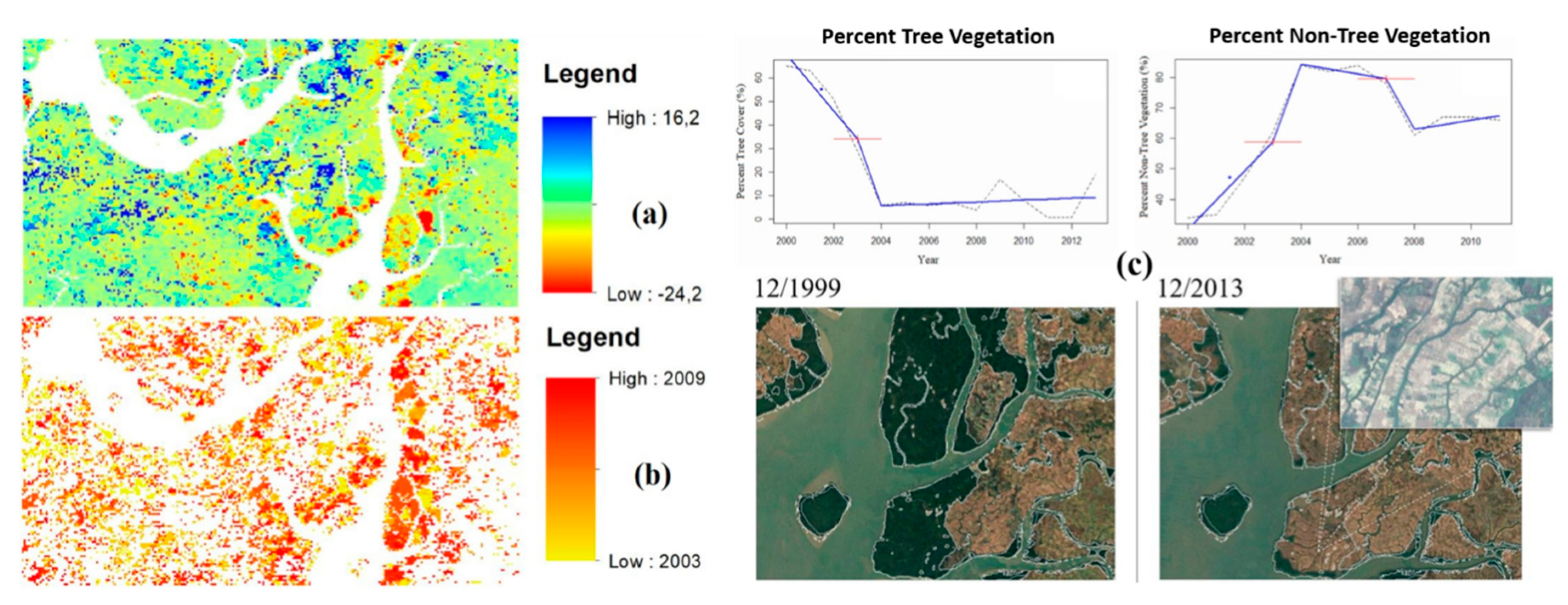
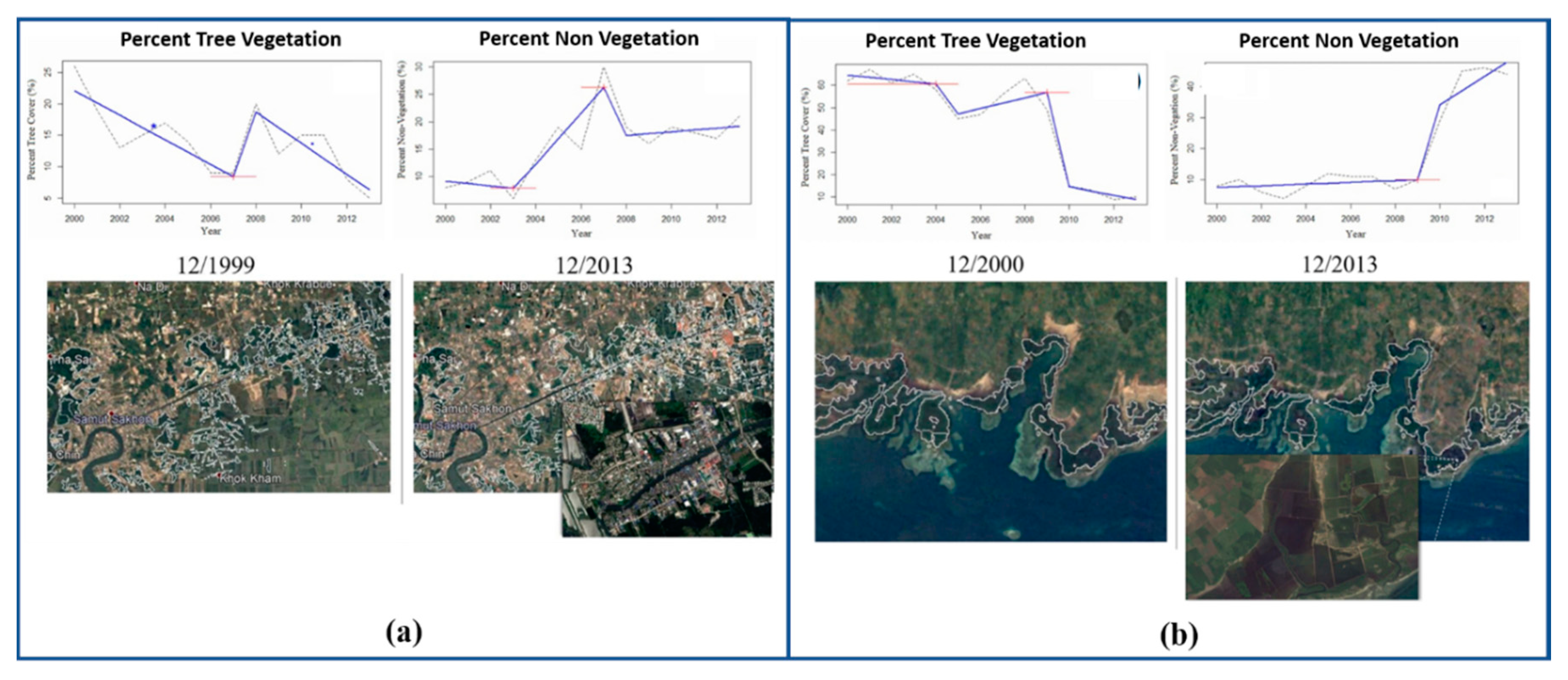
4.4. Trend Analysis and Breakpoint Detection on Deforested and Degraded Mangrove Area

PTC, PNTV, and PNV data were applied to identify extreme deforestation events (e.g., agriculture expansion in Myanmar, infrastructure expansion in Thailand, and aquaculture expansion in Indonesia) using trend analysis and breakpoint detection as explained below. Figure 15 shows a sample of a mangrove deforestation area driven by agriculture expansion in Rakhine State, Myanmar, as explained in the PTC trend. Positive values indicate an increase in PTC, while negative values indicate a decrease.

We detected 1269 grids with a 250 m spatial resolution that show the area converted for agriculture use in Rakhine State, Myanmar. Using trend analysis, at least 911 or 71.79% of those grids showed there was a negative trend in PTC and a positive trend in PNTV from 2000 to 2013. Using breakpoint detection in a particular grid, we revealed that the expansion occurred in 2003 when the PTC dropped and the PNTV jumped (Figure 15c). In Myanmar, especially in Rakhine State, nearly 70% of mangrove forests have been degraded since 1983 due to the vast expansion of rice farming as a consequence of the low productivity levels and competition [122,123].

Figure 16a portrays infrastructure expansion in Samut Sakhon State, Thailand. Trend analysis of PTC and PNV data indicated that 18 out of the 21 grids (75%) showed a negative trend in PTC and a positive trend in PNV. Meanwhile, the breakpoint detection discovered that the expansion happened in 2007, when the PTC dropped and PNV jumped in the same year (Figure 16a). According to the earlier studies, mangrove forests around the coastal areas of the Thailand Peninsula, which has a dense urban population, e.g., Phuket, Songkhla, and Phang Nga, were converted to residential areas and tourism facilities [124].

In Northern Sulawesi, Indonesia, trend analysis of PTC and PNV data revealed that 291 out of 309 grids (94.14%) showed a negative trend in PTC and positive trend in PNV. Meanwhile, the breakpoint detection identified that most of the mangrove forest conversion in this region occurred in 2009 (Figure 16b). As reported in previous research, the very rapid decline of mangrove forest in this area was due to major brackish-water pond developments [121].

4.5. Future Possible Directions

To detect other drivers of mangrove deforestation, other satellite-derived indices should be studied. For more information on the indices, higher spatial resolution datasets, such as Landsat and Sentinel, are needed to better establish their utility beyond the initial findings of this study. Implementing trend analysis and a break point detection algorithm to NDVI, NDWI, and SAVI for a time series analysis could form the basis of future studies. Another potential direction is a deeper phenology analysis based on water balance and remote sensing indices using long-term data. The continuous use of remote sensing indices will help to detect spatial and temporal changes in mangrove deforestation; thus, necessary steps toward mitigation can be planned and regulated.

The addition of other anthropogenic and naturogenic factors is crucial to the validation and completion of this research. Moreover, the spatial resolution used in this study should be improved and synchronized to increase the minimum level of detail and make it easily comparable. Notably, the approach used in this study can be used as an alternative for conducting a spatiotemporal analysis of a phenomenon on a regional or global scale. In addition, the method used in the consistency test stage can also be adopted to test the accuracy of information on various remote sensing data products involving similar topics. The combination of all available multi-temporal GLC products with a robust methodology for investigating global forest change would be the next stage of this research. Although this study has revealed that mangroves have been converted for various land uses, mangrove rehabilitation is still being conducted. Many concerned players have already made collaborative efforts in designing pilot projects for mangrove protection. Rehabilitation activities are abundant in Southeast Asian countries [125]; however, these have been deployed in relatively small areas, and the results are not noticeable because of the coarse spatial resolution of the data products. This research could be useful for designing mangrove forest rehabilitation strategies by combining the results of this study with supporting data [125].

Future applications that address environmental and socio-economic implications arising from these findings could be explored. The impact of this mangrove forest change on the environment, including on climate change [126], biodiversity [127], sea level rise, and coastal economies [128], could also be explored. Further investigations are required to elucidate the reason for this degradation change, such as the impact of long-term anthropogenic factors, that include cropland expansion and intensification change [129], urban change models [130], and water surface change [131] would enhance our ability to measure and improve future mangrove forest management [132,133].

5. Conclusions

The summary presented herein offers the primary points that will serve as the basis of future investigations. First, the relationships between remote sensing indices and deforestation drivers highly depend on the type of drivers. In future studies, exploring more satellite-derived indices could allow us to expose more deforestation drivers. Second, by adopting a trend analysis and break point detection in three difference sites, Rakhine State, Samut Sakhon, and North Sulawesi, we confirmed that mangrove forests were converted for agriculture, infrastructure, and aquaculture in 2003, 2007, and 2009, respectively. Moreover, the aggregation of PTV, PNV, and PNTV datasets is a highly recommended method of measuring the rate of changes, examining the degradation drivers, and tracing the exact year of expansion. Thirdly, the assimilation of GLC products revealed that agricultural and fishery classes are the predominant drivers in Southeast Asia, notably from 2001 to 2012. Although the study could not accurately describe the amount of mangrove conversion, the data processing and accuracy assessment method can be applied as an alternative method for conducting spatiotemporal analysis of either regional or global scale studies. Fourth, by analyzing the connection between the water balance and degradation of mangrove forests, we discovered that the natural drivers have a greater effect than the anthropogenic drivers. This finding could be investigated further by increasing the number of natural driver variables in the same spatial resolution, making the output more robust and comparable with the data of anthropogenic drivers. We hope that longer-term studies will be undertaken to determine how the water balance in Southeast Asian mangrove forests affect their level of degradation and depletion. Fifth, this extensive investigation leads us to deduce that we cannot easily determine a single factor as a sole driver of degradation in a particular mangrove patch. The combination of both anthropogenic and naturogenic drivers greatly affects and perhaps accelerates mangrove degradation. Finally, the abundance of remote sensing data and products recorded from extraterrestrial sensors could reveal valuable information required to understand and protect our terrestrial ecosystem, and it could be the foundation of important recommendations for creating impactful policy making.

References

1. Tomlinson, P.B. The Botany of Mangroves; Cambridge University Press: New York, NY, USA, 1986; ISBN 0-521-25567-8. [Google Scholar]
2. Alongi, D.M. Introduction in the Energetics of Mangrove Forests; Springer Science and Business Media BV: New York, NY, USA, 2009; pp. 47–64. [Google Scholar]
3. Kathiresan, K.; Bingham, B.L. Biology of mangroves and mangrove ecosystems. Adv. Mar. Biol. 2001, 40, 81–251. [Google Scholar] [CrossRef]
4. Brown, D. Mangrove: Nature’s Defences against Tsunamis; Environmental Justice Foundation: London, UK, 2004; ISBN 1-904523-05-7. [Google Scholar]
5. Feller, I.C.; Sitnik, M. Mangrove Ecology Workshop Manual; Smithsonian Institution: Washington, DC, USA, 1996. [Google Scholar]
6. Kirui, B.; Kairo, J.G.; Karachi, M. Allometric Equations for Estimating Above Ground Biomass of Rhizophora Mangroves at Gazi Bay, Kenya. West. Indian Ocean J. Mar. Sci. 2006, 5, 27–34. [Google Scholar] [CrossRef] [Green Version]
7. Spalding, M.; Blasco, F.; Field, C. World Atlas of Mangroves; Routledge: London, UK, 1997; p. 336. [Google Scholar]
8. Giesen, W. Indonesian mangroves part I: Plant diversity and vegetation. Trop. Biodivers. 1998, 5, 99–111. [Google Scholar]
9. Hamilton, S.E.; Casey, D. Creation of a high spatio-temporal resolution global database of continuous mangrove forest cover for the 21st century (CGMFC-21). Glob. Ecol. Biogeogr. 2016, 25, 729–738. [Google Scholar] [CrossRef]
10. Richards, D.R.; Friess, D.A. Rates and drivers of mangrove deforestation in Southeast Asia, 2000–2012. Proc. Natl. Acad. Sci. USA 2016, 113, 344–349. [Google Scholar] [CrossRef] [PubMed] [Green Version]
11. Fauzi., A.I.; Sakti, A.D.; Yayusman, L.F.; Harto, A.B.; Prasetyo, L.B.; Irawan, B.; Wikantika, K. Evaluating Mangrove Forest Deforestation Causes in Southeast Asia by Analyzing Recent Environment and Socio-Economic Data Products. In Proceedings of the 39th Asian Conference on Remote Sensing, Kuala Lumpur, Malaysia, 15–19 October 2018; pp. 880–889. [Google Scholar]
12. Foti, R.; Jesus, M.; Rinaldo, A.; Rodriguez-Iturbe, I. Signs of Critical Transition in The Everglades Wetlands in Response to Climate and Anthropogenic Changes. Proc. Natl. Acad. Sci. USA 2013, 10, 6296–6300. [Google Scholar] [CrossRef] [Green Version]
13. FAO. The World’s Mangroves 1980–2005; Forestry Paper FAO 153; FAO: Rome, Italy, 2007. [Google Scholar]
14. Woodroffe, C.D. The Impact of Sea-Level Rise on Mangrove Shorelines. Prog. Phys. Geogr. Earth Environ. 1990, 14, 483–520. [Google Scholar] [CrossRef]
15. Thomas, N.; Lucas, R.; Bunting, P.; Hardy, A.; Rosenqvist, A.; Simard, M. Distribution and drivers of global mangrove forest change 1996–2010. PLoS ONE 2017, 12, e0179302. [Google Scholar] [CrossRef] [Green Version]
16. Rioja-Nieto, R.; Barrera-Falcón, E.; Torres-Irineo, E.; Mendoza-González, G.; Cuervo-Robayo, A.P. Environmental drivers of decadal change of a mangrove forest in the North coast of the Yucatan peninsula, Mexico. J. Coast Conserv. 2017, 21, 167–175. [Google Scholar] [CrossRef]
17. Songsom, V.; Koedsin, W.; Ritchie, R.J.; Huete, A. Mangrove Phenology and Environmental Drivers Derived from Remote Sensing in Southern Thailand. Remote Sens. 2019, 11, 955. [Google Scholar] [CrossRef] [Green Version]
18. Valiela, I.; Bowen, J.; York, J. Mangrove Forests: One of The World’s Threatened Major Tropical Environments. Bioscience 2001, 51, 807–815. [Google Scholar] [CrossRef] [Green Version]
19. Cahoon, D.R.; Hensel, P.F.; Spencer, T.; Reed, D.J.; McKee, K.L.; Saintilan, N. Coastal Wetland Vulnerability to Relative Sea-Level Rise: Wetland Elevation Trends and Process Controls. In Wetlands and Natural Resource Management; Varhoeven, J.T.A., Beltman, B., Bobbink, R., Whigham, D.F., Eds.; Springer: Berlin/Heidelberg, Germany, 2006; Volume 190, pp. 271–292. ISBN 978-3-540-33187-2. [Google Scholar] [CrossRef]
20. MacKay, F.; Cyrus, D.; Russell, K.L. Macrobenthic invertebrate responses to prolonged drought in South Africa’s largest estuarine lake complex. Estuar. Coast. Shelf S. 2010, 86, 553–567. [Google Scholar] [CrossRef]
21. Bhat, N.R.; Suleiman, M.K. Classification of soils supporting mangrove plantation in Kuwait. Arch. Agron. Soil Sci. 2004, 50, 535–551. [Google Scholar] [CrossRef]
22. Almulla, L. Soil site suitability evaluation for mangrove plantation in Kuwait. World Appl. Sci. J. 2013, 22, 1644–1651. [Google Scholar]
23. Nusantara, M.A.; Hutomo, M.; Purnama, H. Evaluation and planning of mangrove restoration programs in Sedari Village of Kerawang District, West Java: Contribution of PHE-ONWJ coastal development programs. Procedia Environ. Sci. 2015, 23, 207–214. [Google Scholar] [CrossRef] [Green Version]
24. Boto, K.G.; Wellington, J.T. Soil characteristics and nutrient status in a Nothern Australian mangrove forest. Estuaries 1984, 7, 61–69. [Google Scholar] [CrossRef]
25. Chimner, R.A. Soil respiration rates of tropical peatlands in Micronesia and Hawaii. Wetlands 2004, 24, 51–56. [Google Scholar] [CrossRef]
26. Crain, C.M.; Silliman, B.R.; Bertness, S.L.; Bertness, M.D. Physical and biotic drivers of plaant distribution across estuarine salinity gradients. Ecology 2004, 85, 2539–2549. [Google Scholar] [CrossRef] [Green Version]
27. Ribeiro, J.P.N.; Tiberio, F.C.S.; de Oliveira, A.A. The role of soil nutrients in boundaries between mangrove and herbaceous assemblages in a tropical estuary. Biotropica 2015, 47, 517–520. [Google Scholar] [CrossRef]
28. Clarke, L.D.; Hannon, N.J. The mangrove swamp and salt marsh communities of the Sydney District: II. the holocoenotic complex with particular reference to physiography. J. Ecol. 1969, 57, 213–234. [Google Scholar] [CrossRef]
29. Primavera, J.H.; Savaris, J.D.; Bajoyo, B.; Coching, J.D.; Curnick, D.J.; Golbeque, R.; Guzman, A.T.; Henderin, J.Q.; Joven, R.V.; Loma, R.A.; et al. Manual on Community-Based Mangrove Rehabilitation - Mangrove Manual Series No.1; Zoological Society of London: London, UK, 2012; 240p, ISBN 978-971-95370-1-4. [Google Scholar]
30. Cohen, M.C.L.; Lara, R.J.; Cuevas, E.; Oliveras, E.M.; Sternberg, L.D.S. Effects of sea-level rise and climatic changes on mangroves from southwestern littoral of Puerto Rico during the middle and late holocene. Catena 2016, 143, 187–200. [Google Scholar] [CrossRef] [Green Version]
31. Asbridge, E.F.; Bartolo, R.; Finlayson, C.M.; Lucas, R.M.; Rogers, K.; Woodroffe, C.D. Assessing the distribution and drivers of maangrove dieback in Kakadu National Paark, nothern Australia. Estuar. Coast. Shelf Sci. 2019, 228, 1–12. [Google Scholar] [CrossRef]
32. Gupta, K.; Mukhopadhyay, A.; Giri, S.; Chanda, A.; Majumdar, S.D.; Samanta, S.; Mitra, D.; Samal, R.N.; Pattnaik, A.K.; Hazra, S. An index for discrimination of mangroves from non-mangroves using LANDSAT 8 OLI imagery. MethodsX 2018, 5, 1129–1139. [Google Scholar] [CrossRef] [PubMed]
33. Ahmed, K.R.; Akter, S. Analysis of landcover change in southwest Bengal delta due to floods by NDVI, NDWI and K-means cluster with landsat multi-spectral surface reflectance satellite data. Remote Sens. Appl. Soc. Environ. 2017, 8, 168–181. [Google Scholar] [CrossRef]
34. Pastor-Guzman, J.; Dash, J.; Atkinson, P.M. Remote sensing of mangrove forest phenology and its environmental drivers. Remote Sens. Environ. 2018, 205, 71–84. [Google Scholar] [CrossRef] [Green Version]
35. Yu, L.; Wang, J.; Li, X.; Li, C.; Zhao, Y.; Gong, P. A multi-resolution global land cover dataset through multisource data aggregation. Sci. China Earth Sci. 2014, 57, 2317–2329. [Google Scholar] [CrossRef]
36. Hailu, B.T.; Fekadu, M.; Nauss, T. Availability of global and national scale land cover products and their accuracy in mountainous areas of Ethiopia: A review. J. Appl. Remote Sens. 2018, 12, 041502. [Google Scholar] [CrossRef]
37. Pendrill, F.; Persson, U.M. Combining global land cover datasets to quantify agricultural expansion into forests in Latin America: Limitations and challenges. PLoS ONE 2017, 12, e0181202. [Google Scholar] [CrossRef]
38. Pérez-Hoyos, A.; Rembold, F.; Kerdiles, H.; Gallego, J. Comparison of Global Land Cover Datasets for Cropland Monitoring. Remote Sens. 2017, 9, 1118. [Google Scholar] [CrossRef] [Green Version]
39. Tsendbazar, N.; Bruin, S.D.; Herold, M. Integrating global land cover datasets for deriving user-specific maps. Int. J. Digit. Earth 2017, 10, 219–237. [Google Scholar] [CrossRef] [Green Version]
40. Giri, C.; Ochieng, E.; Tieszen, L.L.; Zhu, Z.; Singh, A.; Loveland, T.; Duke, N. Status and distribution of mangrove forests of the world using earth observation satellite data. Glob. Ecol. Biogeogr. 2011, 20, 154–159. [Google Scholar] [CrossRef]
41. Hansen, M.C. High-Resolution Global Maps of 21st-Century Forest Cover Change. Science 2013, 342, 850–853. [Google Scholar] [CrossRef] [PubMed] [Green Version]
42. Coumou, D.; Rahmstorf, S. A decade of seather extremes. Nat. Clim. Chang. 2012, 2, 491–496. [Google Scholar] [CrossRef]
43. Bathiany, S.; Dakos, V.; Scheffer, M.; Lenton, T.M. Climate models predict increasing temperaature variability in poor countries. Sci. Adv. 2018, 4, 1–10. [Google Scholar] [CrossRef] [Green Version]
44. Arnell, N.W. Climate change and global water resources: SRES emissions and socio-economic scenarios. Glob. Environ. Chang. 2004, 14, 31–51. [Google Scholar] [CrossRef]
45. Maslin, M.; Austin, P. Climate models at their limit? Nature 2012, 486, 183–184. [Google Scholar] [CrossRef] [PubMed]
46. Myhre, G.; Alterskjaer, K.; Stjern, C.W.; Hodnebrog, Ø.; Marelle, L.; Samset, B.H.; Sillmann, J.; Schaller, N.; Fischer, E.; Schulz, M.; et al. Frequency of extreme precipitation increases extensively with event rareness under global warming. Sci. Rep. 2019, 9, 16063. [Google Scholar] [CrossRef] [PubMed] [Green Version]
47. Fischer, E.M.; Knutti, R. Detection of spatially aggregated changes in temperature and precipitation extremes. Geophys. Res. Lett. 2014, 41, 547–554. [Google Scholar] [CrossRef]
48. Duke, N.C.; Kovacs, J.M.; Griffths, A.D.; Preece, L.; Hill, D.J.E.; Oosterzee, P.; Mackenzie, J.; Morning, H.S.; Burrows, D. Large-Scale Dieback of Mangroves in Australia’s Gulf of Carpentaria: A Severe Ecosystem Response, Coincidental with an Unusually Extreme Weather Event. Mar. Freshw. Res. 2017, 68, 1816–1829. [Google Scholar] [CrossRef]
49. Jones, R. Quantifying Extreme Weather Event Impacts on the Northern Gulf Coast Using Landsat Imagery. J. Coast. Res. 2015, 31, 1229–1240. [Google Scholar] [CrossRef]
50. Pettorelli, N. The Normalized Difference Vegetation Index; Oxford University Press: Oxford, UK, 2013; ISBN 978-0199693160. [Google Scholar]
51. Ibharim, N.A.; Mustapha, M.A.; Lihan, T.; Mazlan, A.G. Mapping Mangrove Changes in The Matang Mangrove Forest Using Multi Temporal Satellite Imageries. Ocean Coast. Manag. 2015, 114, 64–76. [Google Scholar] [CrossRef]
52. Fauzi, A.; Sakti, A.; Yayusman, L.; Harto, A.; Prasetyo, L.; Irawan, B.; Kamal, M.; Wikantika, K. Contextualizing Mangrove Forest Deforestation in Southeast Asia Using Environmental and Socio-Economic Data Products. Forests 2019, 10, 952. [Google Scholar] [CrossRef] [Green Version]
53. Spalding, M.; Kainuma, M.; Collins, L. World Atlas of Mangrove, Version 3.0; A collaborative project of ITTO, ISME, FAO, UNEP-WCMC, UNESCO-MAB, UNU-INWEH and TNC; Earthscan: London, UK, 2010; 319p. [Google Scholar]
54. Saputro, G.B.; Hartini, S.; Sukardjo, S.; Susanto, A.; Poniman, A. Peta Mangroves Indonesia; Bakosurtanal: Bogor, Indonesia, 2012. [Google Scholar]
55. Bunting, P.; Rosenqvist, A.; Lucas, R.M.; Rebelo, L.-M.; Hilarides, J.; Thomas, N.; Hardy, A.; Itoh, T.; Shimada, M.; Finlayson, C.M. The global mangrove watch–a new 2010 global baseline of mangrove extent. Remote Sens. 2018, 10, 1669. [Google Scholar] [CrossRef] [Green Version]
56. Olson, D.M.; Dinerstein, E.; Wikramanayake, E.D.; Burgess, N.D.; Powell, G.V.N.; Underwood, E.C.; D’amico, J.A.; Itoua, I.; Strand, H.E.; Morrison, J.C.; et al. Terrestrial Ecoregions of the World: A New Map of Life on Earth: A new global map of terrestrial ecoregions provides an innovative tool for conserving biodiversity. BioScience 2001, 51, 933–938. [Google Scholar] [CrossRef]
57. Friedl, M.; Sulla-Menashe, D. MCD12Q1 MODIS/Terra+Aqua Land Cover Type Yearly L3 Global 500m SIN Grid V006 [Data set]. NASA EOSDIS Land Process. DAAC 2015. [Google Scholar] [CrossRef]
58. Carroll, M.L.; DiMiceli, C.M.; Wooten, M.R.; Hubbard, A.B.; Sohlberg, R.A.; Townshend, J.R.G. MOD44W MODIS/Terra Land Water Mask Derived from MODIS and SRTM L3 Global 250m SIN Grid V006 [Data set]. NASA EOSDIS Land Process. DAAC 2017. [Google Scholar] [CrossRef]
59. Pesaresi, M.; Ehrlich, D.; Ferri, S.; Florczyk, A.J.; Freire, S.; Halkia, S.; Julea, A.M.; Kemper, T.; Soille, P.; Syrris, V. Operating Procedure for the Production of the Global Human Settlement Layer from Landsat Data of the Epochs 1975, 1990, 2000, and 2014; Publications Oce of the European Union EUR 27741 EN: Ispra, Italy, 2016. [Google Scholar] [CrossRef]
60. Goldewijk, K.K.; Beusen, A.; Doelman, J.; Stehfest, E. Anthropogenic land-use estimates for the Holocene—HYDE 3.2. Earth Syst. Sci. Data 2017, 9, 927–953. [Google Scholar] [CrossRef] [Green Version]
61. NGDC NOAA, Version 4 DMSP-OLS Nighttime Lights Time Series. Available online: https://ngdc.noaa.gov/eog/dmsp/downloadV4composites.html (accessed on 8 August 2019).
62. Kummu, M.; Taka, M.; Guillaume, J.H.A. Gridded global datasets for Gross Domestic Product and Human Development Index over 1990–2015. Sci. Data 2018, 5, 180004. [Google Scholar] [CrossRef] [Green Version]
63. Doxsey-Whitfield, E.; MacManus, K.; Adamo, S.B.; Pistolesi, L.; Squires, J.; Borkovska, O.; Baptista, S.R. Taking Advantage of the Improved Availability of Census Data: A First Look at the Gridded Population of the World, Version 4. Pap. Appl. Geogr. 2015, 1, 226–234. [Google Scholar] [CrossRef]
64. ESA-European Space Agency. Land Cover CCI Product User Guide, Version 2; ESA CCI LC Project; European Space Agency: Paris, France, 2017. [Google Scholar]
65. Friedl, M.A.; Menashe, D.S.; Tan, B.; Schneider, A.; Ramankutty, N.; Sibley, A.; Huang, X. MODIS Collection 5 global land cover: Algorithm refinements and characterization of new datasets. Remote. Sens. Environ. 2010, 114, 168–182. [Google Scholar] [CrossRef]
66. Bontemps, S.; Defourny, P.; Van Bogaert, E.; Arino, O.; Kalogirou, V.; Ramos Pérez, J. GlobCover 2009. Products Description and Validation Report. Available online: http://due.esrin.esa.int/files/GLOBCOVER2009_Validation_Report_2.2.pdf (accessed on 12 June 2019).
67. Bicheron, P.; Huc, M.; Henry, C.; Bontemps, S.; Lacaux, J.P. GlobCover Products Description Manual; European Space Agency: Paris, France, 2008; p. 25. [Google Scholar]
68. Tateishi, R.; Uriyangqai, B.; Al-Bilbisi, H.; Aboel Ghar, M.; Tsend-Ayush, J.; Kobayashi, T.; Kasimu, A.; Thanh Hoan, N.; Shalaby, A.; Alsaaideh, B.; et al. Production of global land cover data—GLCMO. Int. J. Digit. Earth 2011, 4, 22–49. [Google Scholar] [CrossRef]
69. Tateishi, R.; Hoan, N.; Kobayashi, T.; Alsaaideh, B.; Tana, G.; Pong, D. Production of Global Land Cover Data—GLCNMO2008. J. Geogr. Geol. 2014, 6, 99–122. [Google Scholar] [CrossRef] [Green Version]
70. Didan, K. MOD13Q1 MODIS/Terra Vegetation Indices 16-Day L3 Global 250 m SIN Grid V006 [Data set]. NASA EOSDIS Land Process. DAAC 2015. [Google Scholar] [CrossRef]
71. Didan, K. MOD13A1 MODIS/Terra Vegetation Indices 16-Day L3 Global 500m SIN Grid V006 [Data set]. NASA EOSDIS Land Process. DAAC 2015. [Google Scholar] [CrossRef]
72. Hu, T.; Su, Y.; Xue, B.; Liu, J.; Zhao, X.; Fang, J.; Guo, Q. Mapping Global Forest Aboveground Biomass with Spaceborne LiDAR, Optical Imagery, and Forest Inventory Data. Remote Sens. 2016, 8, 565. [Google Scholar] [CrossRef] [Green Version]
73. Mutanga, O.; Skidmore A., K. Narrow band vegetation indices overcome the saturation problem in biomass estimation. Int. J. Remote Sens. 2004, 25, 3999–4014. [Google Scholar] [CrossRef]
74. Spawn, S.A.; Sullivan, C.C.; Lark, T.J.; Gibbs, H.K. Harmonized global maps of above and belowground biomass carbon density in the year 2010. Sci. Data 2020, 7, 112. [Google Scholar] [CrossRef]
75. Running, S.; Mu, Q. MOD16A2 MODIS/Terra Evapotranspiration 8-day L4 Global 500m SIN Grid. NASA LP DAAC 2015. [Google Scholar] [CrossRef]
76. Funk, C.; Peterson, P.; Landsfeld, M.; Pedreros, D.; Verdin, J.; Shukla, S.; Husak, G.; Rowland, J.; Harrison, L.; Hoell, A.; et al. The climate hazards infrared precipitation with stations—A new environmental record for monitoring extremes. Sci. Data 2015, 2, 150066. [Google Scholar] [CrossRef] [Green Version]
77. Janowiak, J.E.; Joyce, R.J.; Yarosh, Y. A Real-Time Global Half-Hourly Pixel-Resolution Infrared Dataset and Its Applications. Bull. Amer. Meteor. Soc. 2001, 82, 205–218. [Google Scholar] [CrossRef] [Green Version]
78. Saha, S.; Moorthi, S.; Pan, H.; Wu, X.; Wang, J.; Nadiga, S.; Tripp, P.; Kistler, R.; Woollen, J.; Behringer, D.; et al. The NCEP Climate Forecast System Reanalysis. Bull. Amer. Meteor. Soc. 2010, 91, 1–146. [Google Scholar] [CrossRef]
79. Peterson, P.; Funk, C.C.; Landsfeld, M.F.; Husak, G.J.; Pedreros, D.H.; Verdin, J.P.; Rowland, J.; Shukla, S.; McNally, A.; Michaelsen, J.; et al. The Climate Hazards Group Infrared Precipitation with Stations (CHIRPS) Dataset: Quasi-Global Precipitation Estimates for Drought Monitoring and Trend Analysis. In Proceedings of the American Geophysical Union Fall Meeting, San Francisco, CA, USA, 15–19 December 2014. [Google Scholar]
80. Dimiceli, C.; Carroll, M.; Sohlberg, R.; Kim, D.H.; Kelly, M.; Townshend, J.R.G. MOD44B MODIS/Terra Vegetation Continuous Fields Yearly L3 Global 250m SIN Grid V006 [Data set]. NASA EOSDIS Land Process. DAAC 2015. [Google Scholar] [CrossRef]
81. Herold, M.; Schmullius, C. Report on the Harmonization of Global and Regional Land Cover Products Meeting; FAO: Rome, Italy, 2004; Available online: https://gofcgold.org/sites/default/files/docs/GOLD_20.pdf (accessed on 14 April 2020).
82. Herold, M.; Woodcock, C.; Gregorio, A.D.; Mayaux, P.; Latham, A.B.; Schmullius, C.C. A joint initiative for harmonization and validation of land cover datasets. IEEE Trans. Geosci. Remote Sens. 2006, 44, 1719–1727. [Google Scholar] [CrossRef]
83. Roy, S.; Mahapatra, M.; Chakraborty, A. Mapping and monitoring of mangrove along the Odisha coast based on remote sensing and GIS techniques. Model. Earth Syst. Environ. 2019, 5, 217–226. [Google Scholar] [CrossRef]
84. Rhyma, P.; Norizah, K.; Hamdan, O.; Faridah-Hanum, I.; Zulfa, A. Integration of normalised different vegetation index and Soil-Adjusted Vegetation Index for mangrove vegetation delineation. Remote Sens. Appl. 2020, 17, 100280. [Google Scholar] [CrossRef]
85. Verbesselt, J.; Hyndman, R.; Zeileis, A.; Culvenor, D. Phenological change detection while accounting for abrupt and gradual trends in satellite image time series. Remote Sens. Environ. 2010, 114, 2970–2980. [Google Scholar] [CrossRef] [Green Version]
86. Bai, J.; Perron, P. Computation and analysis of multiple structural change models. J. Appl. Econom. 2003, 18, 1–22. [Google Scholar] [CrossRef] [Green Version]
87. Forkel, M.; Carvalhais, N.; Verbesselt, J.; Mahecha, M.D.; Neigh, C.S.R.; Reichstein, M. Trend change detection in NDVI time series: Effects of inter-annual variability and methodology. Remote Sens. 2013, 5, 2113–2144. [Google Scholar] [CrossRef] [Green Version]
88. Reef, R.; Lovelock, C.E. Regulation of water balance in mangroves. Ann. Bot. 2015, 115, 385–395. [Google Scholar] [CrossRef] [Green Version]
89. Santini, N.S.; Reef, R.; Lockington, D.A.; Lovelock, C. The use of fresh and saline water sources by the mangrove Avicennia marina. Hydrobiologia 2015, 745, 59–68. [Google Scholar] [CrossRef]
90. Feng, M.; Bai, Y. A global land cover map produced through integrating multi-source datasets. Big Earth Data 2019, 3, 191–219. [Google Scholar] [CrossRef] [Green Version]
91. Jaafar, H.H.; Ahmad, F.A.; El Beyrouthy, N. GCN250, new global gridded curve numbers for hydrologic modeling and design. Sci. Data 2019, 6, 145. [Google Scholar] [CrossRef] [PubMed] [Green Version]
92. Buchhorn, M.; Lesiv, M.; Tsendbazar, N.-E.; Herold, M.; Bertels, L.; Smets, B. Copernicus Global Land Cover Layers—Collection 2. Remote Sens. 2020, 12, 1044. [Google Scholar] [CrossRef] [Green Version]
93. Lloyd, C.T.; Sorichetta, A.; Tatem, A.J. High resolution global gridded data for use in population studies. Sci. Data 2017, 4, 170001. [Google Scholar] [CrossRef] [Green Version]
94. Vancutsem, C.; Marinho, E.; Kayitakire, F.; See, L.; Fritz, S. Harmonizing and Combining Existing Land Cover/Land Use Datasets for Cropland Area Monitoring at the African Continental Scale. Remote Sens. 2013, 5, 19–41. [Google Scholar] [CrossRef] [Green Version]
95. Song, X.; Huang, C.; Townshend, J.R. Improving global land cover characterization through data fusion. Geo-Spat. Inf. Sci. 2017, 20, 141–150. [Google Scholar] [CrossRef] [Green Version]
96. Herold, M.; Mayaux, P.; Woodcock, C.E.; Baccini, A.; Schmullius, C. Some challenges in global land cover mapping: An assessment of agreement and accuracy in existing 1 km datasets. Remote Sens. Environ. 2008, 112, 2538–2556. [Google Scholar] [CrossRef]
97. Lu, M.; Wu, W.; Zhang, L.; Liao, A.; Peng, S.; Tang, H. A comparative analysis of five global cropland datasets in China. Sci. China Earth Sci. 2016, 59, 2307–2317. [Google Scholar] [CrossRef]
98. Fritz, S.; See, L.; Perger, C.; McCallum, I.; Schill, C.; Schepaschenko, D.; Duerauer, M.; Karner, M.; Dresel, C.; Laso-Bayas, J.-C.; et al. A global dataset of crowdsourced land cover and land use reference data. Sci. Data 2017, 4, 170075. [Google Scholar] [CrossRef] [Green Version]
99. Yang, Y.K.; Xiao, P.F.; Feng, X.Z.; Li, H.X. Accuracy assessment of seven global land cover datasets Journal Pre-proof Journal Pre-proof over China. ISPRS-J. Photogramm. Remote Sens. 2017, 125, 156–173. [Google Scholar] [CrossRef]
100. Islam, S.; Zhang, M.; Yang, H.; Ma, M. Assessing inconsistency in global land cover products and synthesis of studies on land use and land cover dynamics during 2001 to 2017 in the southeastern region of Bangladesh. J. Appl. Remote Sens. 2019, 13, 048501. [Google Scholar] [CrossRef]
101. Barnabe, G. Aquaculture; Ellis Horwood: New York, NY, USA, 1990; Volume I, ISBN 0-203-16883-6. [Google Scholar]
102. Webb, E.L.; Jachowski, N.R.A.; Phelps, J.; Friess, D.A.; Than, M.M.; Ziegler, A.D. Deforestation in the Ayeyarwady Delta and the conservation implications of an internationally-engaged Myanmar. Glob. Environ. Chang. 2014, 24, 321–333. [Google Scholar] [CrossRef]
103. Lai, S.; Loke, L.H.L.; Hilton, M.J.; Bouma, T.J.; Todd, P.A. The effects of urbanization on coastal habitats and the potential for ecological engineering: A Singapore case study. Ocean Coast. Manag. 2015, 103, 78–85. [Google Scholar] [CrossRef]
104. Weier, J.; Herring, D. Measuring Vegetation (NDVI & EVI); NASA Earth Observatory: Washington, DC, USA, 2000. Available online: https://earthobservatory.nasa.gov/features/MeasuringVegetation (accessed on 24 April 2020).
105. Cai, Z.; Jonsson, P.; Jin, H.; Eklundh, L. Performance of Smoothing Methods for Reconstructing NDVI Time-Series and Estimating Vegetation Phenology from MODIS Data. Remote Sens. 2017, 9, 1271. [Google Scholar] [CrossRef] [Green Version]
106. Meneses-Tovar, C. NDVI as indicator of degradation. In Measuring Forest Degradation; Unasylva No. 238; Obstler, R., Ed.; Food and Agriculture Organization of the United Nations: Rome, Italy, 2011; Volume 62. [Google Scholar]
107. Jamali, S.; Jonsson, P.; Eklundh, L.; Ardo, J.; Seaquist, J. Detecting changes in vegetation trends using time series segmentation. Remote. Sens. Environ. 2015, 156, 182–195. [Google Scholar] [CrossRef]
108. Huete, A.R. A soil-adjusted vegetation index (SAVI). Remote Sens. Environ. 1988, 25, 295–309. [Google Scholar] [CrossRef]
109. Gao, B. NDWI–A normalized difference water index for remote sensing of vegetation liquid water from space. Remote Sens. Environ. 1996, 58, 257–266. [Google Scholar] [CrossRef]
110. Cancela, J.J.; Gonzalez, X.P.; Vilanova, M.; Miras-Avalos, J.M. Water Management Using Drones and Satellites in Agriculture. Water 2019, 11, 874. [Google Scholar] [CrossRef] [Green Version]
111. Marusig, D.; Petruzzellis, F.; Tomasella, M.; Napolitano, R.; Altobelli, A.; Nardini, A. Correlation of Field-Measured and Remotely Sensed Plant Water Status as a Tool to Monitor the Risk of Drought-Induced Forest Decline. Forests 2020, 11, 77. [Google Scholar] [CrossRef] [Green Version]
112. Kim, D.M.; Zhang, H.; Zhou, H.; Du, T.; Wu, Q.; Mockler, T.C.; Berezin, M.Y. Highly sensitive image-derived indices of water-stressed plants using hyperspectral imaging in SWIR and histogram analysis. Sci. Rep. 2015, 5, 15919. [Google Scholar] [CrossRef] [Green Version]
113. Kamble, B.; Kilic, A.; Hubbard, K. Estimating Crop Coefficients Using Remote Sensing-Based Vegetation Index. Remote Sens. 2013, 5, 1588–1602. [Google Scholar] [CrossRef] [Green Version]
114. Kumar, J.; Hoffman, F.M.; Hargrove, W.W.; Collier, N. Understanding the representativeness of FLUXNET for upscaling carbon flux from eddy covariance measurements. J. Earth Syst. Sci. Data 2016. [Google Scholar] [CrossRef] [Green Version]
115. Rodda, S.R.; Thumaty, K.C.; Jha, C.S.; Dadhwal, V.K. Seasonal Variations of Carbon Dioxide, Water Vapor and Energy Fluxes in Tropical Indian Mangroves. Forests 2016, 7, 35. [Google Scholar] [CrossRef] [Green Version]
116. Wang, L.; Jia, M.; Yin, D.; Tian, J. A Review of Remote Sensing for Mangrove Forests: 1956–2018. Remote Sens. Environ. 2019, 231, 111223. [Google Scholar] [CrossRef]
117. Smith, M. CROPWAT—A Computer Program for Irrigation Planning and Management. In Irrigation and Drainage Paper; Food and Agriculture Organization of the UN: Rome, Italy, 1994; Volume 46, ISBN 978-9251031063. [Google Scholar]
118. Oon, A.; Shafri, H.Z.M.; Lechner, A.M.; Azhar, B. Discriminating between large-scale oil palm plantations and smallholdings on tropical peatlands using vegetation indices and supervised classification of LANDSAT-8. Int. J. Remote Sens. 2019, 40, 7287–7296. [Google Scholar] [CrossRef]
119. Sakti, A.D.; Takeuchi, W.; Wikantika, K. Development of Global Cropland Agreement Level Analysis by Integrating Pixel Similarity of Recent Global Land Cover Datasets. J. Environ. Prot. 2017, 8, 1509–1529. [Google Scholar] [CrossRef] [Green Version]
120. Matsuda, M. Dynamics of rice production in Myanmar: Growth centers, technological changes, and driving forces. Trop. Agric. Dev. 2009, 53, 14–27. [Google Scholar] [CrossRef]
121. Ilman, M.; Dargusch, P.; Dart, P.; Onrizal. A historical analysis of the drivers of loss and degradation of Indonesia’s mangroves. Land Use Policy 2016, 54, 448–459. [Google Scholar] [CrossRef]
122. Blasco, F.; Aizpuru, M.; Gers, C. Depletion of the mangroves of Continental Asia. Wetl. Ecol. Manag. 2001, 9, 245–256. [Google Scholar] [CrossRef]
123. Storey, D. A Socio-Ecological Assessment of Mangrove Areas in Sittwe, Pauktaw, Minbya, and Myebon Townships, North Rakhine State; REACH: Geneva, Switzerland, 2015. [Google Scholar]
124. Plathong, S.; Plathong, J. Past and Present Threats on mangrove ecosystem in peninsular Thailand. In Coastal Biodiversity in Mangrove Ecosystems: Paper Presented in UNU-INWEH-UNESCO International Training Course, Held at Centre of Advanced Studies; Annamalai University: Chidambaram, India, 2004; pp. 1–13. [Google Scholar]
125. Kusmana, C. Lesson Learned from Mangrove Rehabilitation Program in Indonesia. J. Pengelolaan Sumberd. Alam Dan Lingkung. 2017, 7, 89–97. [Google Scholar] [CrossRef]
126. Popkin, G. How Much Can Forests Fight Climate Change? Nature 2019, 565, 280–282. [Google Scholar] [CrossRef] [PubMed] [Green Version]
127. Betts, M.G.; Wolf, C.; Ripple, W.J.; Phalan, B.; Millers, K.A.; Duarte, A.; Butchart, S.H.M.; Levi, T. Global forest loss disproportionately erodes biodiversity in intact landscapes. Nature 2017, 547, 441–444. [Google Scholar] [CrossRef] [PubMed]
128. Kulp, S.A.; Strauss, B.H. New elevation data triple estimates of global vulnerability to sea-level rise and coastal flooding. Nat. Commun. 2019, 10, 4844. [Google Scholar] [CrossRef] [PubMed] [Green Version]
129. Sakti, A.D.; Takeuchi, W. A Data-Intensive Approach to Address Food Sustainability: Integrating Optic and Microwave Satellite Imagery for Developing Long-Term Global Cropping Intensity and Sowing Month from 2001 to 2015. Sustainability 2020, 12, 3227. [Google Scholar] [CrossRef] [Green Version]
130. Zhou, Y.; Varquez, A.C.G.; Kanda, M. High-resolution global urban growth projection based on multiple applications of the SLEUTH urban growth model. Sci. Data 2019, 6, 34. [Google Scholar] [CrossRef]
131. Pekel, J.-F.; Cottam, A.; Gorelick, N.; Belward, A.S. High-resolution mapping of global surface water and its long-term changes. Nature 2016, 540, 418–422. [Google Scholar] [CrossRef]
132. Bryan-Brown, D.N.; Connolly, R.M.; Richards, D.; Adame, F.; Friess, D.A.; Brown, C.J. Global trends in mangrove forest fragmentation. Sci. Rep. 2020, 10, 7117. [Google Scholar] [CrossRef]
133. Friess, D.A.; Rogers, K.; Lovelock, C.E.; Krauss, K.W.; Hamilton, S.E.; Lee, S.Y.; Lucas, R.; Primavera, J.; Rajkaran, A.; Shi, S. The State of the World’s Mangrove Forests: Past, Present, and Future. Annu. Rev. Environ. Resour. 2019, 44, 89–115. [Google Scholar] [CrossRef] [Green Version]
Figure 1. Research framework in this study.
Remotesensing 12 02720 g001
Figure 2. Illustration of how to define mangroves based on forest and wetland classes of ESA, GlobCover, and MODIS Land Cover products. (A) Mangroves distribution across Southeast Asia generated from MFW datasets [40]. (B) Mangrove patches in the northeast of Palembang, South Sumatra as sample area. (C) MODIS Land Cover Products that will be reclassified into mangroves and non-mangroves classes. (D) The result of reclassification scheme, i.e., forest and wetland classes defined as mangroves.
Remotesensing 12 02720 g002
Figure 3. NDVI change between 2000 and 2012 in mangrove area. (A) NDVI decrease in Singapore. (B) NDVI decrease in North Kalimantan. (C) NDVI decrease in West Thailand. (D) NDVI increase in West Papua. (E) NDVI increase in South Sumatra.
Remotesensing 12 02720 g003
Figure 4. NDWI change between 2000 and 2012 in mangrove area. (A) NDWI decrease in Singapore. (B) NDWI decrease in North Kalimantan. (C) NDWI decrease in West Thailand. (D) NDWI increase in West Papua. (E) NDWI increase in South Sumatra.
Remotesensing 12 02720 g004
Figure 5. SAVI changes between 2000 and 2012 in mangrove areas. (A) SAVI decrease in Singapore. (B) SAVI decrease in North Kalimantan. (C) SAVI decrease in West Thailand. (D) SAVI increase in West Papua. (E) SAVI increase in South Sumatra.
Remotesensing 12 02720 g005
Figure 6. Distribution of land as the result of mangrove deforestation conversion and its quantity based on (a) ESA CCI Land Cover 2001 and 2012, (b) MODIS Land Cover 2001 and 2012, (c) GLCNMO 2008 dan 2012 and (d) GlobCover 2005 and 2009.
Remotesensing 12 02720 g006
Figure 7. Confidence levels for land cover class conversion of mangrove forest. (A) Agreement level of mangroves to agriculture. (B) Agreement level of mangroves to aquaculture. (C) Agreement level of mangroves to infrastructure.
Remotesensing 12 02720 g007
Figure 8. Mangrove coefficient growth (Kc) at Nunukan region, Indonesia, January to December 2000.
Remotesensing 12 02720 g008
Figure 9. (A) Mangrove’s net water balance (in this study) and (B) mangrove’s net degradation between 2000 and 2012 in Southeast Asia.
Remotesensing 12 02720 g009
Figure 10. Relationship classifications between land use land cover and mangrove forests’ water balance with the degradation and depletion condition of them.
Remotesensing 12 02720 g010
Figure 11. Agreement level of mangrove distribution in Indonesia.
Remotesensing 12 02720 g011
Figure 12. The percentage level of agreement for each mangrove distribution.
Remotesensing 12 02720 g012
Figure 13. Comparison of mangrove forests converted to other classes at confidence levels of 3 and 4 with Dominant Land Use of Deforested Mangrove Patches (DLUDMP)-The Southeast Asian Mangroves Conversion Types (SEAMCT) from a spatial context.
Remotesensing 12 02720 g013
Figure 14. Total area of mangrove forest class of each GLC product.
Remotesensing 12 02720 g014
Figure 15. Mangrove deforestation driven by agriculture expansion in Rakhine State, Myanmar. The (a) slope and (b) breakpoint maps are produced by annual percentage of tree cover (PTC) and percentage of non-tree vegetation (PNTV) (MOD44B) data from 2000 to 2013 using the green-brown and bfast package in R [85,87]. (c) shows the breakpoint detection processed by annual PTC and PNTV (MOD44B) data from 2000 to 2013 using the bfast package in R [85] and a land cover comparison before deforestation in 1999 (left) and after deforestation in 2013 (right) using the Google Earth archives.
Remotesensing 12 02720 g015
Figure 16. (a) Mangrove deforestation driven by infrastructure expansion in Samut Sakhon State, Thailand; (b) mangrove deforestation driven by aquaculture expansion in Northern Sulawesi, Indonesia.
Remotesensing 12 02720 g016