Evaluating the Quality of TLS Point Cloud Colorization

Abstract

Terrestrial laser scanning (TLS) enables the efficient production of high-density colored 3D point clouds of real-world environments. An increasing number of applications from visual and automated interpretation to photorealistic 3D visualizations and experiences rely on accurate and reliable color information. However, insufficient attention has been put into evaluating the colorization quality of the 3D point clouds produced applying TLS. We have developed a method for the evaluation of the point cloud colorization quality of TLS systems with integrated imaging sensors. Our method assesses the capability of several tested systems to reproduce colors and details of a scene by measuring objective image quality metrics from 2D images that were rendered from 3D scanned test charts. The results suggest that the detected problems related to color reproduction (i.e., measured differences in color, white balance, and exposure) could be mitigated in data processing while the issues related to detail reproduction (i.e., measured sharpness and noise) are less in the control of a scanner user. Despite being commendable 3D measuring instruments, improving the colorization tools and workflows, and automated image processing pipelines would potentially increase not only the quality and production efficiency but also the applicability of colored 3D point clouds.

1. Introduction

Terrestrial laser scanning (TLS) enables the efficient and detailed collection of 3D point clouds from the real world for a rapidly increasing number of use cases. Three-dimensional point clouds describe the geometry of the targeted object or environment and are either applied directly, or used as a starting point for further processing, modeling, or analysis. In addition to geometry, non-geometric information such as radiometric information about the target is highly relevant and required by many applications. For example, laser scanners usually record the point intensity values and can utilize cameras to derive color values for the 3D point clouds. Color information (most commonly red, green, and blue values of the RGB color model) can be considered as one of the most common, useful, and important types of non-geometric information and typically comprises the radiance captured by an imaging sensor as an integrated part of the 3D measuring system or as a separate external camera. This radiance is affected e.g., by illumination, geometry, and diffuse and specular reflectivity of the target (e.g., [1,2]). In itself, the color values of a point cloud do not only describe the colorfulness but the differences in luminance and in color (i.e., contrast) that are then visually perceived as details in the scene. Reliable and accurate color information is crucial in numerous applications that rely on visually interpreting and understanding the data, such as in visually recognizing objects (e.g., color-coded standard pipes in industrial facilities [3]) or their material properties. Color is essential in photorealistic applications that rely on textured 3D models or colored point clouds (e.g., [4]), for example in content creation of textured 3D assets for video games industries [5]. The importance of accurate color information has been frequently stressed, e.g., in the cultural heritage and archaeology fields where the visual appearance of a model is a key aspect (e.g., [2,6]). Color information can be also used to improve and automate, e.g., traffic sign recognition [7], construction components [8] and building materials [9], the detection of material defects [10], the reconstruction of building facades [11], and more generally automate various data processing steps such as registration [12,13,14] and segmentation [15,16,17] of 3D point clouds (Figure 1).

Modern TLS systems often rely on integrated cameras to acquire the color information. Many scanner manufacturers such as Leica Geosystems (Hexagon AB, Stockholm, Sweden), Faro (Faro Technologies Inc., Lake Mary, FL, USA), Trimble (Trimble Inc., Sunnyvale, CA, USA), and Zoller & Fröhlich (Zoller & Fröhlich GmbH, Wangen, Germany) have added high dynamic range (HDR) imaging features to their systems (e.g., [18,19,20,21]) to increase the flexibility, and potentially the imaging quality especially in challenging illumination conditions. HDR is a technique where several images of different exposure times are combined to produce an image of a greater dynamic range (e.g., [22]). Additionally, instead of relying solely on traditional coaxially mounted cameras, some manufacturers have added more camera components to the scanner frame, thus increasing the speed of the imaging process during data collection (e.g., [18,23]).

A significant amount of research has been published assessing the quality of 3D point clouds produced via TLS, focusing largely on geometric aspects of the resulting data quality. The geometric quality of a point cloud is influenced by the accuracy and precision of the laser scanner (e.g., [24,25,26,27,28,29,30,31]). The level of identifiable detail in the point cloud is affected by the scan resolution and disturbed by unwanted errors caused by e.g., edge effects (e.g., [26,30,32,33,34]). Furthermore, the target surface reflectivity and geometry clearly have an impact on the geometric quality of the resulting point cloud (e.g., [24,26,28,35,36,37,38]). Many of these studies have focused on investigating the effect of the target material and its properties, such as the surface color or texture, on the geometric quality of the resulting point cloud. Furthermore, the scanning geometry (e.g., [39,40]) and environmental conditions, such as atmospheric conditions affecting the behavior of the laser beam [41] have an effect on the final quality of the 3D scans.

From the radiometric point of view, the intensity measurement, its calibration, and its potential uses have been studied especially intensely (e.g., [42,43,44,45,46,47]). For example, [48] investigated the relationship between the intensity of TLS measurements and colorimetric data of a color chart and [38] studied the influences of different materials and object colors on the intensity values of the TLS measurements. Apart from focusing on the intensity, [49] investigated the distributions of RGB values in TLS scans in assisting construction material identification.

Despite the widespread use of TLS in collecting colored point cloud data, very little research has focused on assessing the point cloud colorization quality of TLS instruments with integrated cameras. Moreover, the detailed imaging specifications of these commercial systems and the related image processing pipelines and point cloud colorization algorithms are rarely disclosed by the manufacturers, hindering the ability to assess the colorization quality that these systems provide. Previously, point cloud colorization has been studied namely from the perspective of integrating TLS-derived point clouds with image data collected using external cameras (e.g., [6,50,51,52,53,54,55]). Utilizing external cameras for colorization has often been considered to yield the highest potential visual quality (e.g., [56,57,58]). However, since integrated cameras have become more common and an integral part of modern TLS systems, the use of an external camera can also be seen as an extra step in the data collection and processing workflow that requires additional hardware and software and results in added manual labor and costs. Those TLS scanners that acquire both point cloud and image data through common coaxial optics enable point cloud colorization with minimal parallax effects.

Numerous image quality studies have focused on testing digital cameras in general (e.g., [59,60]), or on more specific types of devices and systems such as camera phones (e.g., [61,62]), 360-degree cameras (e.g., [63,64]), and digital aerial imaging sensors (e.g., [65,66,67]). However, the authors have been unable to identify any studies concerning the imaging quality of TLS systems with integrated cameras.

Currently, no method has been proposed to assess the quality that commercial TLS systems achieve in 3D point cloud colorization. Our aim was to evaluate the point cloud colorization quality of modern commercial TLS systems with integrated imaging sensors. To achieve this goal, we developed a test method and investigated whether selected and well-established image quality assessment methods can be applied in this context. Firstly, our method assesses the capability of the tested TLS system to reproduce colors and details in the scene. This is achieved by measuring the objective color accuracy, sharpness, information capacity, and noise from 3D scanned test charts. Finally, to demonstrate the usefulness of the developed method in benchmarking various TLS systems, the results of these individual quality measurements are summarized into one combined quality score.

2. Materials and Methods

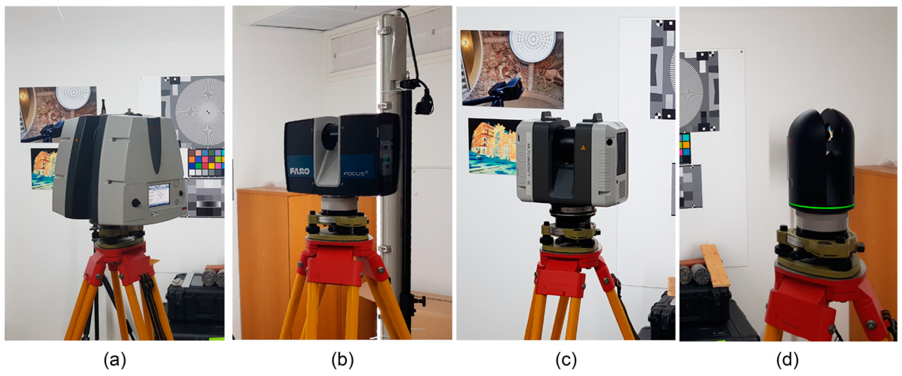
2.1. Tested Instruments

The test method was applied using four modern commercial panoramic TLS instruments: a Leica ScanStation P40 [68], a Faro Focus S 350 [19], a Leica RTC360 [18], and a Leica BLK360 [69] (Figure 2). These commercially available instruments represent diverse design choices, e.g., in their operating range, portability, affordability, and camera configurations and specifications. Specifications of the tested instruments are presented in

Table 1. Scanner specifications [18,19,68,69].

TLS System	Scan Rate	Ranging Method	Range Accuracy	Max Range	Wavelength	Beam Divergence	Weight (Incl. Battery)
Leica ScanStation P40	1,000,000 pts/s	Time-of-flight	1.2 mm + 10 ppm	270 m	1550 nm	<0.23 mrad (FWHM)	12.65 kg
Faro Focus S 350	976,000 pts/s	Phase based	1.0 mm	350 m	1550 nm	0.3 mrad (1/e)	4.2 kg
Leica RTC360	2,000,000 pts/s	Time-of-flight	1.0 mm + 10 ppm	130 m	1550 nm	0.5 mrad (1/e2, full angle)	5.64 kg
Leica BLK360	360,000 pts/s	Time-of-flight	4 mm @ 10 m	60 m	830 nm	0.4 mrad (FWHM)	1 kg

and

Table 2. Scanner imaging specifications [18,19,68,69].

TLS System	No. of Camera Sensors	Camera Configuration	Camera Sensor Resolution (Pixels)	No. of Photos Used for Equirectangular Panorama	Est. Total Raw Pixel Count for Single Exposure (Megapixels)	No. of Exposure Brackets for HDR Imaging
Leica ScanStation P40	1	Mounted coaxially with laser	1920 × 1920 1	260 [70]	958 3	3 [71]
Faro Focus S 350	1	Mounted coaxially with laser	3264 × 2448 2	66 3	527 3	2, 3, or 5
Leica RTC360	3	Mounted to scanner body	4000 × 3000 1	12 per camera 1	432 1	5
Leica BLK360	3	Mounted to scanner body	2592 × 1944 1	10 per camera 1	150 1	2, 3, 4, or 5

¹ Information from the manufacturers’ product specifications. ² Size of a single exported image frame. ³ Estimated from the data.

.

An additional photographic reference dataset was collected using a Nikon D800E digital single-lens reflex (DSLR) camera with a Nikkor AF-S 14–24 mm f/2.8G lens. The focal length was set to 14 mm. An aperture of f/5.6 was set to make the image as sharp as possible without the diffraction blurring effect, and an ISO speed of 100 was selected for minimal noise. The resolution of the camera sensor was 7360 × 4912 pixels. The purpose of this reference data set was to verify the test conditions with a known, calibrated camera and lens combination and to give a good indication of the achievable quality if an external camera were to be used for the point cloud colorization.

2.2. Test Environment

An indoor test environment was prepared for the TLS instruments, consisting of a blacked-out room with a lighting system, fixed scanner mounting position, and a set of horizontally mounted standardized test charts designed for testing various image quality factors related to color reproduction, sharpness, and noise (see Figure 3). In addition, a set of printed photographs were present in the scene.

The X-Rite ColorChecker Classic [72] color reference target (Figure 3a) was used to assess quality factors related to color reproduction, such as color accuracy. A standard size (21.6 × 27.9 cm) ColorChecker chart consists of 24 reference patches representing natural objects, as well as chromatic, primary, and grayscale colors.

The sinusoidally modulated Siemens star [73] chart (Figure 3b) was used to assess quality factors related to detail reproduction such as image sharpness. The Siemens star chart (size of 50.0 × 66.7 cm) consists of 144 pattern bands and is included in the ISO 12233:2017 [74] standard (Annex E). Measuring sharpness via resolution measurements using the sinusoidal Siemens star is considered a reliable approach for all cameras and is less susceptible to image processing (e.g., sharpening) compared to methods that rely on high contrast edges. Furthermore, it allows measuring sharpness from multiple angles at a time [73].

The simplified ISO 15739 digital camera noise test chart (Figure 3c) based on ISO 15739 [75] was used to quantify the amount of noise in the data. The noise test chart (size of 30.5 × 45.7 cm) consists of 15 uniform greyscale patches specially designed for measuring noise.

The test environment was illuminated with uniform the standard illuminant D65 (for noon daylight and sRGB) as specified in the ISO 11664-2:2007 standard [76]. D65 is highly compatible with the popular sRGB color space [77] that has a white point at a corresponding 6500 K temperature and is considered to be consistent among various devices (e.g., computers, cameras, monitors, and mobile devices), as well as the Internet and common 3D graphics programming interfaces such as Direct3D [78], OpenGL [79], and WebGL [80].

2.3. Data Acquisition

In the test environment, scans were obtained from a fixed scanning location using a fixed and leveled tripod height of 1.36 me at a distance of 2 m from the targeted image quality test charts. The tripod height was set approximately to the same level as the wall-mounted test charts. Due to the structural differences (e.g., shape, size, and sensor configuration) in the scanner systems, identical positions for the scanner optical centers were not achieved. The optical center heights were within approximately 7 cm from each other between the tested scanners.

Tested scan and imaging settings were set so that the total data collection time per station was reasonable considering the real-life use of the scanner in the field where a project can easily consist of tens or even hundreds of scan stations. Thus, data collection times above 20 min per station were avoided.

The scans were repeated using two alternative resolution settings to observe the effect of scan resolution: a high-density scan setting with the closest available setting to three millimeters at ten meters (see

Table 3. A summary of the acquired laser scans.

TLS System	Scan Resolution	Dynamic Range	Scan Time (min:s)	Imaging Time (min:s)	Total Time (min:s)
Leica ScanStation P40	3.1 mm @ 10 m	HDR	3:30	10:19	13:49
		LDR	3:30	7:22	10:52
	6.3 mm @ 10 m	HDR	1:49	10:19	12:08
		LDR	1:49	7:22	9:11
Faro Focus S 350	3.1 mm @ 10 m	HDR	15:19	11:25	26:44
		LDR	15:19	2:07	17:26
	6.1 mm @ 10 m	HDR	4:35	11:25	16:00
		LDR	4:35	2:07	6:42
Leica RTC360	3.0 mm @ 10 m	HDR	1:42	1:00	2:42
		HDR	0:51	1:00	1:51
Leica BLK360	5.0 mm @ 10 m	HDR	3:40	1:40	5:20
		LDR	3:40	1:00	4:40

) and a medium-density scan setting with the closest available setting to six millimeters at ten meters (see Table 3) as selectable in the scanner settings. These parameters were chosen because they were as equally reproducible as possible within all chosen scanner instruments and those also well represented assumed typical real-life use cases.

All the tested scanners were capable of capturing high dynamic range (HDR) images. Whenever possible the tests were repeated using both HDR and low dynamic range (LDR) imaging settings. The Leica RTC360 uses only HDR imaging without any option for LDR. With LDR we refer to non-HDR imaging where the dynamic range of the image data consists of an exposure time of a single image. Whenever possible, the varying imaging settings were set to represent the highest quality setting and as full automation as possible.

Some tested scanners had relevant user-controllable scan and imaging parameters that were tested and set according to the test environment and method. For the Leica ScanStation P40, the image resolution was set to maximum, the exposure time was set to automatic, the white balance adjustment was set to the “cold light” preset mode to match the scene lighting, and the scan sensitivity was set to “normal”. For the Faro S 350 the exposure metering mode was set to “even weighted metering”, the HDR images were collected with the maximum number of five brackets, and the scan quality setting (which reduces the level of noise in the distance measurement at the cost of increasing the scanning time) was set to “3x”. The photographic reference dataset was captured from the same location with the scans in the NEF (Nikon electronic file) format. A summary of the acquired scans and their selected comparable settings for assessing the point cloud colorization quality are listed in Table 3.

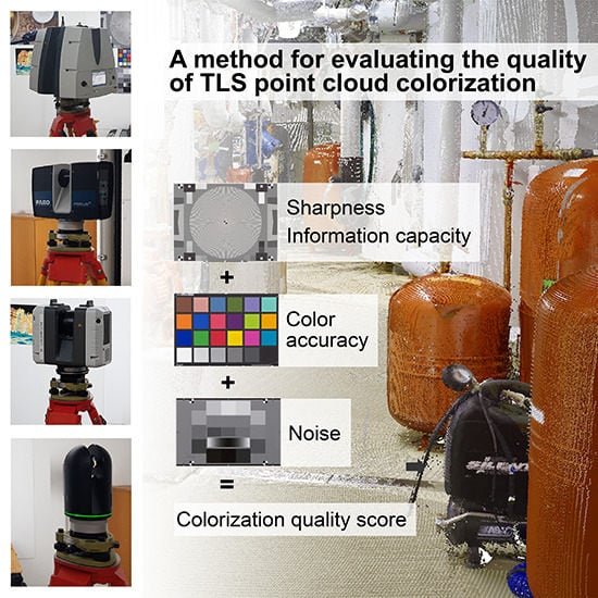
2.4. Developed Method in Brief

After the data acquisition phase, the 3D point cloud data sets were processed and analyzed for the purpose of evaluating the colorization quality. For this goal, a test method was developed to prepare 2D images from the 3D scanned test charts and analyze the resulting image data using selected image quality metrics that describe the capabilities of the scanner system to reproduce colors and details in the scene. To assess the usefulness of our method for benchmarking purposes, the results of these individual quality metrics were summarized into one combined quality score per scan. This proposed method for evaluating the colorization quality is introduced in detail in the next section (Section 3).

3. The Proposed Method for Evaluating the Colorization Quality of TLS-Derived 3D Point Clouds

To evaluate the point cloud colorization quality of the tested TLS systems, a test method was developed. The key purpose of this proposed method was to process, colorize, and prepare the 3D point clouds of the scanned image quality test charts into 2D images that could be analyzed using image quality measurements. Our test method was split into three stages: (1) point cloud pre-processing and colorization, (2) point cloud preparation for image quality analysis, (3) image quality analysis, and (4) combining metrics to achieve a final quality score. An overview of the developed method is illustrated in Figure 4.

3.1. Image Quality

Image quality is the result of a complex combination of quality factors inherited from the imaging sensor, the lens, and the image processing pipeline. Image quality can be assessed objectively by analyzing the image data via various automated image quality measurements, or subjectively by relying on various perceptual methods that assess human subjects [81]. For objective assessment there exists a great amount of literature and numerous standards (e.g., ISO 12233 [74] for resolution and spatial frequency response measurements, and ISO 15739 [75] for noise measurements) for testing various image quality aspects of digital cameras. These standards define a broad range of quality metrics that are typically calculated from a wide variety of different test charts, e.g., Siemens stars or slanted-edge charts for resolution measurements, and grayscale charts for noise. Image quality testing from these charts can be performed with applicable software, e.g., Imatest Master (Imatest LCC, Boulder, CO, USA) [82] or iQ-Analyser (Image Engineering GmbH & Co. KG, Kerpen, Germany) [83].

Sharpness, color reproduction, and noise have been regarded as the most important metrics of imaging quality (e.g., [62]), but no single metric exists that would depict the quality of a camera as a whole. Firstly, sharpness determines the amount of detail the imaging sensor can capture. For example, it can be objectively quantified with resolution measurements that define the sensor’s capability to maintain the optical contrast of increasingly finer details in a scene [84]. Secondly, color reproduction determines the ability of the imaging sensor to reproduce colors in the scene. An accurate color description can be understood as a truthful combination of chromatic and luminance components. Finally, noise can be described as unwanted random spatial variation in an image, and objective noise measurements are commonly based on measuring a signal-to-noise ratio from an image.

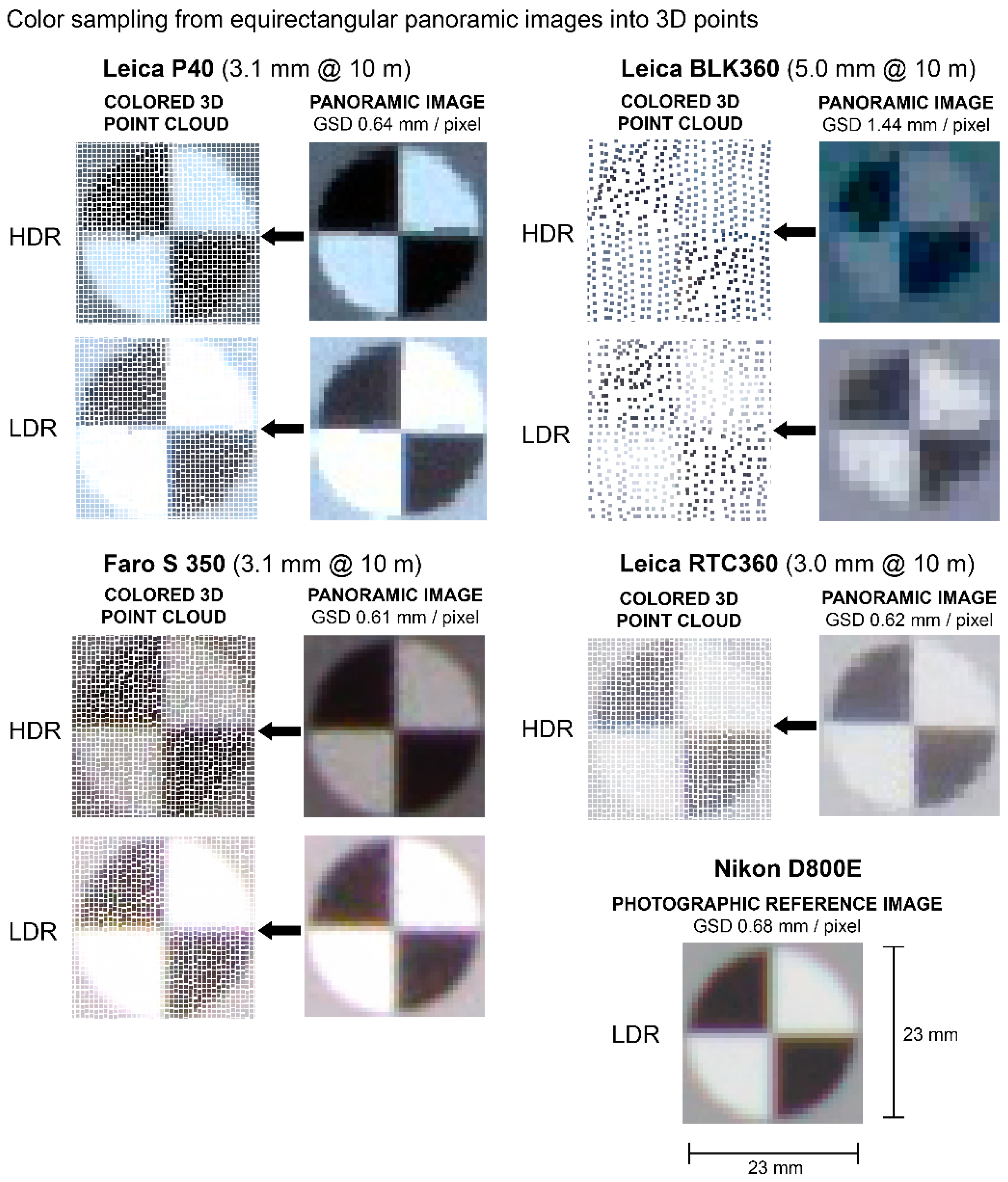
3.2. Point Cloud Pre-Processing and Colorization

The point cloud pre-processing workflow (see Figure 4) consisted of processing the raw scan data and colorizing the point clouds. The raw laser scan data was processed with respective original software from the scanner manufacturers (Leica Cyclone REGISTER 360 version 1.6.2. [85] and Faro SCENE version 7.5.2.3361 [86]). Both manufacturers’ software included various optional features to adjust the image data prior to the point cloud colorization. This included support for exporting the panoramic images for editing with third-party software, tools to semi-automatically tune the white balance, and several alternative tone mapping operators that are used to map the HDR image data to more limited dynamic ranges that are universally supported by typical devices and displays.

For LDR scans, all scans were colorized using the suggested default settings to achieve as straightforward and automated results as possible that would depict the most typical colorized point cloud output from the given scanner.

For HDR scans, two alternative strategies were employed. Firstly, the scans were colorized using the default settings in the software similarly to LDR. Alternatively, the resulting raw equirectangular panoramic photos were also tone mapped using a linear operator, and then the exposure and white balance levels were manually set in an external program Darktable (version 3.0.0), an open-source program for editing raw photographs [87]. The idea of this alternative approach was to process the raw image data with an equal workflow to mitigate the unknown effects of automated image processing in point cloud colorization. In general, the purpose of a tone mapping operator is to compress the luminance range (e.g., from 32-bit into 8-bit per channel) while preserving contrast [88]. There exist a wide range of different tone mapping operators but validating and comparing their performance is considered difficult [89] and was considered beyond the scope of this work. Thus, a linear tone mapping operator was selected as the most consistent alternative between the tested scanners. Firstly, 32-bit raw panoramic image files were exported (as .exr files from the Leica Cyclone REGISTER 360 and as .hdr files from the Faro SCENE) using linear tone mapping settings. Secondly, the image exposure and white balance were manually edited in Darktable and finally, the images were exported as 8-bit JPEG image files in sRGB color space for subsequent colorization in the Leica and Faro software.

For both the LDR and HDR scans, the resolution of the equirectangular panoramic images was set as large as possible for the maximum level of detail in the point cloud colorization. For Leica ScanStation P40 and RTC360 scanners, the resolution was set to the maximum of 20,480 × 10,240 pixels, and with Faro Focus S 350 the maximum value of 20,288 × 10,144 was used. For the Leica BLK360, the default resolution setting of 8192 × 4096 was selected because the estimated total pixel count per scan was not considered feasible to produce a panoramic photo with the same maximum resolution (of 20,480 × 10,240 pixels) without oversampling and thus potentially producing biased test results.

Finally, the colorized point clouds were exported in the E57 format containing location (XYZ) and color (eight-bit per channel RGB) information in sRGB color space.

3.3. Point Cloud Preparation for Image Quality Analysis

Colorized point cloud data per each tested scanner was prepared using CloudCompare (version 2.10-alpha), which is an open-source 3D point cloud and mesh model processing software package [90]. The goal was to prepare and render comparable 2D image files from colorized 3D point cloud data for each test chart for further image quality analysis. This data preparation workflow (illustrated in Figure 4) was as follows:

1.

3D points representing each test chart were manually segmented from the point clouds.

2a.

The points representing the ColorChecker were rendered as point clouds using rectangular points with the point size set to the minimum so that there were no visible holes inside the charts. This was done to mitigate any interpolation of color data before the color-related quality measurements.

2b.

Alternatively, for the points representing the Siemens star chart and the simplified ISO 15739 digital camera noise test chart, a Delaunay triangulation was performed to create mesh models (with vertex colors) of the charts. This was done to fill all potential gaps in the point cloud and to negate the effect of point size for the detail reproduction-related quality measurements.

3.

The segmented test charts were rendered using orthographic projection and an equal zoom level between the charts and exported as 2D image files in PNG format.

3.4. Image Quality Analysis

The rendered 2D images of the 3D scanned test charts were analyzed using Imatest Master (version 2020.1.0.45711 Alpha), a software package for analyzing image quality factors [82]. The eight-bit (per channel) image files (in sRGB color space) processed from colorized 3D point cloud data per each respective image quality chart were used as input data for image quality analysis (see Figure 4).

Prior to the analysis, the photographic reference image collected with the Nikon D800E was converted in Darktable into a 16-bit TIFF file from the raw NEF format using AmaZe de-mosaicking algorithm, and scene-specific exposure and white balance levels were adjusted without any artificial sharpening or denoising.

3.4.1. Color Reproduction

A Color/Tone module [91] in Imatest was used to calculate the color accuracy from the ColorChecker charts for each scan. Algorithms used by Imatest are described in detail in [92]. CIEDE2000 color difference formulas [93], also part of the ISO/CIE 11664-6:2014 standard for colorimetry [94], were used to calculate the mean color difference ΔE₀₀ and chroma difference ΔC₀₀. The CIEDE2000 formula is considered to be the most accurate color differencing equation (e.g., [95,96]). Compared to the total color difference (ΔE₀₀), the chroma difference (ΔC₀₀) describes color accuracy as an error in colorfulness where the effects of exposure errors are reduced (indicated by differences in luminance) [92]. As additional metrics, the exposure and white balance error were calculated from the grayscale patches of the ColorChecker chart using the calculation methods described in [92].

3.4.2. Detail Reproduction

A Star Chart module [97] in Imatest was used to measure the instrument’s capability to reproduce details in the scene. The sharpness (modulation transfer function, MTF) and Shannon information capacity were calculated from the sinusoidally modulated Siemens star chart for each tested scan.

The sharpness can determine the maximum level of detail that the imaging system is able to capture. As a metric for system sharpness, the MTF was measured as a mean from the star pattern along the radii of a circle in eight segments. MTF is often interchangeably referred to as a spatial frequency response (SFR). For comparison purposes, spatial frequencies of MTF50P and MTF10P were selected as metrics to summarize the MTF curves. MTF50P describes a spatial frequency where the image contrast drops to 50% of its peak value and it is less sensitive to artificial image sharpening and can provide a more stable indication of the system performance than other similarly used metrics [98]. MTF10P describes a spatial frequency where the image contrast drops to 10% of its peak value and it is considered to correspond to a limiting resolution below which all information can be considered useless. Algorithms for calculating the MTF from a Siemens star in Imatest are based on [73] and the ISO 12233 standard [74].

In addition to assessing the sharpness by measuring the MTF values, the Shannon information capacity [99] was tested as an experimental image quality metric to measure the information capacity in bits per pixel for each scan. It is a novel metric introduced in Imatest and based on the original Shannon information capacity theory [100] with the hypothesis that image sharpness (MTF) and noise correlate to the information capacity that is proportional to the perceived image quality. The sinusoidal Siemens star is a recommended test chart for calculating the Shannon information capacity because it allows the signal (proportional to MTF) and noise to be calculated from the same location. The method used by Imatest is described in detail by [101].

Noise can be described as undesirable random spatial variation in an image that obscures desired details. To quantify the level of noise a signal-to-noise ratio (SNR) was calculated according to the ISO 15739 [75] standard using the Color/Tone module [91] in Imatest. The SNR was calculated from the uniform gray patches of the simplified ISO 15739 grayscale noise test chart for each scan. The calculation method is described in detail in [102].

3.5. Combining Metrics for a Quality Score

For the purpose of benchmarking, the individual calculated quality metrics were combined to form a comparable quality score per scan. To achieve this, we recognized that geometric means have been described as suitable averaging approaches to combine a wide range of measurements even without normalization [103,104]. For example, [62] used geometric means to combine camera phone image quality and performance metrics into one benchmark score. Similar to this, the point cloud colorization quality score per scan was calculated as a geometric mean of the selected quality metrics using the following Equation (1):

Quality Score = ⁶√ (MTF50P × MTF10P × C × SNR × 1/ΔE₀₀ × 1/WBerr),

(1)

The measured results of system sharpness (summarized as MTF50P and MTF10P), Shannon information capacity (C), signal-to-noise ratio (SNR), color difference (ΔE₀₀), and white balance error (WBerr) were combined into one benchmarking score. The quality score combines these individual quality metrics that describe the instrument’s capability in reproducing color and details from the scene in the form of RGB color values of a 3D point cloud.

4. Results

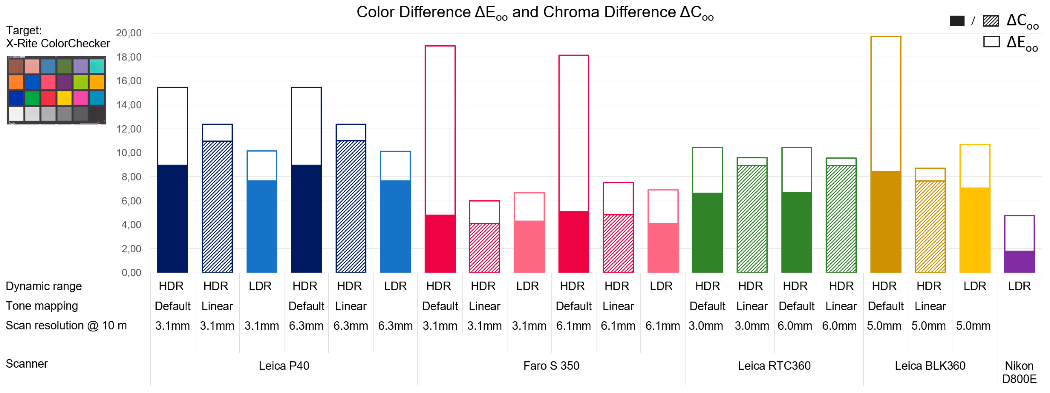
4.1. Color Reproduction

To evaluate the scanner systems’ ability to reproduce colors, the color accuracy was measured from colorized 3D point clouds representing the ColorChecker chart for each scan. Additional metrics of exposure error and the mean white balance error were also calculated. A table summarizing the results is presented in

Table A1. A summary of color reproduction metrics: the measured color accuracy, exposure error, and white balance error values for each tested scan.

Scan (Scanner, Dynamic Range, Scan Resolution, Tone Mapping)	Color Difference (Mean ΔE00)	Chroma Difference (Mean ΔC00)	Exposure Error (f-Stops)	White Balance Error (Saturation)
Leica P40, HDR, 3.1 mm, Default	15.48	9.04	−0.89	0.19
Leica P40, HDR, 3.1 mm, Linear	12.39	10.98	−0.45	0.08
Leica P40, LDR, 3.1 mm	10.16	7.72	0.85	0.14
Leica P40, HDR, 6.3 mm, Default	15.47	9.03	−0.84	0.18
Leica P40, HDR, 6.3 mm, Linear	12.40	11.02	−0.44	0.08
Leica P40, LDR, 6.3 mm	10.14	7.70	0.85	0.14
Faro S 350, HDR, 3.1 mm, Default	18.94	4.87	−1.22	0.05
Faro S 350, HDR, 3.1 mm, Linear	6.02	4.13	−0.05	0.02
Faro S 350, LDR, 3.1 mm	6.68	4.35	0.41	0.05
Faro S 350, HDR, 6.1 mm, Default	18.16	5.15	−1.03	0.05
Faro S 350, HDR, 6.1 mm, Linear	7.53	4.84	0.04	0.02
Faro S 350, LDR, 6.1 mm	6.92	4.15	0.6	0.04
Leica RTC360, HDR, 3.0 mm, Default	10.44	6.68	0.03	0.06
Leica RTC360, HDR, 3.0 mm, Linear	9.59	8.93	−0.10	0.08
Leica RTC360, HDR, 6.0 mm, Default	10.46	6.73	0.02	0.06
Leica RTC360, HDR, 6.0 mm, Linear	9.58	8.93	−0.16	0.08
Leica BLK360, HDR, 5.0 mm, Default	19.69	8.48	−1.71	0.33
Leica BLK360, HDR, 5.0 mm, Linear	8.72	7.66	−0.38	0.14
Leica BLK360, LDR, 5.0 mm,	10.69	7.11	−0.50	0.17
Nikon D800E photographic reference	4.77	1.86	−0.11	0.05

and the analyzed ColorChecker charts for each scan with high-resolution setting (closest to 3 mm @ 10 m) are listed for visual reference in

Table A2. The analyzed ColorChecker charts (8-bit/sRGB) for each scan segmented from colorized 3D point clouds with high scan resolution setting (closest to 3 mm @ 10 m).

Leica P40 HDR (default tone mapping) 3.1 mm @ 10 m	Leica P40 HDR (linear tone mapping) 3.1 mm @ 10 m	Leica P40 LDR 3.1 mm @ 10 m
Faro S 350 HDR (default tone mapping) 3.1 mm @ 10 m.	Faro S 350 HDR (linear tone mapping) 3.1 mm @ 10 m.	Faro S 350 LDR 3.1 mm @ 10 m.
Leica RTC360 HDR (default tone mapping) 3.0 mm @ 10 m.	Leica RTC360 HDR (linear mapping) 3.0 mm @ 10 m.	LDR setting not available
Leica BLK360 HDR (default tone mapping) 5.0 mm @ 10 m.	Leica BLK360 HDR (linear tone mapping) 5.0 mm @ 10 m.	Leica BLK360 LDR 5.0 mm @ 10 m.

.

To quantify the total color accuracy, the mean values of absolute color difference (ΔE₀₀) for each scan are presented in Figure 5, below. Additionally, to assess the color accuracy with the minimum effect of luminance, the mean chroma difference (ΔC₀₀) was calculated for each scan. The color and chroma differences were calculated using the CIEDE2000 formulas [93]. For all of the tested scanners, the total color difference was the largest when using HDR mode with default tone mapping settings. The HDR scans acquired with the Leica RTC360 produced the smallest error when using these default settings. The results from the Faro S 350 were closest to the ColorChecker reference when the linear tone mapping settings were used or no HDR mode was used at all. As expected, the scan resolution setting did not show any significant effect on the color difference. For the chroma difference, using LDR produced generally more accurate chroma than using HDR. Of all tested scans, the Faro S 350 produced the smallest error while the Leica P40 had the largest differences in chroma values.

The measured exposure errors per scan are presented in Figure 6. The f-stop is the ratio between the focal length of the camera lens and the diameter of the entrance pupil. The HDR scans with default settings appeared to suffer from underexposure, except for the Leica RTC360 that produced the most accurate exposure. All the LDR scans suffered from overexposure, except the one collected with the Leica BLK360.

The measured mean white balance errors per scan are presented in Figure 7. The HDR scan with default tone mapping settings scanned with the Leica BLK360 clearly has the largest white balance error, while the Faro S 350 had the most accurate white balance.

A comparison between the measured color and the reference color for each patch of the ColorChecker chart is presented in Figure 8, below. The comparison showed visually perceivable differences in the chroma, white balance, and luminance values between the different scans and settings.

4.2. Detail Reproduction

The selected quality metrics related to system sharpness and information capacity were measured from colorized 3D scans of the Siemens star chart. To estimate the level of noise in the colored point clouds, the signal-to-noise ratio according to ISO 15739 was measured from colorized 3D scans of the simplified ISO 15739 noise test chart for each scan. A summary of the results is presented in

Table A3. A summary of the selected metrics for describing scanner systems’ ability to reproduce details: the measured system sharpness summarized as MTF50P and MTF10P, the Shannon information capacity, and the ISO 15739 signal-to-noise ratio for each tested scan.

Scan (Scanner, Dynamic Range, Scan Resolution, Tone Mapping)	MTF50P (Cycles/Pixel)	MTF10P (Cycles/Pixel)	Shannon Information Capacity (Bits/Pixel)	ISO 15739 SNR (dB)
Leica P40 HDR 3.1 mm Default	0.199	0.4	1.32	27.4
Leica P40 HDR 3.1 mm Linear	0.191	0.357	0.83	46.4
Leica P40 LDR 3.1 mm	0.255	0.468	1.32	15.6
Leica P40 HDR 6.3 mm Default	0.167	0.316	1.07	27.2
Leica P40 HDR 6.3 mm Linear	0.173	0.299	0.81	47.5
Leica P40 LDR 6.3 mm	0.201	0.353	1.04	15.6
Faro S 350 HDR 3.1 mm Default	0.237	0.419	2.21	26.8
Faro S 350 HDR 3.1 mm Linear	0.237	0.417	2.31	38.5
Faro S 350 LDR 3.1 mm	0.225	0.406	2.41	28.5
Faro S 350 HDR 6.1 mm Default	0.191	0.336	1.34	27.8
Faro S 350 HDR 6.1 mm Linear	0.196	0.339	1.38	40.1
Faro S 350 LDR 6.1 mm	0.190	0.328	1.45	30.4
Leica RTC360 HDR 3.0 mm Default	0.222	0.373	1.15	40.0
Leica RTC360 HDR 3.0 mm Linear	0.217	0.377	1.16	32.5
Leica RTC360 HDR 6.0 mm Default	0.188	0.312	0.97	41.0
Leica RTC360 HDR 6.0 mm Linear	0.182	0.31	0.83	34.0
Leica BLK360 HDR 5.0 mm Default	0.135	0.226	1.08	33.3
Leica BLK360 HDR 5.0 mm Linear	0.136	0.227	0.76	39.5
Leica BLK360 LDR 5.0 mm	0.129	0.206	0.81	31.5
Nikon D800E photographic reference	0.212	0.357	2.89	34.0

in the appendices and for visual reference, the analyzed Siemens star charts and the simplified ISO 15739 noise test charts per scan segmented from colorized 3D point clouds with high-resolution settings (the closest to 3 mm @ 10 m) are listed in

Table A4. The analyzed Siemens star charts (8-bit/sRGB) for each scan segmented from colorized 3D point clouds with high scan resolution setting (closest to 3 mm @ 10 m).

Leica P40 HDR (default tone mapping) 3.1 mm @ 10 m	Leica P40 HDR (linear tone mapping) 3.1 mm @ 10 m	Leica P40 LDR 3.1 mm @ 10 m
Faro S 350 HDR (default tone mapping) 3.1 mm @ 10 m	Faro S 350 HDR (linear tone mapping) 3.1 mm @ 10 m	Faro S 350 LDR 3.1 mm @ 10 m
Leica RTC360 HDR (default tone mapping) 3.0 mm @ 10 m	Leica RTC360 HDR (linear tone mapping) 3.0 mm @ 10 m	LDR setting not available
Leica BLK360 HDR (default tone mapping) 5.0 mm @ 10 m	Leica BLK360 HDR (linear tone mapping) 5.0 mm @ 10 m	Leica BLK360 LDR 5.0 mm @ 10 m

and

Table A5. The analyzed simplified ISO 15739 noise test charts (8-bit/sRGB) for each scan segmented from colorized 3D point clouds with high scan resolution setting (closest to 3 mm @ 10 m).

Leica P40 HDR (default tone mapping) 3.1 mm @ 10 m	Leica P40 HDR (linear tone mapping) 3.1 mm @ 10 m	Leica P40 LDR 3.1 mm @ 10 m
Faro S 350 HDR (default tone mapping) 3.1 mm @ 10 m	Faro S 350 HDR (linear tone mapping) 3.1 mm @ 10 m	Faro S 350 LDR 3.1 mm @ 10 m
Leica RTC360 HDR (default tone mapping) 3.0 mm @ 10 m	Leica RTC360 HDR (linear tone mapping) 3.0 mm @ 10 m	LDR setting not available
Leica BLK360 HDR (default tone mapping) 5.0 mm @ 10 m	Leica BLK360 HDR (linear tone mapping) 5.0 mm @ 10 m	Leica BLK360 LDR 5.0 mm @ 10 m

in the appendices.

4.2.1. Sharpness

As a metric for system sharpness, MTF curves were measured from the sinusoidal Siemens star charts. As expected, the results (see Figure 10) showed a clear increase in sharpness when the scan resolution was increased. While the differences between the tested dynamic range settings were not so self-evident. The mean MTF curves for each scan for all the compared dynamic range settings are presented in Figure 9. When using LDR the Leica P40 produced the sharpest result of all compared scans with a noticeable improvement in sharpness compared to the HDR scans. As expected, using HDR with the linear dynamic range settings appeared to reduce the sharpness with all scanners. Overall, the Leica BLK360 clearly produced the least sharp results at all tested settings.

To summarize the system sharpness, the selected spatial frequencies of MTF50P and MTF10P for all tested scans are presented in Figure 10.

4.2.2. Information Capacity

The calculated Shannon information capacity per scan is described in Figure 11. Overall, the information capacity increased with the scan resolution. Amongst all the tested scans the Faro S 350 produced the highest information capacity, especially at a higher scan resolution. Further, the information capacity of the Leica BLK360 was the lowest of all the comparable tested scans.

4.2.3. Noise

The signal-to-noise ratio according to ISO 15739 was measured from colorized 3D scans of the simplified ISO 15739 noise test chart per each scan and the results are described in Figure 12. Linear tone mapping improved SNR in all scans except the ones acquired with the Leica RTC360. The Leica P40 produced better results with default HDR than with LDR. On the other hand, using LDR improved the results with the Faro S350 and especially with the Leica BLK360.

4.3. Quality Score

The individual quality metrics for the color difference (ΔE₀₀), white balance error (WBerr), sharpness (MTF50P and MTF10P), Shannon information capacity (C), and signal-to-noise ratio (SNR) were combined into a single quality score using Equation 1 and are presented in Figure 13. The results indicated that the Faro S 350 had the best colorization quality when using LDR or HDR with linear tone mapping. The Leica RTC360 produced the best colorization quality when using HDR with minimal manual processing steps (default tone mapping settings). The Leica BLK360 produced the lowest quality score for all tested settings. Using linear tone mapping appeared to increase the colorization quality for all the scanners except for the Leica RTC360. In addition, the scan resolution increase improved the colorization quality for all tested scanners.

5. Discussion

We implemented a method to assess the point cloud colorization quality of modern commercial TLS systems with integrated imaging sensors. The capabilities to reproduce colors and details were investigated by applying established image quality assessment methods. The results showed clear differences between the tested scanners in all measured quality aspects and can be supported well with visual observations. These measured and perceived quality inconsistencies in point cloud colorization reduce the reliability and usefulness of the color information and can hinder the ability to produce uniform color information between different scan settings and scanners. With this research, we hope to raise the awareness of the importance of the quality of point cloud colorization and its implications on applications that rely on colored 3D point clouds. Better colorization quality leads to higher quality interpretation and analyses, and potentially increases the level of automation in various data processing and modeling tasks.

The established objective image quality metrics were successfully implemented and appear to be useful in evaluating TLS colorization quality even in the case where the quality of an imaging system is a complex combination of an unknown number of unknown factors related to the quality of the lens, imaging sensor, image processing (e.g., compression, tone mapping, sharpening, noise removal, panoramic stitching, and point cloud colorization) and the test chart. Nevertheless, our method can be considered suitable for comparing all TLS instruments even those which are essentially “black box” types of systems, or those that rely on an external camera for point cloud colorization. Yet we hope to encourage scanner manufacturers to be more open about the imaging capabilities and specifications of their scanners. This would not only help in fixing the found errors and inconsistencies in the colorization but would assist in making better and more proven decisions on instrument selection. Additionally, at least for many scientific applications, fully controllable measurement parameters would be highly beneficial. The results suggest that the problems in the reproduction of color could be mitigated in data processing while the issues related to the reproduction of details such as sharpness or noise are much more beyond the control of a user.

5.1. Color Reproduction

Furthermore, the measured and visually clearly detectable errors (e.g., reported in real-life conditions by [58]) in luminance caused by the inaccurate exposure time and white balance can be corrected using semi-automated or manual adjustments similar to those commonly used in editing photographs. Tools to correct these types of errors are already offered by the scanner manufacturers but their use can be discouraged due to lack of awareness and knowledge caused by vague settings and insufficient documentation, or the significantly increased workload when editing data of larger measuring campaigns from multiple scanning stations. In addition to the luminance, properly correcting the chroma error and verifying the corrections would require the scanner to be color calibrated in the field with a color reference chart like the ColorChecker and applicable tools (similarly to the color corrections done for a photogrammetric data set by [2]). This color calibration would improve the quality of the colored 3D point cloud data, but also the collected panoramic images that could also be used directly e.g., as a data source in virtual tour applications or in illuminating virtual scenes with HDR image-based lighting.

Lighting conditions have a significant impact on the colorization quality. In even and stable lighting conditions, such as in our test environment, using the HDR mode to colorize the scans appears to offer few benefits if the colorization is done with the default settings and without any scene-specific manual adjustments. On the contrary, scans colorized using LDR image data appeared to produce better results than the default HDR workflows. However, HDR can be expected to be much more beneficial in challenging real-life circumstances with changing and uneven lighting, such as in typical outdoor environments. It is also notable that all the tested point clouds included color information of eight-bits per channel, which does not exploit the full potential of HDR and thus favors LDR. Automatically compressing the luminance range from 32-bits to 8-bits per channel causes inaccuracies in the color data, but 8-bits per channel is arguably the most widely used and supported format for storing the color information in point clouds and displaying and handling it in various applications and viewers.

By processing the HDR data alternatively with linear settings we were able to assess the colorization quality with fewer unknown image processing steps compared to automated tone mapping. The clear improvement in quality between the default and linear tone mapping settings suggests that there is potential to achieve a better colorization quality by improving or optimizing the automated image processing pipeline.

On the other hand, the goal of these automated processes could be to produce more visually appealing colors than accurate ones. When speaking of color, it is crucial to note the difference between accurate and visually pleasing color. Automatic image processing is typically aimed towards providing pleasing color via processes such as saturation boosting and artificial sharpening. However, in many applications, especially in remote sensing, the truthful and unmodified presentation of radiometric values can be considered more important and useful than visual appearance (e.g., [105]), and even a precondition for some use cases such as imaging luminance measurement (e.g., [106]). Furthermore, it is arguably easier to adjust accurate colors to be visually pleasing than adjusting visually pleasing colors to be accurate.

The challenges in automated and scene-specific processing can be underlined with the observable errors in sharpness, colorfulness, exposure, and white balance between the tested scans as seen in Figure 14.

5.2. Detail Reproduction

A scanner’s capability to reproduce details that transfer into color information is a complex combination of factors affected, e.g., by the scan resolution and the resolution of the images the color information is transferred from. In practice, the smallest detectable detail is governed by the sampling distance of both the laser and the camera sensor and, e.g., interpolation is required if the image resolution is not high enough. Additionally, the overlap required by the panoramic stitching affects the sampling. Thus, compared to color reproduction, assessing the factors related to detail is perhaps even more complex and difficult to measure, and moreover, to correct.

An illustration of how color values are sampled from equirectangular panoramic images into 3D point clouds is presented in Figure 15. Further, the ground sample distance (GSD) of the image data can be estimated using the physical size of the center circle (with a diameter of 23 mm) of the Siemens star chart to give a better picture of the limitations in transferring details from the image data into the 3D point cloud.

Increasing the scan resolution unsurprisingly increased the level of measurable details, but the tested dynamic range settings appeared to show variable effects. This can be explained by unknown processing steps, such as sharpening or noise reduction, in the image processing pipeline. The measured sharpness and visual observations suggest that especially the data collected with the Leica P40 was affected by strong artificial sharpening. This can be seen as clearly visible halo effects in the edges and is mitigated in the linear processed HDR datasets (Figure 16).

The calculated Shannon information capacity indicated the superior quality of the Faro S 350 and the photographic reference dataset. In theory, this novel image quality metric could be the best single quality metric to describe the potential detail reproduction of the whole system since it takes both sharpness (i.e., MTF) and noise into account and measures both from the same location. The measured results appear to be more in line with the visual observations than relying solely on single MTF measurements or a signal-to-noise ratio that on their own seem to be more sensitive to image processing.

All the tested scans were measured to be unsharp (or blurred) and especially the scans by the Leica BLK360 were significantly more blurred compared to the other tested scans. This was caused, at least partially, when some of the details were transferred in the colorization process from pixels into 3D points and then the 3D point data was transformed back into 2D image files where the gaps between the points were filled with interpolated values. This interpolation effect is stronger the lower the point density is. Thus, this data preparation process in effect denoises the analyzed images and to some degree proportionally favors the lowest resolution Leica BLK360 in the SNR measurements.

5.3. The Photographic Reference Dataset

As expected, the Nikon D800E DSLR camera produced a better-combined quality score than all the scanners and the best overall color reproduction quality. On the other hand, the TLS scanners performed better at reproducing details than had initially been expected and in some cases (see Figure 10) exceeded the measured sharpness of the reference. However, the comparison between the scans and the photographic reference can be considered somewhat unreliable due to the inevitable differences in the data preparation, where a single photograph was analyzed directly instead of an image rendered from a 3D point cloud. Additionally, the selected 14 mm lens (used typically for photogrammetric applications) resulted in a much wider field of view (approximately 81.2° × 104.1°) when compared to the scanners (e.g., 48° × 62° with Leica RTC360) from identical distances to the target. This favored the scanners, especially in the detail reproduction measurements.

From the imaging perspective, using a handheld camera allows more flexibility in selecting a desirable and optimal point-of-view, whereas TLS is tied into a more limited number of fixed locations that are typically governed by the requirements and limitations of laser scanning. Yet, the results might further indicate that it is not inevitable that using an external camera would result in better colorization quality than that obtained from integrated camera sensors. Especially if scene-specific manual adjustments are made to the images collected by the scanner prior to colorization.

5.4. The Effect of Data Collection Speed

When assessing the colorization performance of a terrestrial laser scanner, the speed of the data acquisition cannot be neglected. The speed of a TLS instrument depends on the selected scan and imaging settings (e.g., scan resolution and dynamic range settings such as the number of exposure brackets with HDR) and the performance of the instrument. Long data collection times can not only increase the duration and cost of the real-life projects but also reduce the quality of the collected data via changes in the environment and its lighting such as changing weather conditions or moving objects in the scene.

In this study, the differences between the data acquisition times were strikingly different with possible real-life implications. When collecting HDR data at high scan resolutions (closest to 3.0 mm @ 10 m) the fastest tested scanner (the Leica RTC360 at 2 min 42 s) was ten times faster than the slowest scanner (the Faro S 350 at 26 min 44 s) with equivalent settings. To some degree, the scan time of the Faro S 350 was longer because a quality setting of “3x” had to be used that reduced noise in the distance measurement data and make sure that there were no gaps in the point cloud data. Two of the fastest scanners (the Leica RTC360 and Leica BLK360) use three camera sensors mounted on the scanner body, instead of the more traditional approach where the scene is imaged through a single camera mounted coaxially with the laser. When collecting HDR image data, the imaging time is also affected by the exposure bracketing settings. The Leica P40 collected three brackets, whereas all the other instruments collected five.

Furthermore, in real-life situations in the field, the imaging time could make a difference as to whether to use HDR or LDR mode. For example, with the Faro S 350 took 2 min and 7 s to acquire the LDR images, while collecting the HDR data took 10 min and 19 sec. Hence, this was 8 min and 12 s (487%) more time per scan, and this starts to accumulate if multiple scan stations are required. Furthermore, it would suggest that the decisions made about imaging have a larger impact on the total data acquisition time than those made about the actual laser scanning. The only exception being the scans collected at the high-resolution setting of the Faro S 350 where the scan duration was significantly longer than with the other tested scanners.

The relation between the quality score and scanning speed is further illustrated in Figure 17. Where the scanning speed was calculated as an inverse of the total scan time for each tested scan at a high scanning resolution (closest to 3.0 mm @ 10 m). Like the importance of colorization quality, the importance of the instrument speed also depends on the type of use case and the nature of the project.

5.5. Study Limitations

Our method assesses the colorization quality by analyzing the results of the 3D point cloud colorization process. Thus, it reflects the real-life situation where a colored 3D point cloud data is directly visualized or used in any application. The tests did not include raw panoramic pictures. While it would have given a better indication of the potential imaging quality it did not reflect the final point cloud colorization quality that well. Furthermore, the raw image data of single image frames could not be taken into account since that was not equally available from the different scanners we tested. Additionally, the effect of color blending that could cause potential artifacts between multiple scan stations was not taken into account.

In practice, testing all the possible image quality metrics was not feasible. Therefore, we selected those metrics that we assumed to be most suitable for describing the colorization quality of TLS-based 3D point clouds. Furthermore, our method combines individual quality metrics to form a comparable quality score and treats all selected quality metrics as equally important and includes no weighting. The use of a geometric mean was observed to be suitable for this purpose.

Furthermore, since the evaluation was based on the results of a complex chain of processes done in the scanner and later in the manufacturer’s software, the results may be subject to change based on the software and firmware versions.

5.6. Future Research Directions

Future research topics include the radiometric calibration of TLS instruments from the perspective of point cloud colorization, using a similar approach to evaluate the colorization quality of photogrammetric 3D point clouds, or point clouds colorized with an external camera. Further, multispectral or hyperspectral laser scanning holds great potential for removing the need for additional camera sensors in laser scanning altogether. Combining the intensity data of multiple wavelengths could be used to produce the color information for 3D point clouds directly and actively, as well as to advance existing applications (e.g., automated classification of materials) or create completely new applications (e.g., illumination independent texturing). Despite its promise, multispectral and hyperspectral laser scanning is still in its early stages with operational sensors existing mostly as research prototypes.

In general, the application space of 3D point cloud data is expected to increase in the future, using point clouds more and more directly without complex meshing or vectorization workflows. As an example, recent advances in point-based rendering are enabling the direct use of colored 3D point clouds in real-time rendered environments such as in-game engines (e.g., Unreal Engine [107]) or on the web (e.g., Potree [108]).

In luminance measurement, the photography parameters should be fully controllable and should preserve the captured data unchanged [109]. The TLS systems could be applied to measure a 3D luminance model to be used by architects, lighting designers, or illumination engineers. However, uncontrollable or automatic exposure makes the data useless for luminance measurement. Furthermore, certain common post-processing practices, such as unsharp masking or compressing the luminance range (bit-depth) makes the data worse for luminance measurement. High fidelity in color capturing, and controllable imaging would also be essential when TLS is used to capture data for surface material classification. In surface material classification, both the color and the luminance data are important. As the measurement direction is known, an alteration in luminance data can be applied in order to determine the specularity and the diffusivity parameters of the surface.

6. Conclusions

Despite the widespread application and indisputable usefulness of colored point clouds, insufficient attention has been put into investigating the colorization quality of TLS-derived 3D point clouds. Previous quality studies related to TLS data have focused largely on various aspects of geometric quality or on the quality of the point intensity values.

We successfully developed a test method to evaluate the point cloud colorization quality of modern commercial TLS systems with integrated imaging sensors. Our method assessed the capability of the tested scanner systems to reproduce colors and details of the scene by measuring the objective image quality metrics: color accuracy (ISO/CIE 11664-6), sharpness (ISO 12233), information capacity, and signal-to-noise ratio (ISO 15739) from test charts (X-Rite ColorChecker, sinusoidal Siemens star (ISO 12233), and a simplified noise test chart (ISO 15739)). Furthermore, the individual quality measurements were summarized into one combined quality score to demonstrate the usefulness of our method in benchmarking the colorization quality of any TLS instrument.

Our study found clearly noticeable quality issues in the tested 3D point clouds that reflect considerable differences between the tested terrestrial laser scanners: the Leica ScanStation P40, Faro Focus S 350, Leica RTC360, and Leica BLK360. The Faro S 350 produced the best colorization quality results when using LDR imaging mode or HDR with linear tone mapping. The Leica RTC360 performed the best when using HDR with default tone mapping settings, and the Leica BLK360 produced the lowest quality score among all tested settings. The results were in line with visual observations and suggest that the problems in color reproduction (i.e., measured differences in color, white balance, and exposure) could be mitigated in data processing, while issues related to detail reproduction (i.e., measured sharpness and noise) are more beyond the control of the scanner user. However, the processes and tools related to fixing these problems (e.g., in-field color calibration) have not yet either been well-established or would be labor-intensive to apply in a real-life project setting. Furthermore, the data acquisition times were significantly different between the tested scans and scanners (e.g., there was a 10× difference between the fastest scanner Leica RTC360 and the slowest scanner Faro Focus S 350). This has implications on the real-life performance of the instruments, and it is often the decisions made about the imaging settings (e.g., whether to use HDR or LDR) that have the greatest impact on the total data acquisition time spent in the field.

Despite being increasingly efficient and accessible measuring instruments, there is a need to develop better and more accessible colorization tools and workflows, and automated image processing pipelines that would increase not only the quality but also the production efficiency of 3D point cloud colorization. This focus on colorization quality would increase the direct applicability of colored 3D point clouds in various visually and radiometrically demanding use cases that require reliable object interpretation and recognition, visual analysis, or photorealism. Further, in many remote sensing related applications, the truthful and unmodified presentation of radiometric values can be considered more important and useful than visual appearance. This development would be relevant and useful not only in traditional application areas such as engineering, surveying, or cultural heritage but increasingly in emerging application fields such as virtual production in the film industry or 3D content creation for video games and immersive experiences.

References

- Lensch, H.P.; Kautz, J.; Goesele, M.; Heidrich, W.; Seidel, H.P. Image-based reconstruction of spatial appearance and geometric detail. ACM Trans. Graph. 2003, 22, 234–257. [Google Scholar] [CrossRef] [Green Version]
- Gaiani, M.; Apollonio, F.I.; Ballabeni, A.; Remondino, F. Securing color fidelity in 3D architectural heritage scenarios. Sensors 2017, 17, 2437. [Google Scholar] [CrossRef] [PubMed] [Green Version]
- A13.1-Scheme for the Identification of Piping Systems-ASME. Available online: https://www.asme.org/codes-standards/find-codes-standards/a13-1-scheme-identification-piping-systems (accessed on 25 June 2020).
- Virtanen, J.-P.; Daniel, S.; Turppa, T.; Zhu, L.; Julin, A.; Hyyppä, H.; Hyyppä, J. Interactive dense point clouds in a game engine. ISPRS J. Photogramm. Remote Sens. 2020, 163, 375–389. [Google Scholar] [CrossRef]
- Statham, N. Use of photogrammetry in video games: A historical overview. Games Cult. 2018, 15, 289–307. [Google Scholar] [CrossRef]
- Pepe, M.; Ackermann, S.; Fregonese, L.; Achille, C. 3D Point cloud model color adjustment by combining terrestrial laser scanner and close range photogrammetry datasets. In Proceedings of the ICDH 2016: 18th International Conference on Digital Heritage, London, UK, 24–25 November 2016; pp. 1942–1948. [Google Scholar]
- Gómez-Moreno, H.; Maldonado-Bascón, S.; Gil-Jiménez, P.; Lafuente-Arroyo, S. Goal evaluation of segmentation algorithms for traffic sign recognition. IEEE Trans. Intell. Transp. Syst. 2010, 11, 917–930. [Google Scholar] [CrossRef]
- Wang, Q.; Cheng, J.C.; Sohn, H. Automated Estimation of Reinforced Precast Concrete Rebar Positions Using Colored Laser Scan Data. Comput. Aided Civ. Infrastruct. Eng. 2017, 32, 787–802. [Google Scholar] [CrossRef]
- Yuan, L.; Guo, J.; Wang, Q. Automatic classification of common building materials from 3D terrestrial laser scan data. Automat. Constr. 2020, 110. [Google Scholar] [CrossRef]
- Valero, E.; Forster, A.; Bosché, F.; Hyslop, E.; Wilson, L.; Turmel, A. Automated defect detection and classification in ashlar masonry walls using machine learning. Automat. Constr. 2019, 106, 1–30. [Google Scholar] [CrossRef]
- Tutzauer, P.; Haala, N. Façade reconstruction using geometric and radiometric point cloud information. Int. Arch. Photogramm. Remote Sens. Spatial Inf. Sci. 2015, 40, 247–252. [Google Scholar] [CrossRef] [Green Version]
- Men, H.; Gebre, B.; Pochiraju, K. Color point cloud registration with 4D ICP algorithm. In Proceedings of the 2011 IEEE International Conference on Robotics and Automation (ICRA), Shanghai, China, 9–13 May 2011; IEEE: Piscataway, NJ, USA; pp. 1511–1516. [Google Scholar] [CrossRef]
- Łępicka, M.; Kornuta, T.; Stefańczyk, M. Utilization of colour in ICP-based point cloud registration. In Proceedings of the 9th International Conference on Computer Recognition Systems CORES 2015, Wroclaw, Poland, 25–27 May 2015; Springer: Berlin, Germany, 2015; pp. 821–830. [Google Scholar]
- Park, J.; Zhou, Q.Y.; Koltun, V. Colored point cloud registration revisited. In Proceedings of the 2017 IEEE International Conference on Computer Vision Workshop (ICCVW), Venice, Italy, 22–29 October 2017; IEEE: Piscataway, NJ, USA; pp. 143–152. [Google Scholar]
- Zhan, Q.; Liang, Y.; Xiao, Y. Color-based segmentation of point clouds. In Proceedings of the ISPRS Workshop Laserscanning ‘09, Paris, France, 1–2 September 2009; Bretar, F., Pierrot-Deseilligny, M., Vosselman, G., Eds.; pp. 155–161. [Google Scholar]
- Strom, J.; Richardson, A.; Olson, E. Graph-based segmentation for colored 3D laser point clouds. In Proceedings of the IROS 2010: IEEE/RSJ International Conference on Intelligent Robots and Systems, Taipei, Taiwan, 18–22 October 2010; IEEE: Piscataway, NJ, USA; pp. 2131–2136. [Google Scholar] [CrossRef] [Green Version]
- Verdoja, F.; Thomas, D.; Sugimoto, A. Fast 3D point cloud segmentation using supervoxels with geometry and color for 3D scene understanding. In Proceedings of the 2017 IEEE International Conference on Multimedia and Expo (ICME), Hong Kong, China, 10–14 July 2017; IEEE: Piscataway, NJ, USA; pp. 1285–1290. [Google Scholar] [CrossRef] [Green Version]
- Leica RTC360 3D Laser Scanner. Available online: https://leica-geosystems.com/products/laser-scanners/scanners/leica-rtc360 (accessed on 23 April 2020).
- FARO FOCUS LASER SCANNERS. Available online: https://www.faro.com/products/construction-bim/faro-focus/ (accessed on 23 April 2020).
- Trimble TX8 3D Laser Scanner. Available online: https://geospatial.trimble.com/products-and-solutions/trimble-tx8 (accessed on 23 April 2020).
- Z+F IMAGER 5016, 3D Laser Scanner. Available online: https://www.zf-laser.com/Z-F-IMAGER-R-5016.184.0.html?&L=1 (accessed on 23 April 2020).
- Pourreza-Shahri, R.; Nasser Kehtarnavaz, N. Exposure bracketing via automatic exposure selection. In Proceedings of the 2015 IEEE International Conference on Image Processing (ICIP), Quebec City, QC, Canada, 27–30 September 2015; IEEE: Piscataway, NJ, USA; pp. 2487–2494. [Google Scholar] [CrossRef]
- Trimble X7 3D Scanning System. Available online: https://geospatial.trimble.com/node/2650 (accessed on 23 April 2020).
- Gordon, S.; Lichti, D.D.; Stewart, M.P.; Tsakiri, M. Metric performance of a high-resolution laser scanner. Proc. SPIE 2000, 4309, 174–184. [Google Scholar] [CrossRef]
- Lichti, D.; Stewart, M.P.; Tsakiri, M.; Snow, A.J. Calibration and testing of a terrestrial laser scanner. Int. Arch. Photogramm. 2000, 33, 485–492. [Google Scholar]
- Boehler, W.; Vicent, M.B.; Marbs, A. Investigating laser scanner accuracy. Int. Arch. Photogramm. Remote Sens. Spatial Inf. Sci. 2003, 34, 696–701. [Google Scholar]
- Staiger, R. Terrestrial laser scanning technology, systems and applications. In Proceedings of the 2nd FIG Regional Conference, Marrakech, Morocco, 2–5 December 2003; pp. 1–10. [Google Scholar]
- Mechelke, K.; Kersten, T.P.; Lindstaedt, M. Comparative investigations into the accuracy behaviour of the new generation of terrestrial laser scanning systems. In Proceedings of the 8th Conference on the Optical 3-D Measurement Techniques, Zurich, Switzerland, 9–12 July 2007; Gruen, A., Kahmen, H., Eds.; Volume 3, pp. 19–327. [Google Scholar]
- Pfeifer, N.; Briese, C. Geometrical aspects of airborne laser scanning and terrestrial laser scanning. Int. Arch. Photogramm. Remote Sens. Spatial Inf. Sci. 2007, 36, 311–319. [Google Scholar]
- Wunderlich, T.; Wasmeier, P.; Ohlmann-Lauber, J.; Schäfer, T.; Reidl, F. Objective Specifications of Terrestrial Laserscanners—A Contribution of the Geodetic Laboratory at the Technische Universität München; Technische Universität München; Chair of Geodesy: Munich, Germany, 2013; pp. 1–38. [Google Scholar]
- Schmitz, B.; Holst, C.; Medic, T.; Lichti, D.D.; Kuhlmann, H. How to Efficiently Determine the Range Precision of 3D Terrestrial Laser Scanners. Sensors 2019, 19, 1466. [Google Scholar] [CrossRef] [Green Version]
- Lichti, D.D.; Jamtsho, S. Angular resolution of terrestrial laser scanners. Photogramm. Rec. 2006, 21, 141–160. [Google Scholar] [CrossRef]
- Ling, Z.; Yuqing, M.; Ruoming, S. Study on the resolution of laser scanning point cloud. In Proceedings of the 2008 IEEE International Geoscience and Remote Sensing Symposium, Boston, MA, USA, 8–11 July 2008; IEEE: Piscataway, NJ, USA; Volume 2, pp. 1136–1139. [Google Scholar] [CrossRef]
- Pesci, A.; Teza, G.; Bonali, E. Terrestrial laser scanner resolution: Numerical simulations and experiments on spatial sampling optimization. Remote Sens. 2011, 3, 167–184. [Google Scholar] [CrossRef] [Green Version]
- Clark, J.; Robson, S. Accuracy of measurements made with a Cyrax 2500 laser scanner against surfaces of known colour. Surv. Rev. 2004, 37, 626–638. [Google Scholar] [CrossRef]
- Kersten, T.P.; Sternberg, H.; Mechelke, K. Investigations into the accuracy behaviour of the terrestrial laser scanning system Mensi GS100. In Proceedings of the 7th Conference on the Optical 3-D Measurement Techniques, Vienna, Austria, 3–5 October 2005; Gruen, A., Kahmen, H., Eds.; Volume 1, pp. 122–131. [Google Scholar]
- Soudarissanane, S.; Van Ree, J.; Bucksch, A.; Lindenbergh, R. Error budget of terrestrial laser scanning: Influence of the incidence angle on the scan quality. In Proceedings of the 3D-NordOst 2007, Berlin, Germany, 6–7 December 2007; pp. 1–8. [Google Scholar]
- Voegtle, T.; Schwab, I.; Landes, T. Influences of different materials on the measurements of a terrestrial laser scanner (TLS). Int. Arch. Photogramm. Remote Sens. Spatial Inf. Sci. 2008, 37, 1061–1066. [Google Scholar]
- Soudarissanane, S.; Lindenbergh, R.; Menenti, M.; Teunissen, P. Scanning geometry: Influencing factor on the quality of terrestrial laser scanning points. ISPRS J. Photogramm. Remote Sens. 2011, 66, 389–399. [Google Scholar] [CrossRef]
- Kawashima, K.; Yamanishi, S.; Kanai, S.; Date, H. Finding the next-best scanner position for as-built modeling of piping systems. Int. Arch. Photogramm. Remote Sens. Spat. Inf. Sci. 2014, 40, 313–320. [Google Scholar] [CrossRef] [Green Version]
- Borah, D.K.; Voelz, D.G. Estimation of laser beam pointing parameters in the presence of atmospheric turbulence. Appl. Opt. 2007, 46, 6010–6018. [Google Scholar] [CrossRef] [PubMed]
- Bucksch, A.; Lindenbergh, R.; van Ree, J. Error budget of Terrestrial Laser Scanning: Influence of the intensity remission on the scan quality. In Proceedings of the Geo-Siberia 2007, Novosibirsk, Russia, 25–27 April 2007; pp. 113–122. [Google Scholar]
- Pfeifer, N.; Dorninger, P.; Haring, A.; Fan, H. Investigating Terrestrial Laser Scanning Intensity Data: Quality and Functional Relations. In Proceedings of the 8th Conference on Optical 3-D Measurement Techniques, Zurich, Switzerland, 9–12 July 2007; pp. 328–337. [Google Scholar]
- Kukko, A.; Kaasalainen, S.; Litkey, P. Effect of incidence angle on laser scanner intensity and surface data. Appl. Opt. 2008, 47, 986–992. [Google Scholar] [CrossRef] [PubMed]
- Kaasalainen, S.; Krooks, A.; Kukko, A.; Kaartinen, H. Radiometric calibration of terrestrial laser scanners with external reference targets. Remote Sens. 2009, 1, 144–158. [Google Scholar] [CrossRef] [Green Version]
- Krooks, A.; Kaasalainen, S.; Hakala, T.; Nevalainen, O. Correction of intensity incidence angle effect in terrestrial laser scanning. In Proceedings of the ISPRS Workshop Laser Scanning 2013, Antalya, Turkey, 11–13 November 2013; pp. 145–150. [Google Scholar] [CrossRef] [Green Version]
- Tan, K.; Cheng, X. Intensity data correction based on incidence angle and distance for terrestrial laser scanner. J. Appl. Remote Sens. 2015, 9. [Google Scholar] [CrossRef]
- Balaguer-Puig, M.; Molada-Tebar, A.; Marqués-Mateu, A.; Lerma, J.L. Characterisation of intensity values on terrestrial laser scanning for recording enhancement. Int. Arch. Photogramm. Remote Sens. Spatial Inf. Sci. 2017, XLII-2/W5, 49–55. [Google Scholar] [CrossRef] [Green Version]
- Hassan, M.U.; Akcamete-Gungor, A.; Meral, C. Investigation of terrestrial laser scanning reflectance intensity and RGB distributions to assist construction material identification. In Proceedings of the Joint Conference on Computing in Construction (JC3), Heraklion, Greece, 4–7 July 2017; pp. 507–515. [Google Scholar] [CrossRef] [Green Version]
- Abdelhafiz, A.; Riedel, B.; Niemeier, W. Towards a 3D true colored space by the fusion of laser scanner point cloud and digital photos. In Proceedings of the ISPRS WG V/4 3D-ARCH 2005: Virtual Reconstruction and Visualization of Complex Architectures, Mestre-Venice, Italy, 22–24 August 2005; El-Hakim, S., Remondino, F., Gonzo, L., Eds.; Volume XXXVI-5/W17. [Google Scholar]
- Forkuo, E.K.; King, B. Automatic fusion of photogrammetric imagery and laser scanner point clouds. Int. Arch. Photogramm. Remote Sens. Spat. Inf. Sci. 2014, 35, 921–926. [Google Scholar]
- Stal, C.; De Maeyer, P.; De Ryck, M.; De Wulf, A.; Goossens, R.; Nuttens, T. Comparison of geometric and radiometric information from photogrammetry and color-enriched laser scanning. In Proceedings of the FIG Working Week 2011: Bridging the gap between cultures, Marrakech, Morocco, 18–22 May 2011; International Federation of Surveyors (FIG): Copenhagen, Denmark; pp. 1–14. [Google Scholar]
- Moussa, W.; Abdel-Wahab, M.; Fritsch, D. An automatic procedure for combining digital images and laser scanner data. Int. Arch. Photogramm. Remote Sens. Spatial Inf. Sci. 2012, 39, 229–234. [Google Scholar] [CrossRef] [Green Version]
- Crombez, N.; Caron, G.; Mouaddib, E. 3D point cloud model colorization by dense registration of digital images. Int. Arch. Photogramm. Remote Sens. Spat. Inf. Sci. 2015, 40, 123–130. [Google Scholar] [CrossRef] [Green Version]
- Pleskacz, M.; Rzonca, A. Design of a testing method to assess the correctness of a point cloud colorization algorithm. Arch. Fotogram. Kartogr. i Teledetekcji 2016, 28, 91–104. [Google Scholar]
- Gašparović, M.; Malarić, I. Increase of readability and accuracy of 3D models using fusion of close range photogrammetry and laser scanning. Int. Arch. Photogramm. Remote Sens. Spat. Inf. Sci. 2012, 39, 93–98. [Google Scholar] [CrossRef] [Green Version]
- Valero, E.; Forster, A.; Bosché, F.; Wilson, L.; Leslie, A. Comparison of 3D Reality Capture Technologies for the Survey of Stone Walls. In Proceedings of the 8th International Congress on Archaeology, Computer Graphics, Cultural Heritage and Innovation ‘ARQUEOLÓGICA 2.0′, Valencia, Spain, 4–5 September 2016; pp. 14–23. [Google Scholar]
- Julin, A.; Jaalama, K.; Virtanen, J.P.; Maksimainen, M.; Kurkela, M.; Hyyppä, J.; Hyyppä, H. Automated multi-sensor 3D reconstruction for the web. ISPRS Int. J. Geo-Inf. 2019, 8, 221. [Google Scholar] [CrossRef] [Green Version]
- Loebich, C.; Wueller, D. Three years of practical experience in using ISO standards for testing digital cameras. In Proceedings of the PICS 2001: Image Processing, Image Quality, Image Capture Systems Conference, Montreal, QC, Canada, 22–25 April 2001; IS&T-The Society for Imaging Science and Technology: Springfield, VA, USA; pp. 257–261. [Google Scholar]
- Wueller, D. Evaluating digital cameras. Proc. SPIE 2006, 6069. [Google Scholar] [CrossRef]
- Jin, E.W. Image quality quantification in camera phone applications. In Proceedings of the 2008 IEEE International Conference on Acoustics, Speech and Signal Processing, Las Vegas, NV, USA, 31 March–4 April 2008; IEEE: Piscataway, NJ, USA; pp. 5336–5339. [Google Scholar]
- Peltoketo, V.T. Mobile phone camera benchmarking: Combination of camera speed and image quality. Proc. SPIE 2014, 9016. [Google Scholar] [CrossRef]
- Peltoketo, V.T. Presence capture cameras-a new challenge to the image quality. Proc. SPIE 2016, 9896. [Google Scholar] [CrossRef]
- Yang, L.; Tan, Z.; Huang, Z.; Cheung, G. A content-aware metric for stitched panoramic image quality assessment. In Proceedings of the 2017 IEEE International Conference on Computer Vision Workshop (ICCVW), Venice, Italy, 22–29 October 2017; IEEE: Piscataway, NJ, USA; pp. 2487–2494. [Google Scholar]
- Honkavaara, E.; Peltoniemi, J.; Ahokas, E.; Kuittinen, R.; Hyyppä, J.; Jaakkola, J.; Kaartinen, H.; Markelin, L.; Nurminen, K.; Suomalainen, J. A permanent test field for digital photogrammetric systems. Photogramm. Eng. Remote Sens. 2008, 74, 95–106. [Google Scholar] [CrossRef] [Green Version]
- Dąbrowski, R.; Jenerowicz, A. Portable imagery quality assessment test field for UAV sensors. Int. Arch. Photogramm. Remote Sens. Spat. Inf. Sci. 2015, 40, 117–122. [Google Scholar] [CrossRef] [Green Version]
- Orych, A. Review of methods for determining the spatial resolution of UAV sensors. Int. Arch. Photogramm. Remote Sens. Spat. Inf. Sci. 2015, 40, 391–395. [Google Scholar] [CrossRef] [Green Version]
- Leica ScanStation P40/P30-High-Definition 3D Laser Scanning Solution. Available online: https://leica-geosystems.com/products/laser-scanners/scanners/leica-scanstation-p40--p30 (accessed on 23 April 2020).
- Leica BLK360 Imaging Laser Scanner. Available online: https://leica-geosystems.com/products/laser-scanners/scanners/blk360 (accessed on 23 April 2020).
- Walsh, G. Leica ScanStation White Paper; Leica Geosystems AG: Heerbrugg, Switzerland, 2015; pp. 1–9. [Google Scholar]
- Ramos, A.P. Leica P40 Scan Colourisation with iSTAR HDR Images; NCTech: Edinburgh, UK, 2015; pp. 1–8. [Google Scholar]
- Pascale, D. RGB Coordinates of the Macbeth ColorChecker; The BabelColor Company: Montreal, QC, Canada, 2006; pp. 1–16. [Google Scholar]
- Loebich, C.; Wueller, D.; Klingen, B.; Jaeger, A. Digital camera resolution measurements using sinusoidal Siemens stars. In Digital Photography III. In Proceedings of the Electronic Imaging 2007, San Jose, CA, United States, 28 January–1 February 2007; International Society for Optics and Photonics: Bellinham, WD, USA. [CrossRef]
- ISO 12233:2017 Photography—Electronic still picture imaging—Resolution and Spatial Frequency Responses. Available online: https://www.iso.org/standard/71696.html (accessed on 25 June 2020).
- ISO 15739:2017 Photography—Electronic Still-Picture Imaging—Noise Measurements. Available online: https://www.iso.org/standard/72361.html (accessed on 25 June 2020).
- ISO 11664-2:2007 Colorimetry—Part 2: CIE Standard Illuminants. Available online: https://www.iso.org/standard/52496.html (accessed on 25 June 2020).
- IEC 61966-2-1:1999 Multimedia Systems and Equipment-Colour Measurement and Management—Part 2-1: Colour Management-Default RGB Colour Space-sRGB. Available online: https://webstore.iec.ch/publication/6169 (accessed on 25 June 2020).
- Direct3D. Available online: https://docs.microsoft.com/en-us/windows/win32/direct3d (accessed on 25 June 2020).
- OpenGL—The Industry’s Foundation for High Performance Graphics. Available online: https://opengl.org/ (accessed on 25 June 2020).
- WebGL Overview. Available online: https://www.khronos.org/webgl/ (accessed on 25 June 2020).
- Wang, Z.; Bovik, A.C. Modern image quality assessment. In Synthesis Lectures on Image, Video, and Multimedia Processing, 1st ed.; Morgan & Claypool Publishers: San Rafael, CA, USA, 2006; pp. 1–156. [Google Scholar] [CrossRef] [Green Version]
- Imatest Master. Available online: https://www.imatest.com/products/imatest-master/ (accessed on 12 May 2020).
- iQ-Analyzer. Available online: https://www.image-engineering.de/products/software/376-iq-analyzer (accessed on 12 May 2020).
- Peltoketo, V.T. Benchmarking of Mobile Phone Cameras. Doctoral Thesis, University of Vaasa, Vaasa, Finland, 2016; pp. 1–168. [Google Scholar]
- Leica Cyclone REGISTER 360-3D Laser Scanning Point Cloud Registration Software. Available online: https://leica-geosystems.com/products/laser-scanners/software/leica-cyclone/leica-cyclone-register-360 (accessed on 25 June 2020).
- FARO SCENE SOFTWARE. Available online: https://www.faro.com/products/construction-bim/faro-scene/ (accessed on 25 June 2020).
- Darktable. Available online: https://www.darktable.org/ (accessed on 25 June 2020).
- Banterle, F.; Ledda, P.; Debattista, K.; Chalmers, A. Inverse tone mapping. In GRAPHITE ‘06, Proceedings of the 4th International Conference on Computer Graphics and Interactive Techniques in Australasia and Southeast Asia, Kuala Lumpur, Malaysia, 29 November–2 December 2006; ACM: New York, NY, USA, 2006; pp. 349–356. [Google Scholar]
- Mantiuk, R.; Seidel, H.P. Modeling a generic tone-mapping operator. In Computer Graphics Forum, Proceedings of the Eurographics 2008, Crete, Greece, 14–18 April 2008; European Association for Computer Graphics: Aire-la-Ville, Switzerland, 2008; pp. 699–708. [Google Scholar]
- CloudCompare. Available online: http://www.cloudcompare.org/ (accessed on 25 June 2020).
- Color/Tone & eSFR ISO Noise Measurements. Available online: https://www.imatest.com/docs/color-tone-esfriso-noise/ (accessed on 12 May 2020).
- Color/Tone and Colorcheck Appendix. Available online: https://www.imatest.com/docs/colorcheck_ref/ (accessed on 12 May 2020).
- Sharma, G.; Wu, W.; Dalal, E.N. The CIEDE2000 color-difference formula: Implementation notes, supplementary test data, and mathematical observations. Color. Res. Appl. 2015, 30, 21–30. [Google Scholar] [CrossRef]
- ISO/CIE 11664-6:2014 Colorimetry—Part 6: CIEDE2000 Colour-Difference Formula. Available online: https://www.iso.org/standard/63731.html (accessed on 25 June 2020).
- Habekost, M. Which color differencing equation should be used. Int. Circ. Graph. Educ. Res. 2013, 6, 20–33. [Google Scholar]
- Mokrzycki, W.S.; Tatol, M. Colour difference ∆E-A survey. Mach. Graph. Vis. 2011, 20, 383–411. [Google Scholar]
- Star Chart, 2020 Star Chart. Available online: https://www.imatest.com/docs/starchart/ (accessed on 12 May 2020).
- Koren, N.L. Correcting Misleading Image Quality Measurements. In Proceedings of the 2020 IS&T International Symposium on Electronic Imaging, Burlingame, CA, USA, 26–30 January 2020; Society for Imaging Science and Technology: Springfield, VA, USA; pp. 1–9. [Google Scholar] [CrossRef]
- Shannon Information Capacity. Available online: https://www.imatest.com/docs/shannon/ (accessed on 12 May 2020).
- Shannon, C.E. A mathematical theory of communication. Bell Syst. Tech. J. 1948, 27, 379–423. [Google Scholar] [CrossRef] [Green Version]
- Koren, N.L. Measuring camera Shannon Information Capacity with a Siemens Star Image. In Proceedings of the 2020 IS&T International Symposium on Electronic Imaging, Burlingame, CA, USA, 26–30 January 2020; Society for Imaging Science and Technology: Springfield, VA, USA; pp. 1–9. [Google Scholar] [CrossRef]
- ISO 15739—Noise Measurements. Available online: https://www.imatest.com/solutions/iso-15739/ (accessed on 19 May 2020).
- Fleming, P.J.; Wallace, J.J. How not to lie with statistics: The correct way to summarize benchmark results. Commun. ACM 1986, 29, 218–221. [Google Scholar] [CrossRef]
- Phillips, J.B.; Eliasson, H. Camera Image Quality Benchmarking, 1st ed.; John Wiley & Sons: Hoboken, NJ, USA, 2018; pp. 1–396. [Google Scholar]
- Honkavaara, E.; Saari, H.; Kaivosoja, J.; Pölönen, I.; Hakala, T.; Litkey, P.; Mäkynen, J.; Pesonen, L. Processing and Assessment of Spectrometric, Stereoscopic Imagery Collected Using a Lightweight UAV Spectral Camera for Precision Agriculture. Remote Sens. 2013, 5, 5006–5039. [Google Scholar] [CrossRef] [Green Version]
- Vaaja, M.T.; Kurkela, M.; Virtanen, J.-P.; Maksimainen, M.; Hyyppä, H.; Hyyppä, J.; Tetri, E. Luminance-Corrected 3D Point Clouds for Road and Street Environments. Remote Sens. 2015, 7, 11389–11402. [Google Scholar] [CrossRef] [Green Version]
- Unreal Engine. Available online: https://www.unrealengine.com/en-US/ (accessed on 25 June 2020).
- Schütz, M. Potree: Rendering large point clouds in web browsers. Master’s Thesis, Technische Universität Wien, Vienna, Austria, 2016; pp. 1–84. [Google Scholar]
- Kurkela, M.; Maksimainen, M.; Vaaja, M.T.; Virtanen, J.P.; Kukko, A.; Hyyppä, J.; Hyyppä, H. Camera preparation and performance for 3D luminance mapping of road environments. Photogramm. J. Finl. 2017, 25, 1–23. [Google Scholar] [CrossRef]