Automated Method for Delineating Harvested Stands Based on Harvester Location Data


Abstract
:
1. Introduction
2. Materials and Methods
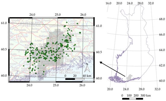
2.1. Study Area and Harvester Data
Preprocessing of Harvester Data
2.2. Reference Stand Data
2.3. The Automated Stand Delineation Method
2.3.1. Algorithm A1: Separation of External Strip Roads
2.3.2. Algorithm A2: Stand Formation
2.3.3. Algorithm A3: Intersecting Stand Polygons
2.4. Method for Validating the Stand Delineations
3. Results
3.1. Robustness of Automated Method and Overall Results of the Dataset
3.2. Results of Estimated GNSS Accuracy
3.3. Comparison of Stands
3.3.1. Ensuring the Similarity of Compared Stands
3.3.2. Comparison Results of Aerial Images and GNSS References
3.3.3. Adjusting the Area Parameter of the Automated Stand Delineation Method
3.3.4. Comparison Results of Harvested Stands and References
4. Discussion
5. Conclusions
Supplementary Materials
Author Contributions
Funding
Acknowledgments
Conflicts of Interest
Appendix A
| Estimation method of GNSS accuracy: |
| Input: harvester location points P of one harvested object Convert the Np input points into line which is ordered by StemNumber. This ordering is based on the cutting order of the trees (see Figure A1). Explode the line geometry into separate line segments. // Measure the total length of the segments which are not too long (some segments can be rather // long due to the cutting order and harvester movements, see Figure A1c). Initialize LGNSS = 0. Loop over line segments s, and exclude segment if it is too long: If L(s) < 20 m: LGNSS = LGNSS + L(s). End if. End loop. A.1. Obtain the average length per total amount of segments: LGNSS = LGNSS/(Np − 1). // Set the GNSS accuracy labels. Initialize quality variable QGNSS = “More accurate”. // Change the label if needed based on the obtained average length LGNSS and the amount of data // points. If (LGNSS > 3.5 m and Np > 120): QGNSS = “Less accurate”. End if. |

Appendix B
| Algorithm A1: Stand clustering and strip road separation |
| Input: harvester location points P of one harvested object Set the parameter values based on the accuracy of GNSS positioning. // Currently, only one parameter is adjusted by the GNSS accuracy: number of points for averaging // Nave. For more accurate GNSS, Nave = 11 and for less accurate GNSS, Nave = 31. // Calculate average locations for all input points. Loop over points pi ϵ P: Request Nave nearest points PN from P with respect to the point pi by spatial query. // Find points which are closer than stand buffer BS = 23 m to pi. Loop over pn ϵ PN: If distance D(pi, pn) > BS: Remove pn from PN. End if. End loop. Obtain averaged coordinates, noted as <pi>, from remaining points pn ϵ PN. End loop. // Make preliminary classification of the points into two categories, stand or strip road leading to // stand. If point has adjacent points as suitable distance, it belongs to stand. See Figure A2. Loop over points <pi> ϵ P: For point <pi>, obtain the closest point <pc> where D(<pi >,<pc>) > 5 m. Determine the bearing of the found point <pc> from the point <pi>. Convert the bearing into scale β ϵ [0°, 180°]. Create sector polygons Gsec perpendicularly to the converted bearing direction β, using sector angle γ = 22°:
Gsec = sector(α, r = 30 m) − sector(α, r = 8 m),
B.1. // Find if the sector polygons intersect with other averaged points. If Gsec intersect with other point locations <pj> ϵ P, j ≠ i: Set index1 = 1 for <pi>. Else: Set index1 = 0 for <pi>. End if. End loop. // Smoothen the classification by averaging the preliminary classification results (see Figure A3a // and Figure A3b.) For that, define strip road buffer value Bsr = 8 m. B.2. Loop over all points <pi> ϵ P: Request points <pa> ϵ PA from P such that D(<pi>, <pa>) < Bsr. Average the values of index1 of points PA: <index1> = Σ(index1)/N(PA). // Study if <index1> for PA exceeds limit value 0.4. If <index1> >= 0.4: Set index2 = 1 for <pi>. Else: Set index2 = 0 for <pi>. End if. End loop. B.3. // Aggregate stand and strip road points into multipoint “motifs” Mk where k denotes the index of // the motif. Each motif relates to either stand points or strip road points, depending on the value // of index2 of the tree points assigned to the motif. Initialize k = 0. Loop over points [<p1>, <pN(P)-1>] ϵ P: If <pi>(index2) == <pi+1>(index2): Switch <pi>(index2): Case 1: Label <pi> to (stand) motif Mk. Case 0: If D(<pi>, <pi+1>) < Bsr: Label <pi> to (strip road) motif Mk. Else: Increase motif index k to k+1. End if. End switch. Else: Increase motif index k to k+1. End if. End loop. // Handle last point <pN(P)> ϵ P. Switch <pN(P)>(index2): Case 1: Label <pN(P)> to (stand) motif Mk. Case 0: Label <pN(P)> to (strip road) motif Mk. End switch. Merge all motifs Mk(index2 == 1) to M∪, and set index3 = 1 for points <p> ∊ M∪. If M∪ has type “multipolygon”, convert it to single polygons. Buffer M∪ and all Mk(index2 == 0) with respective buffer distances BS, Bsr (see Figure A3c). Merge the overlapping mk,B ∊ Mk,B(index2 == 0) to M∪,B and their points (see Figure A3c). // To identify spur trails, limit value of relative area Ar is obtained from geometric considerations // of parameter Lst = 15 m which describes the maximum spur trail length which should be still // merged into the stand (i.e. it is too short for being a strip road leading to stand):
Ar = (π(Bsr)2/2 + 2(BS − Lst)Bsr)/(π(Bsr)2 + 2BsrLst).
Loop over m∪ ∊ M∪: Loop over m∪,B ∊ M∪,B(index2 == 0): If A(m∪ ∩ m∪,B) > Ar: Set index3 = 1 for points <p> ∊ m∪,B. // The strip road motif m∪,B is a spur trail and it is returned into the stand. See //Figure A3c,d. Else: Set index3 = 0 for points <p> ∊ m∪,B. End if. End loop. End loop. Aggregate points P(index2 == 1) again into motifs Mk,upd similarly as in Stage B.3. but using distance condition D(<pi>, <pj>) < BS. Buffer motifs Mk,upd with BS to motifs Mk,upd,B. Merge the points of overlapping mk,upd,B ∊ Mk,upd,B to form groups of stand points PS. Give unique labels StandID for the stand-wise point groups PS. |


Appendix C
| Recognizing the dense strip roads: |
| Input: strip road threes PSR from Algorithm A1 of one harvested object // Calculate average location for the strip road points in similar way as in Algorithm A1 but with // different parameter values. Here a single value for Nave = 15 is used for all strip roads // independently from GNSS accuracy, as the variance in strip road point densities is larger than // in typical stands, especially towards the sparse values, and therefore the role of GNSS accuracy // is not as pronounced. Loop over points pi ϵ PSR: Request Nave nearest points PN from PSR with respect to the point pi by spatial query. // Find points which are closer than strip road distance Dsr = 10 m to pi. Loop over pn ϵ PN: If D(pi, pn) > Dsr: Remove pn from PN. End if. End loop. Average the coordinates of remaining points of PN and store the averaged location for pi. End loop. // Buffer the averaged strip road points. Loop over points pi ϵ PSR: Buffer the averaged coordinates of point pi to geometry gi by buffer width Btemp = Wsr + Dsr/2, where strip road half width Wsr = 2.25 m. End loop. // Merge the buffered point geometries into identifiable strip road parts in the following manner. Merge the overlapping gi into one polygon geometry G∪,sr and the respective points into group of points P∪,sr. Obtain the amount of points Nsr = N(P∪,sr) in each strip road part. // Find those strip road parts that should rather be stands than strip roads leading to stands. // They have high enough removal density of trees per unit area, DA. Loop over strip road parts P∪,sr: Calculate removal density DA = Nsr/A(G∪,sr). // Check the removal density of strip road part. If (DA > 0.05 points/m2 and Nsr >= 15): Give unique StandID for points pi ∊ P∪,sr to label the points as a stand. End if. End loop. |
Appendix D
| Algorithm A2: Stand polygon formation |
| Input: stand points Pstands for one harvested object (including dense strip road points) Find unique values of StandID from Pstands and add them to list Stands. Loop over SI ∊ Stands: Select points of one stand PS = ps ∊ Pstands, ps(StandID) == SI. // Check that the group of stand points PS consists of at least three points at different locations // which are not farther than outlier distance Dmax = 19 m from each other. If (∄ p1, p2, p3 ∊ PS such that pi(xi, yi) ≠ pj(xj, yj) where i, j ∊ [1,3] and D(pi, pj) < Dmax): Stop the geoprocessing here. No resulting stand delineations will be produced for PS. End if. // Remove all duplicate coordinates from the stand points. If pi(xi, yi) = pj(xj, yj), i ≠ j: Remove pi from PS. End if. D.1. // Remove all points which are farther than outlier distance Dmax away from other points. Loop over pi ϵ PS: Request one nearest neighbour pN1 for point pi. // Study how far the point pN1 is from other points. If D(pi, pN1) > Dmax: Remove pi from PS. End if. End loop. Create a Delaunay triangulation T for the remaining points in PS. Define maximum triangle edge value Tmax = 35 m. Set selected triangles Tsel: t ϵ Tsel if edge(t, i) < Tmax and i ∊ [1,3]. Dissolve all selected triangles t ∊ Tsel to geometry GD. Buffer the dissolved polygon geometry GD outwards by value B2 to obtain geometry GD,B. D.2. Check geometry type of GD,B. In case of type “multipolygon”, convert it to single polygons. Add GD,B to list Gobject. End loop. // Obtain stand geometries GS for harvested object by dissolving possibly intersecting stand and // strip road polygons by ObjectID. If gm ∩ gn, m ≠ n and m,n ∊ N(Gobject): Set GD,IS = gm ∩ gn, m ≠ n and m,n ∊ N(Gobject). Add GS,∪ = ∪ GD,IS, g ∊ GD,IS, to stand geometries GS. End if. Loop over g ∊ Gobject for which ∄ (gm ∩ gn, m ≠ n and m,n ∊ N(Gobject)): Add g to stand geometries GS. End loop. D.3. Label the obtained stand delineations GS (harvested stands) uniquely within object by StandID2. Then stand is identified based on ObjectID and the stand label. |
Appendix E
| Algorithm A3: Balancing overlapping stand boundaries |
| Input: a set of stand delineation polygons S to be balanced (note that geometry type “multipolygon” needs to be converted into single polygons) Put the first input stand S1 from input stands S as such into list UpdatedStands. In case of previous stands existing, put only them to the list. Loop over rest of the input stands S0i, i = [2, N(S)]: (if previous stands exist, use i = [1, N(S)]) Initialise IScounter = 0. E.1. Loop over updated stand polygons Su ∊ UpdatedStands: Initialise list DP to store the division points. // Check whether stand polygons intersect. Ensure that if the stand Si had previous // intersections, the latest version of the stand geometry is used. Set Si = S0i. If (IScounter > 0): Set Si = Si,F. End if. // If stand polygons do not intersect, go to next stand polygon. If not Si ꓵ Su: Go to E.1. End if. Convert Si, Su into boundary line geometries Li, Lu. Find the intersections of lines Li, Lu and call them vertex points PV. Add pV ∊ PV into list DP. // See Figure A4a for example of determining the vertex points. Obtain buffered geometries GV by buffering PV with small value. Here 0.4m was used. Take intersection geometry GIS = Si ꓵ Su and ensure that it has geometry type “polygon” (in case of “multipolygon”, convert to single polygons). Select GIS,s = gIS ∊ GIS such that A(gIS) > Amin. E.2. Initialise boolean variable CannotSplit = FALSE. Loop over intersection polygons gIS ∊ GIS,s: // Check how many of the vertex points pV ∊ PV intersect with gIS. If N(pV ꓵ gIS) ≠ 2: Set CannotSplit = TRUE. End if. // Check whether the polygon gIS has holes in its geometry. If holes exist in gIS: Set CannotSplit = TRUE. End if. End loop. E.3. // In case of CannotSplit == TRUE, intersection GIS cannot be split unambiguously. If CannotSplit == TRUE: // It is possible that the stand has been added into the updated stands, if it // had other intersections before the non-splittable intersection, see Stage E.5. // Here non-splittable stands are removed from the resulting stand network. If IScounter > 0: Remove Si* from from list UpdatedStands where Si*(StandID2) == Si(StandID2). End if. Set IScounter = IScounter + 1. Go to E.1. End if. // From here on the cases CannotSplit == FALSE are handled. Start finding the // possible empty slots between the intersecting stand polygons. For that, the stands // cannot have holes i.e. internal rings in their geometries. If Si or Su has holes: Fill the holes and obtain filled stand polygons Si,f and Su,f. End if. Obtain combined geometry S∪ = Si,f ∪ Su,f. // The empty slot polygons that lie between the intersecting stands will appear as // internal rings in S∪. Extract the hole polygons GH from S∪. Select GH,s = gH ∊ GH such that Amin < A(gH) < Amax. Add all polygons of GIS,s and GH,s to Gsplit for splitting. // Form the division line points by geoprocessing the polygon geometries Gsplit. Loop over gsplit ∊ Gsplit: Convert gsplit into its boundary lines Lg. Erase buffered vertices: Lg,E = Lg − GV. Manipulate Lg,E to form two, continuous lines L1 and L2 at opposite sides of the polygon gsplit, between vertex points. Create equal amount Nr sample points for lines L1, L2 at equal fractions of their lengths from one vertex point pV ∊ PV onwards. // Points ri,1, ri,2 ∊ Nr, i ∊ [1, Nr] form counterpart pairs, and their average determines // the location of the division line point. A few tens of points is a recommendable // amount of sample points. Lengths of L1, L2 can be used to adjust the amount of // points. See Figure A4a,b. Loop over i ∊ [1, Nr]: Calculate average <ri> from the coordinates of ri,1, ri,2. If <ri> ꓵ gsplit: Insert <ri> into list DP. End if. End loop. End loop. // Examine division points DP in order to sort them. Take a bounding box of Si and corner points PBB of bounding box. Loop over j ∊ [1,4]: Set loop variable Point1 = PBB,j. Set p ∊ DP into list AvailablePoints. Initialise OrderLength = 0 to measure cumulative distance of ordered DP’s. Loop over n ∊ [0, N(DP)]: Find pc such that distance D(Point1, pc) = min(D(Point1, p)) for p ∊ AvailablePoints. Set Point2 = pc. Add pc into list OrderedPoints. If n > 0: Remove Point1 from AvailablePoints. Set OrderLength = OrderLength + D(Point1, Point2). End if. Set loop variable Point1 = Point2. End loop. Store OrderedPoints and respective values of OrderLength. End loop. Find order index j which has shortest OrderLength. Create division line geometry LD from OrderedPoints of order j. Buffer LD with 0.3 m to obtain geometry GL. Split polygons Gsplit (B.II.14) by division line LD to obtain halved geometries Gdiv. // The split can be done e.g. using polygon-line-intersection tool in GIS. Erase buffered line from halved geometries: Gdiv,E = Gdiv − GL. Buffer polygons Gsplit with 0.1 m to obtain Gsplit,B. Buffer the polygons Gdiv,E with 0.15 m to obtain Gdiv,E,B. Buffer the Gdiv (B.II.20) with 0.4 m to obtain Gdiv,B. Erase intersection from stand polygons: Si,E = Si − Gsplit,B and Su,E = Su − Gsplit,B. E.4. // To obtain a proper new stand boundary (Figure A4d), examine which half of Gdiv // belongs to which stand. This is done by intersecting Si,E and Su,E with Gdiv,E,B. Loop over gdiv,E,B ∊ Gdiv,E,B: If N(Gdiv) == N(Gdiv,E,B): // The following is possible since the ordering of features remains in GIS // program during geoprocessing. If gdiv,E,B ꓵ Si,E: Record that gdiv ∊ Gdiv, gdiv(id) == gdiv,E,B(id) belongs into Si. End if. If gdiv,E,B ꓵ Su,E: Record that gdiv ∊ Gdiv, gdiv(id) == gdiv,E,B(id) belongs into Su. End if. End if. If N(Gdiv) ≠ N(Gdiv,E,B) or (gdiv,E,B ꓵ Si,E and gdiv,E,B ꓵ Su,E): If A(gdiv,E,B ꓵ Si,E) > A(gdiv,E,B ꓵ Su,E): Loop over polygons gdiv ∊ Gdiv: If A(gdiv,E,B ꓵ gdiv) > 0.3 * A(gdiv,E,B): Record that gdiv belongs into Si. End if. End loop. End if. If A(gdiv,E,B ꓵ Si,E) < A(gdiv,E,B ꓵ Su,E): Loop over polygons gdiv ∊ Gdiv: If A(gdiv,E,B ꓵ gdiv) > 0.3 * A(gdiv,E,B): Record that gdiv belongs into Su. End if. End loop. End if. End if. End loop. Select small polygons Gm = g ∊ {GIS, GH} such that A(g) < Amin. // Handle gm ∊ Gm in alternating manner without splitting as A(gm) << A(typical // stand). Loop over l ∊ [0, N(Gm)]: If l is even number: Record that gm ∊ Gm belongs to Si. Else: Record that gm ∊ Gm belongs to Su. End if. End loop. List the halved and small polygons: GF = Gdiv + Gm. // To obtain the resulting stand polygons with proper stand boundaries, erase gF ∊ GF // from the stands based on recorded information to which stand, Si or Su, they // belong. Obtain Si,F = Si − gF where gF ∊ GF and gF ∊ Su. Obtain Su,F = Su − gF where gF ∊ GF and gF ∊ Si. Change geometry Su → Su,F in UpdatedStands. E.5. // Store the resulting geometry of Si,F depending on whether this was its first // intersection with stands in UpdatedStands. If IScounter == 0: Add Si,F into list UpdatedStands as a new entry. Else: Find stand Si* from list UpdatedStands where Si*(StandID2) == Si(StandID2) (it should be the latest entry of the list). Change geometry Si* → Si,F. End if. Set IScounter = IScounter + 1. End loop. // Check if the stand did not have intersections with updated stands. If IScounter == 0: Add Si as such into list UpdatedStands. End if. End loop. The list UpdatedStands contains now all the stands for which the balanced delineation could be formed. Those stands which cannot be split in this way with the previously updated stands, can be separated from Stage E.3. |

Appendix F

Appendix G
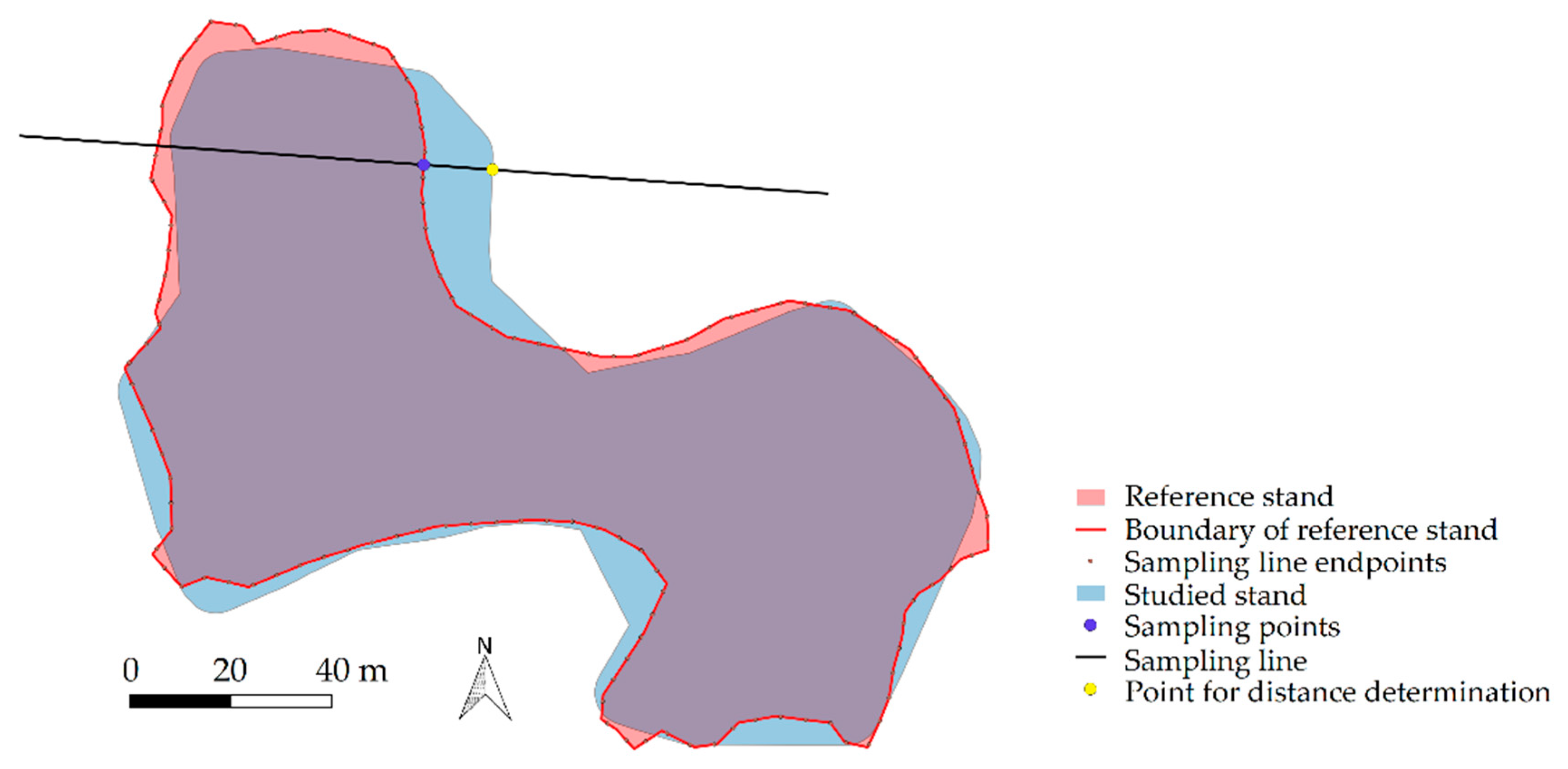
| Determining perpendicular distances between stand boundaries: |
| Input: two stand polygons S and SR without inner rings Convert the compared two stand polygons into boundary line geometries. Denote boundary of stand polygon S by L0 and boundary of the reference polygon SR by LB. // Sample the stand boundary of reference stand. Obtain the length of LB. Calculate amount of samples as NSB = int(LB/Lsegm) where Lsegm = 5m. Split LB into lines LS of length Lsegm. // The split can be started e.g. from the point which appears first in the list of boundary // coordinates of polygon’s presentation in GIS. One segment shorter than Lsegm typically occurs // at the “end” of the boundary line. // Find the perpendicular distance values. Initialize lists Distances and NormalAngles. Loop over lS ∊ LS: Approximate lS by a segment s between the start point lS,1 and end point lS,2 of the line lS. Obtain bearing βS of lS,2 from lS,1. Obtain normal angle αN = βS − 90°. If needed, convert αN ∊ [0°, 360°]. Insert αN into list NormalAngles. Obtain center point sc of s. Create normal lines perpendicular to s with help of αN. The lines are at both sides of the stand boundary: LN,1 outwards (angle αN) and LN,2 inwards (angle αN + 180°) of the stand and have adequate length each (e.g. 80 m). // Determine the distance value at sc. Make agreement of positive and negative direction // with respect to the progress of stand boundary coordinates list. Find the possible intersection point(s) P1 = LN,1 ∩ L0. If N(P1) > 0: Take point p1 which has min(D(p1, sc)), p1 ∊ P1. Measure d = D(p1, sc) and give it positive sign. Add d into list Distances. End if. Find the possible intersection point(s) P2 = LN,2 ∩ L0. If N(P2) > 0: Take point p2 which has min(D(p2, sc)), p2 ∊ P2. Measure d = D(p1, sc) and give it negative sign. Add d into list Distances. End if. End loop. // Pick the distance values for different normal angles covering the main directions. This is done // to find out if the compared stand has shifted with respect to the reference stand. Initialize separate distance lists for all eight main directions. Loop over NormalAngles: Loop over main directions (N, NW, E, SE, S, SW, W, NW): Denote bearing of main direction as γ (e.g. γSE = 135°), and if needed, convert all angle values to [0°, 360°]. If αN in [γ − 45°, γ + 45°]: Insert Distances[index(αN)] into the relevant list of main direction distances. End if. End loop. End loop. Calculate mean and standard deviation of all distances. Calculate means of distances at main directions. Calculate the net shifts at four directions N−S, NE−SW, E−W and SE−NW by subtracting the respective mean values in those directions. |
References
- Holopainen, M.; Vastaranta, M.; Hyyppä, J. Outlook for the next generation’s precision forestry in Finland. Forests 2014, 5, 1682–1694. [Google Scholar] [CrossRef] [Green Version]
- Siipilehto, J.; Lindeman, H.; Vastaranta, M.; Yu, X.; Uusitalo, J. Reliability of the predicted stand structure for clear-cut stands using optional methods: Airborne laser scanning-based methods, smartphone-based forest inventory application Trestima and pre-harvest measurement tool EMO. Silva Fenn. 2016, 50, 1568. [Google Scholar] [CrossRef] [Green Version]
- Malinen, J.; Kilpeläinen, H.; Ylisirniö, K. Description and evaluation of Prehas software for preharvest assessment of timber assortments. Int. J. For. Eng. 2014, 25, 66–74. [Google Scholar] [CrossRef]
- Davis, L.S.; Johnson, K.N. Forest Management, 3rd ed.; McGraw-Hill Book Company: New York, NY, USA, 1987. [Google Scholar]
- Poso, S. Kuviottaisen arvioimismenetelmän perusteita. [Basic features of forest inventory by compartments]. Silva Fenn. 1983, 17, 313–349. [Google Scholar] [CrossRef] [Green Version]
- Leckie, D.G.; Gougeon, F.A.; Walsworth, N.; Paradine, D. Stand delineation and composition estimation using semi-automated individual tree crown analysis. Remote Sens. Environ. 2003, 85, 355–369. [Google Scholar] [CrossRef]
- Radoux, J.; Defourny, P. A quantitative assessment of boundaries in automated forest stand delineation using very high resolution imagery. Remote Sens. Environ. 2007, 110, 468–475. [Google Scholar] [CrossRef]
- Næsset, E.; Gobakken, T.; Holmgren, J.; Hyyppä, H.; Hyyppä, J.; Maltamo, M.; Nilsson, M.; Olsson, H.; Persson, Å.; Söderman, U. Laser scanning of forest resources: The Nordic experience. Scand. J. For. Res. 2004, 19, 482–499. [Google Scholar] [CrossRef]
- Maltamo, M.; Eerikäinen, K.; Packalén, P.; Hyyppä, J. Estimation of stem volume using laser scanning-based canopy height metrics. Forestry 2006, 79, 217–229. [Google Scholar] [CrossRef] [Green Version]
- Holopainen, M.; Vastaranta, M.; Rasinmäki, J.; Kalliovirta, J.; Mäkinen, A.; Haapanen, R.; Melkas, T.; Yu, X.; Hyyppä, J. Uncertainty in timber assortment estimates predicted from forest inventory data. Eur. J. For. Res. 2010, 129, 1131–1142. [Google Scholar] [CrossRef]
- Næsset, E. Predicting forest stand characteristics with airborne scanning laser using a practical two-stage procedure and field data. Remote Sens. Environ. 2002, 80, 88–99. [Google Scholar] [CrossRef]
- White, J.C.; Wulder, M.A.; Varhola, A.; Vastaranta, M.; Coops, N.C.; Cook, B.D.; Pitt, D.; Woods, M. A best practices guide for generating forest inventory attributes from airborne laser scanning data using an area-based approach. For. Chron. 2013, 89, 722–723. [Google Scholar] [CrossRef] [Green Version]
- Valonen, M.; Haltia, E.; Horne, P.; Maidell, M.; Pynnönen, S.; Sajeva, M.; Stenman, V.; Raivio, K.; Iittainen, V.; Greis, K.; et al. Finland’s Model in Utilising Forest Data. PTT Reports 261. Pellervo Economic Research PTT. 2019. Available online: https://www.metsakeskus.fi/sites/default/files/ptt-report-261-finlands-model-in-utilising-forest-data.pdf (accessed on 23 June 2020).
- Rasinmäki, J. Management of Multi-Scale Forest Resource Data over Time. Dissertationes Forestales 49. Ph.D. Thesis, Department of Forest Resource Management, Faculty of Agriculture and Forestry, University of Helsinki, Helsinki, Finland, 2007. Available online: http://www.metla.fi/dissertationes/df49.htm (accessed on 23 June 2020).
- Saukkola, A.; Melkas, T.; Riekki, K.; Sirparanta, S.; Peuhkurinen, J.; Holopainen, M.; Hyyppä, J.; Vastaranta, M. Predicting Forest Inventory Attributes Using Airborne Laser Scanning, Aerial Imagery, and Harvester Data. Remote Sens. 2019, 11, 797. [Google Scholar] [CrossRef] [Green Version]
- Lindroos, O.; Ringdahl, O.; La Hera, P.; Hohnloser, P.; Hellström, T. Estimating the Position of the Harvester Head-a Key Step towards the Precision Forestry of the Future? Croat. J. For. Eng. 2015, 36, 147–164. [Google Scholar]
- StanForD/StanForD 2010-Standard for Forest Machine Data and Communication. Skogforsk, Sweden, 2020. Available online: http://www.skogforsk.se/english/projects/stanford/ (accessed on 15 June 2020).
- Bhuiyan, N.; Möller, J.J.; Hannrup, B.; Arlinger, J. Automatisk Gallringsuppföljning-Areal Beräkning Samt Registrering av Kranvinkel för Identifiering av Stickvägsträd och Beräkning av Gallringskvot. [Automatic Follow-up of Thinning-Stand Area Estimation and Use of Crane angle Data to Identify Strip Road Trees and Calculate Thinning Quotient.] Arbetsrapport 899–2016. Skogforsk, Sweden, 2016. In Swedish with Abstract in English. Available online: https://www.skogforsk.se/cd_20190114161523/contentassets/6eda4307138347648171f87e3d9a3885/automatisk-gallringsuppfoljning-arealberakning-samt-registrering-av-kranvinkel-for-identifiering-av-sticktrad-och-berakning-av-gallringskvot-arbetsrapport-899-2016.pdf (accessed on 23 June 2020).
- Ester, M.; Kriegel, H.-P.; Sander, J.; Xu, X. A Density-Based Algorithm for Discovering Clusters in Large Spatial Databases with Noise. In Proceedings of the 2nd International Conference on Knowledge Discovery and Data Mining (KDD-96), Portland, OR, USA, 2–4 August 1996; AAAI Press: Paolo Alto, CA, USA, 1996; pp. 226–231. [Google Scholar]
- Duckham, M.; Kulik, L.; Worboys, M.; Galton, A. Efficient generation of simple polygons for characterizing the shape of a set of points in the plane. Pattern Recognit. 2008, 41, 3224–3236. [Google Scholar] [CrossRef]
- Yu, X.; Hyyppä, J.; Karjalainen, M.; Nurminen, K.; Karila, K.; Vastaranta, M.; Kankare, V.; Kaartinen, H.; Holopainen, M.; Honkavaara, E.; et al. Comparison of Laser and Stereo Optical, SAR and InSAR Point Clouds from Air- and Space-Borne Sources in the Retrieval of Forest Inventory Attributes. Remote Sens. 2015, 7, 15933–15954. [Google Scholar] [CrossRef] [Green Version]
- Wallenius, T.; Laamanen, R.; Peuhkurinen, J.; Mehtätalo, L.; Kangas, A. Analysing the agreement between an airborne laser scanning based forest inventory and a control inventory—A case study in the state owned forests in Finland. Silva Fenn. 2012, 46, 111–129. [Google Scholar] [CrossRef] [Green Version]
- Laasasenaho, J. Taper Curve and Volume Functions for Pine, Spruce and Birch. Ph.D. Thesis, Communicationes Instituti Forestalis Fenniae, University of Helsinki, Helsinki, Finland, 1982. [Google Scholar]
- Maanmittauksen Ortokuva. [Description of Orthoimages by National Land Survey of Finland]. In Finnish. Available online: https://www.maanmittauslaitos.fi/kartat-ja-paikkatieto/asiantuntevalle-kayttajalle/tuotekuvaukset/ortokuva (accessed on 23 July 2020).
- Äijälä, O.; Koistinen, A.; Sved, J.; Vanhatalo, K.; Väisänen, P. (Eds.) Metsänhoidon Suositukset. [Best Practices for Sustainable Forest Management.] Tapion Julkaisuja. Tapio Oy 2019 In Finnish. Available online: https://www.metsanhoitosuositukset.fi/wp-content/uploads/2019/09/Metsanhoidon_suositukset_Tapio2019_verkko_1.2.pdf (accessed on 24 June 2020).
- Næset, E. Effects of Delineation Errors in Forest Stand Boundaries on Estimated Area and Timber Volumes. Scand. J. For. Res. 1999, 14, 558–566. [Google Scholar] [CrossRef]
- Hyppänen, H.; Pasanen, K.; Saramäki, J. Päätehakkuiden kuviorajojen päivitystarkkuus. [Accuracy of updating stand boundaries at final fellings]. Folia For.—Metsätieteen Aikakauskirja 1996, 4, 321–335. [Google Scholar] [CrossRef]
- Courteau, J.; Darche, M.-H. A Comparison of Seven GPS Units under Forest Conditions; Special report 120; Forest Engineering Research Institute of Canada: Vancouver, BC, Canada, 1997. [Google Scholar]
- Darche, M.-H. A Comparison of Four New GPS Systems under Forest Conditions; Special report 128; Forest Engineering Research Institute of Canada: Vancouver, BC, Canada, 1998. [Google Scholar]
- Næsset, E. Effects of differential single- and dual-frequency GPS and GLONASS observations on point accuracy under forest canopies. Photogramm. Eng. Remote Sens. 2001, 67, 1021–1026. [Google Scholar]
- Meneguzzo, D.M.; Liknes, G.C.; Nelson, M.D. Mapping trees outside forests using high-resolution aerial imagery: A comparison of pixel- and object-based classification approaches. Environ. Monit. Assess. 2013, 185, 6261–6275. [Google Scholar] [CrossRef]
- Gasparovic, M.; Dobrinic, D.; Medak, D. Geometric accuracy improvement of WorldView-2 imagery using freely available DEM data. Photogramm. Rec. 2019, 34, 266–281. [Google Scholar] [CrossRef]
- Hughes, M.L.; McDowell, P.F.; Marcus, W.A. Accuracy assessment of georectified aerial photographs: Implications for measuring lateral channel movement in a GIS. Geomorphology 2006, 74, 1–16. [Google Scholar] [CrossRef]
- Topographic Database, National Land Survey of Finland. Available online: https://www.maanmittauslaitos.fi/en/maps-and-spatial-data/expert-users/product-descriptions/topographic-database (accessed on 23 July 2020).
- Valbuena, R.; Mauro, F.; Rodriguez-Solano, R.; Manzanera, J.A. Accuracy and precision of GPS receivers under forest canopies in a mountainous environment. Span. J. Agric. Res. 2010, 8, 1047–1057. [Google Scholar] [CrossRef]
- Ordóñez Galán, C.; Rodríguez-Pérez, J.; Martínez, J.; Garcia Nieto, P.J. Analysis of the influence of forest environments on the accuracy of GPS measurements by using genetic algorithms. Math. Comput. Model. 2011, 54, 1829–1834. [Google Scholar] [CrossRef]


| Harvesting Type (Nstand) | Proportion of Tree Species: Pine/Spruce/Birch/Other, % | A, ha | Ntree per ha | DgM, cm | HgM, m | G, m2/ha | V, m3/ha | |
|---|---|---|---|---|---|---|---|---|
| First thinning (33) | 28/26/41/5 | min | 0.5 | 380 | 11.8 | 11.6 | 3.6 | 26.1 |
| max | 7.9 | 1020 | 27.1 | 20.0 | 13.8 | 123.8 | ||
| mean | 1.9 | 680 | 15.3 | 14.9 | 8.9 | 67.4 | ||
| SD | 1.6 | 180 | 3.0 | 1.8 | 2.8 | 25.6 | ||
| Later thinning (108) | 25/52/19/4 | min | 0.5 | 160 | 13.7 | 13.2 | 5.1 | 49.0 |
| max | 11.8 | 950 | 33.9 | 23.5 | 26.6 | 286.5 | ||
| mean | 2.8 | 530 | 20.5 | 18.2 | 11.2 | 103.5 | ||
| SD | 2.3 | 200 | 4.2 | 2.4 | 4.1 | 46.3 | ||
| Clear cutting (216) | 11/74/12/3 | min | 0.5 | 220 | 14.9 | 15.8 | 8.2 | 65.8 |
| max | 12.4 | 1130 | 46.8 | 29.6 | 41.9 | 562.8 | ||
| mean | 2.4 | 600 | 28.6 | 22.7 | 25.4 | 281.5 | ||
| SD | 1.9 | 180 | 4.4 | 2.4 | 5.4 | 75.0 | ||
| Seed tree or shelter tree cutting (43) | 23/63/11/4 | min | 0.5 | 90 | 16.7 | 14.6 | 2.9 | 30.1 |
| max | 7.2 | 1200 | 39.3 | 27.7 | 34.5 | 423.7 | ||
| mean | 2.0 | 460 | 28.7 | 22.4 | 19.5 | 214.6 | ||
| SD | 1.5 | 190 | 4.9 | 3.0 | 6.7 | 87.0 | ||
| Hold-over cutting 1 (19) | 34/27/34/5 | min | 0.8 | 40 | 23.0 | 20.3 | 2.6 | 29.0 |
| max | 7.9 | 540 | 37.1 | 28.0 | 19.9 | 198.3 | ||
| mean | 2.3 | 190 | 31.0 | 23.8 | 9.0 | 96.8 | ||
| SD | 1.8 | 150 | 4.3 | 2.1 | 5.0 | 51.5 |
| Dataset | N | Area, ha | |||
|---|---|---|---|---|---|
| Min | Max | Mean | SD | ||
| Operative stands | 581 | 0.02 | 12.01 | 1.73 | 1.88 |
| Dense strip road polygons | 206 | 0.01 | 1.00 | 0.13 | 0.11 |
| Oper. stand ∪ dense strip roads | 653 | 0.01 | 12.01 | 1.58 | 1.89 |
| Objects without dense strip roads | 399 | 0.03 | 19.47 | 2.52 | 2.46 |
| Objects with dense strip roads | 413 | 0.02 | 19.56 | 2.49 | 2.48 |
| Harvester ID | Accuracy Label from Known Properties | Numerically Estimated More Accurate GNSS, All Harvesting Types (%) | Numerically Estimated More Accurate GNSS, Thinnings | Numerically Estimated Less Accurate GNSS, All Harvesting Types (%) | Numerically Estimated Less Accurate GNSS, Thinnings | Total Number of Objects |
|---|---|---|---|---|---|---|
| 1 | more accurate | 53 (96) | 10 | 2 (4) | 2 | 55 |
| 2 | more accurate | 105 (92) | 42 | 9 (8) | 3 | 114 |
| 3 | more accurate | 103 (98) | 48 | 2 (2) | 0 | 105 |
| 4 | less accurate | 13 (34) | 0 | 25 (66) | 0 | 38 |
| 5 | less accurate | 19 (45) | 12 | 23 (55) | 14 | 42 |
| 6 | less accurate | 47 (61) | 8 | 30 (39) | 16 | 77 |
| sum | 340 | 120 | 91 | 35 | 431 |
| Area Category, ha | N | Area (AI) | Area (GNSS) | Area (AI ∪ GNSS) | Relative Area | Relative Perimeter | Average PD | RMSE PD |
|---|---|---|---|---|---|---|---|---|
| <0.75 | 3 | 0.23 (0.03) | 0.21 (0.05) | 0.25 (0.04) | 1.13 (0.22) | 1.06 (0.14) | 1.51 (2.57) | 4.80 (3.44) |
| 0.75–1.5 | 5 | 1.10 (0.13) | 1.02 (0.16) | 1.14 (0.14) | 1.09 (0.07) | 0.99 (0.06) | 1.68 (1.62) | 4.75 (2.01) |
| 1.5–3.0 | 4 | 1.87 (0.31) | 1.77 (0.29) | 1.92 (0.31) | 1.06 (0.03) | 0.97 (0.03) | 1.44 (0.49) | 4.73 (1.45) |
| >3.0 | 1 | 5.28 1 | 5.19 1 | 5.44 1 | 1.02 1 | 0.96 1 | 0.68 1 | 5.81 1 |
| Stand Pair | # of Stands | <0.75 ha | 0.75–1.5 ha | 1.5–3.0 ha | >3.0 ha |
|---|---|---|---|---|---|
| AHS vs. GNSS | 27 (26/1) | 7 (7/-) | 11 (11/-) | 8 (7/1) | 1 (1/-) |
| AHS vs. AI | 42 (39/3) | 7 (7/-) | 10 (10/-) | 13 (10/3) | 12 (12/-) |
| Variable | Stand Pair | <0.75 ha | 0.75–1.5 ha | 1.5–3.0 ha | >3.0 ha |
|---|---|---|---|---|---|
| Relative area | AI vs. GNSS | 1.13 (0.22) | 1.09 (0.07) | 1.06 (0.03) | 1.02 (-) |
| AHS vs. GNSS | 1.00 (0.19) | 1.00 (0.08) | 1.07 (0.12) | 1.03 (-) | |
| more accurate | 1.00 (0.19) | 1.00 (0.08) | 1.03 (0.06) | 1.03 (-) | |
| less accurate | - | - | 1.36 (-) | - | |
| AHS vs. AI | 1.16 (0.24) | 0.98 (0.08) | 1.01 (0.05) | 1.00 (0.02) | |
| more accurate | 1.16 (0.24) | 0.98 (0.08) | 1.01 (0.06) | 1.00 (0.02) | |
| less accurate | - | - | 1.00 1 (0.03) | - | |
| Perpendicular distance, m | AI vs. GNSS | 1.5 (2.6) | 1.7 (1.6) | 1.4 (0.5) | 0.7 (-) |
| AHS vs. GNSS | −0.6 (2.5) | −0.3 (2.2) | 2.7 (3.6) | 2.8 (-) | |
| more accurate | −0.6 (2.5) | −0.3 (2.2) | 1.7 (2.8) | 2.8 (-) | |
| less accurate | - | - | 9.2 (-) | - | |
| AHS vs. AI | 1.8 (2.9) | −0.7 (2.0) | 0.35 (2.4) | 0.4 (1.5) | |
| more accurate | 1.8 (2.9) | −0.7 (2.0) | 0.6 (2.6) | 0.4 (1.5) | |
| less accurate | - | - | −0.6 1 (1.2) | - |
© 2020 by the authors. Licensee MDPI, Basel, Switzerland. This article is an open access article distributed under the terms and conditions of the Creative Commons Attribution (CC BY) license (http://creativecommons.org/licenses/by/4.0/).
Share and Cite
Melkas, T.; Riekki, K.; Sorsa, J.-A. Automated Method for Delineating Harvested Stands Based on Harvester Location Data. Remote Sens. 2020, 12, 2754. https://doi.org/10.3390/rs12172754
Melkas T, Riekki K, Sorsa J-A. Automated Method for Delineating Harvested Stands Based on Harvester Location Data. Remote Sensing. 2020; 12(17):2754. https://doi.org/10.3390/rs12172754
Chicago/Turabian StyleMelkas, Timo, Kirsi Riekki, and Juha-Antti Sorsa. 2020. "Automated Method for Delineating Harvested Stands Based on Harvester Location Data" Remote Sensing 12, no. 17: 2754. https://doi.org/10.3390/rs12172754
APA StyleMelkas, T., Riekki, K., & Sorsa, J.-A. (2020). Automated Method for Delineating Harvested Stands Based on Harvester Location Data. Remote Sensing, 12(17), 2754. https://doi.org/10.3390/rs12172754