Diffuse Attenuation of Clear Water Tropical Reservoir: A Remote Sensing Semi-Analytical Approach


 , , , and
Abstract
:
1. Introduction
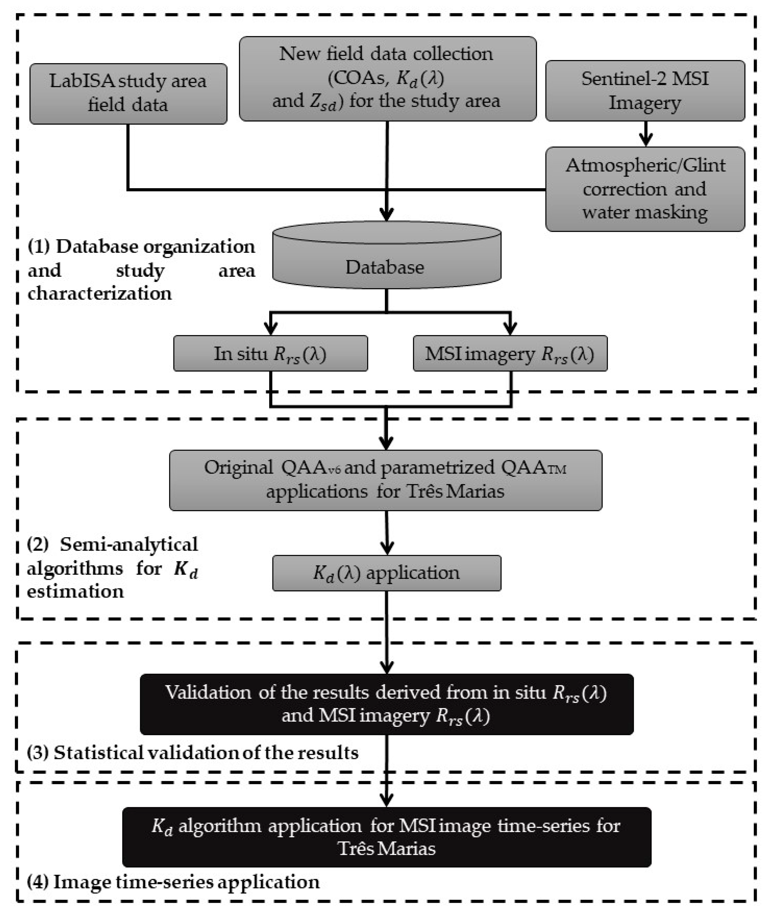
2. Materials and Methods
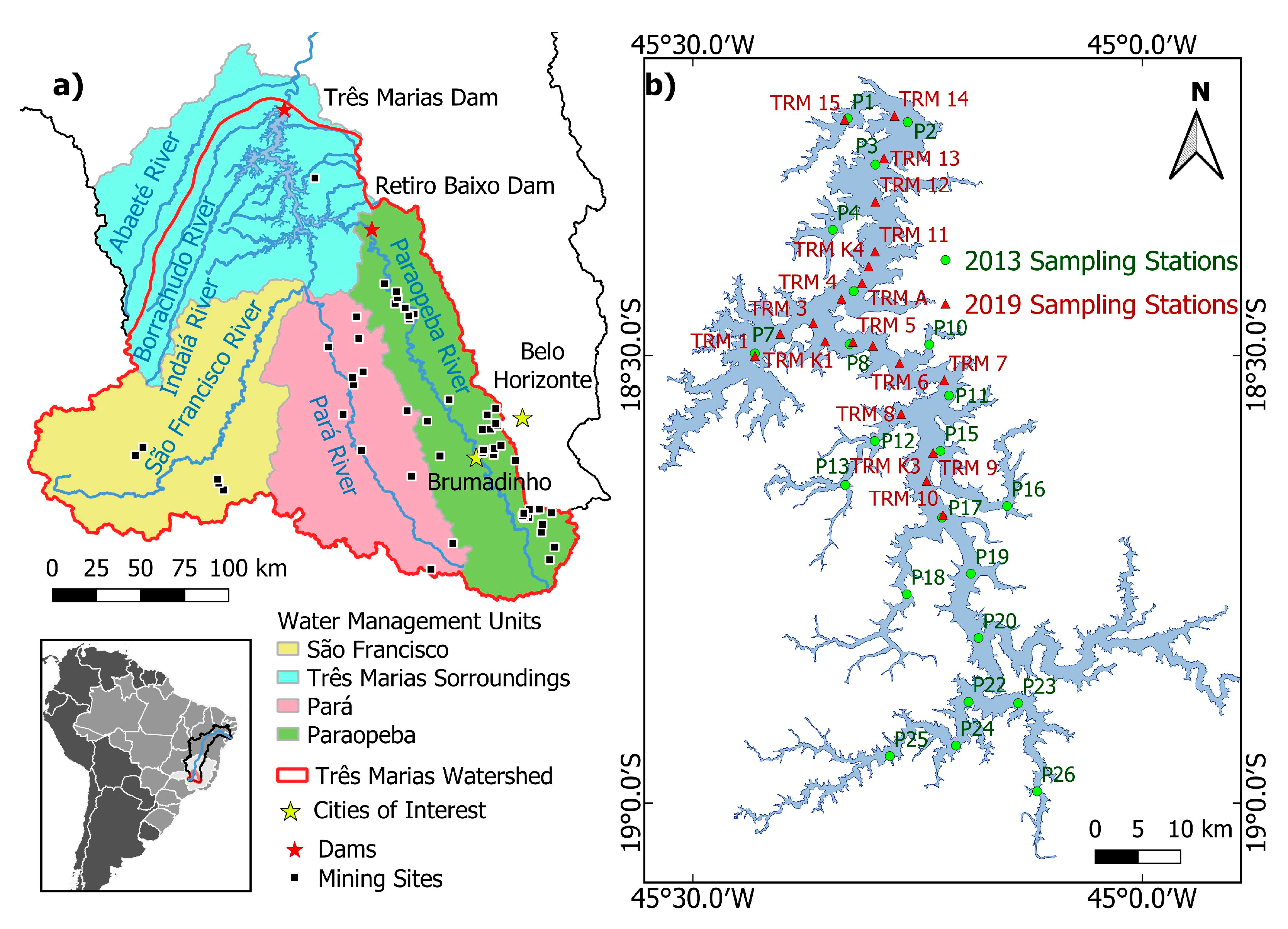
2.1. Study Area
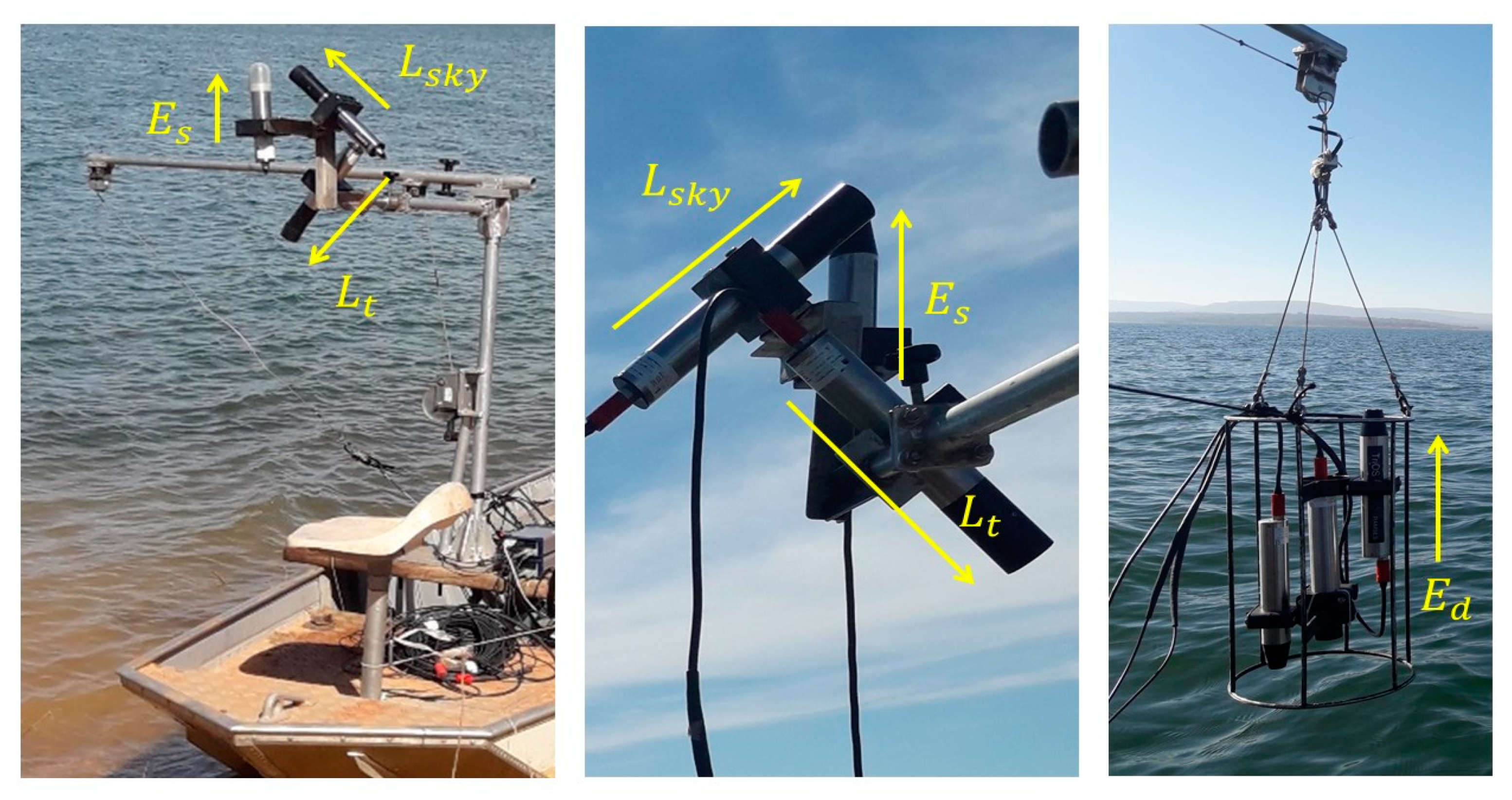
2.2. Field Data Acquisition
2.3. Spectral and Water Quality Field Data
2.3.1. Optically Active Constituents
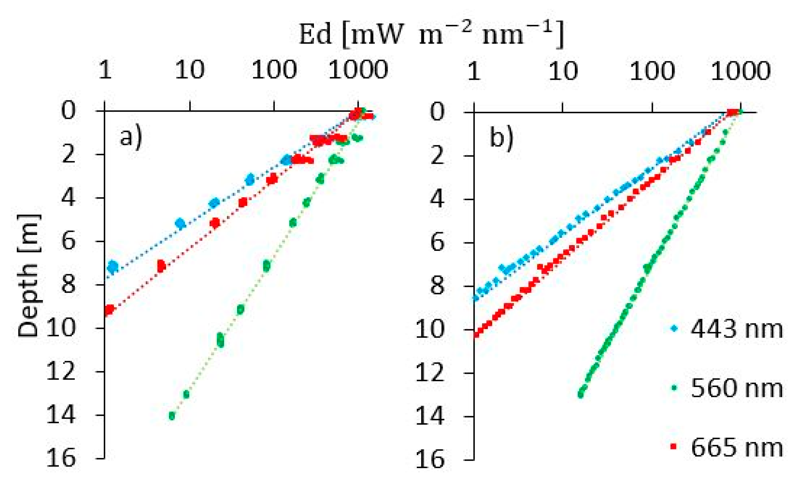
2.3.2. Apparent Optical Properties
2.3.3. Inherent Optical Properties
2.4. Sentinel-2 MSI Data
2.5. Kd(λ) Semi-Analytical Algorithm
2.5.1. Deriving Inherent Optical Properties from Remote Sensing Reflectance
2.5.2. Semi-Analytical Algorithm Validation
2.6. Data Analysis and Accuracy Assessment
2.7. Time Series Kd Algorithm Application
2.7.1. Sentinel-2 MSI Time Series Preprocessing
3. Results
3.1. In Situ Limnology Data
3.2. In Situ Radiometric Characterization
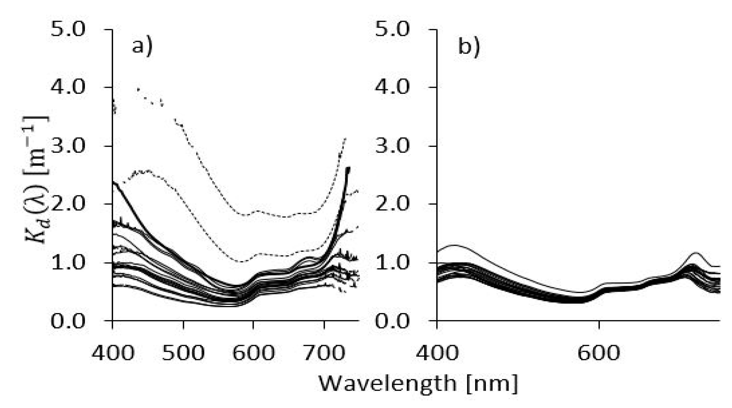
3.2.1. Apparent Optical Properties
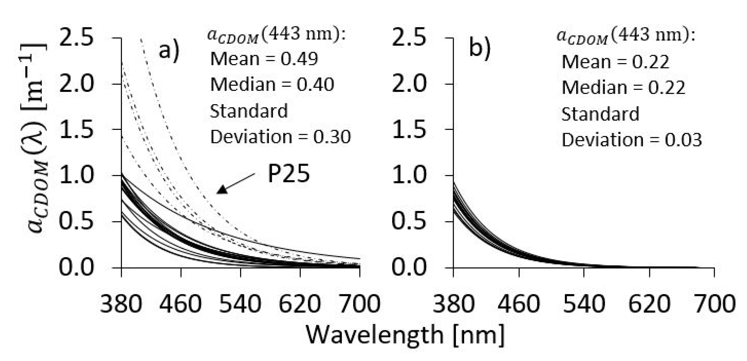
3.2.2. Inherent Optical Properties
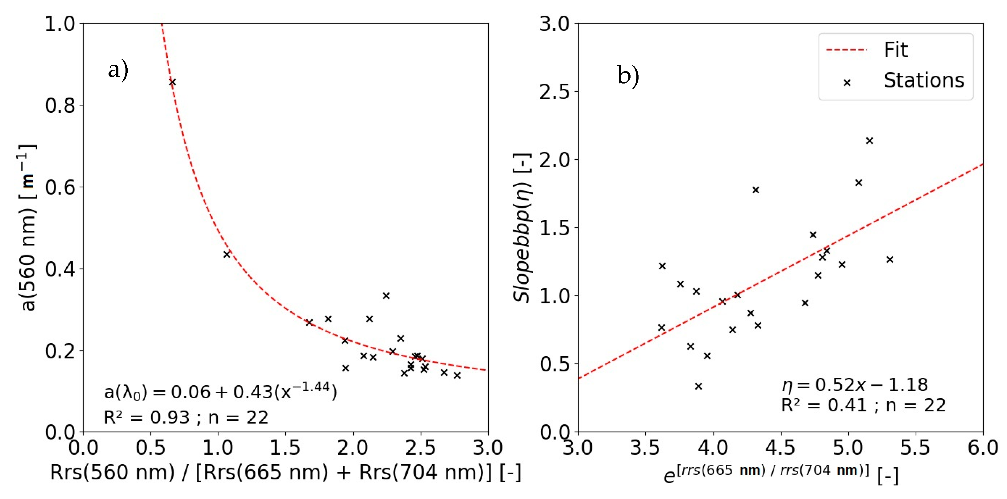
3.3. QAATM Parametrization
3.4. In Situ Validation
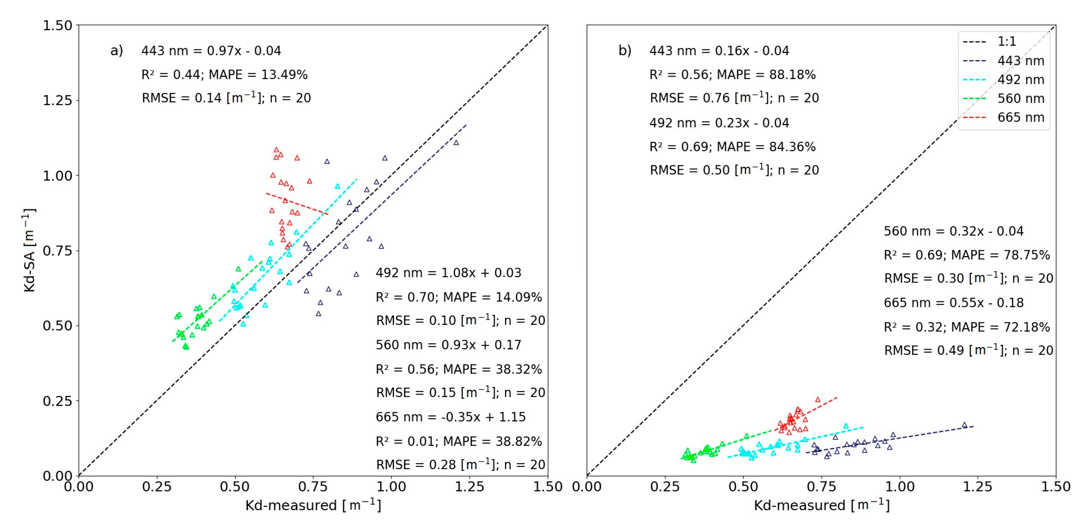
3.5. Satellite Validation
3.5.1. Glint Correction
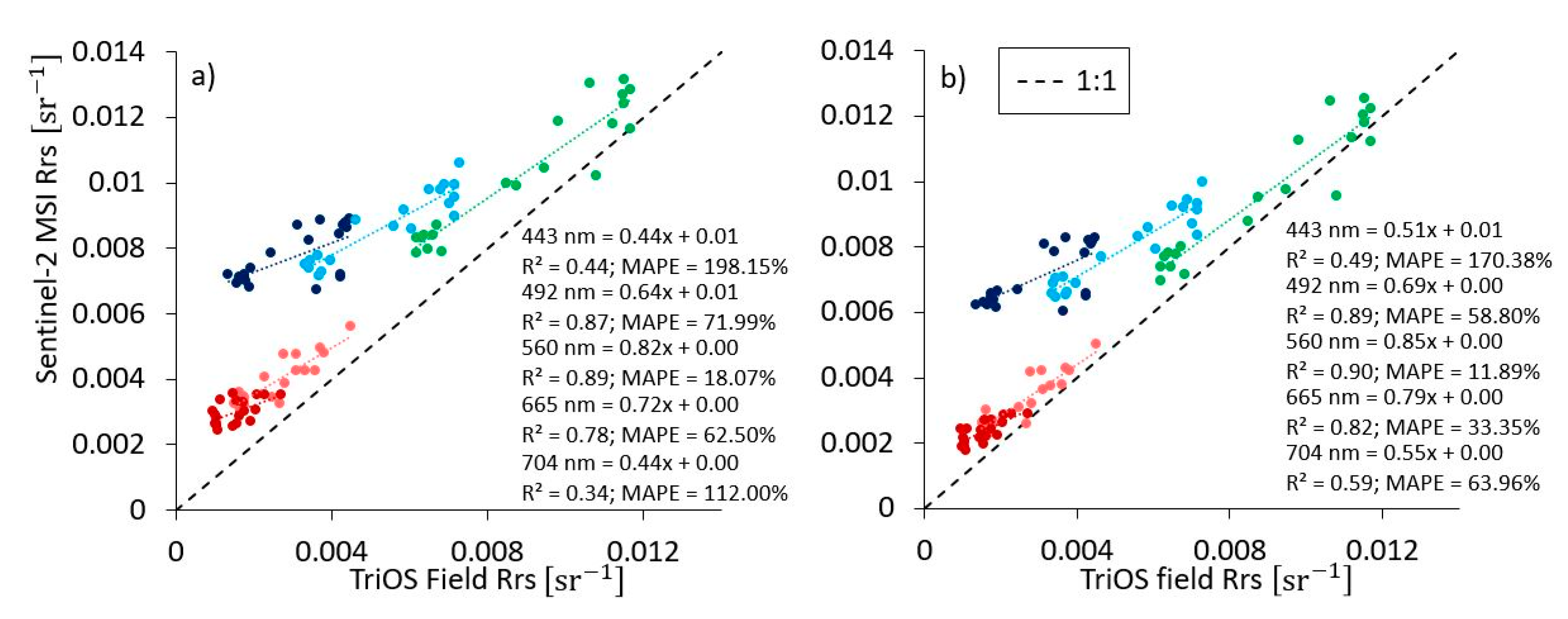
3.5.2. Sentinel-2 MSI Validation
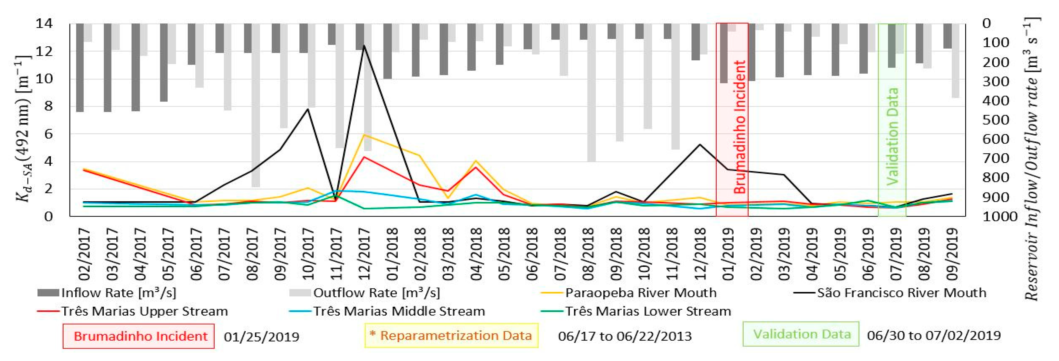
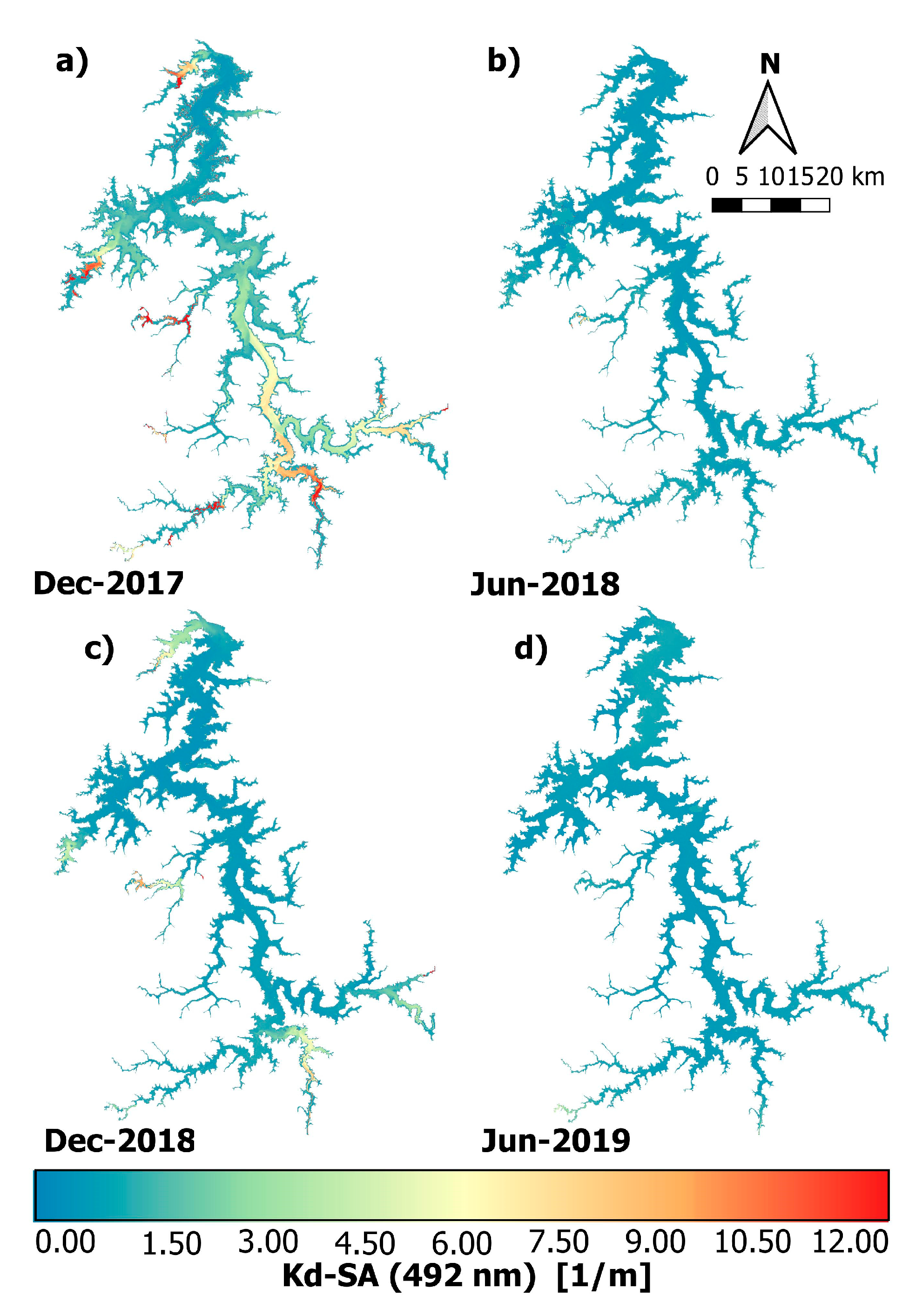
3.5.3. Sentinel -2 MSI Time-Series
4. Discussion
4.1. Algorithms Results Comparison
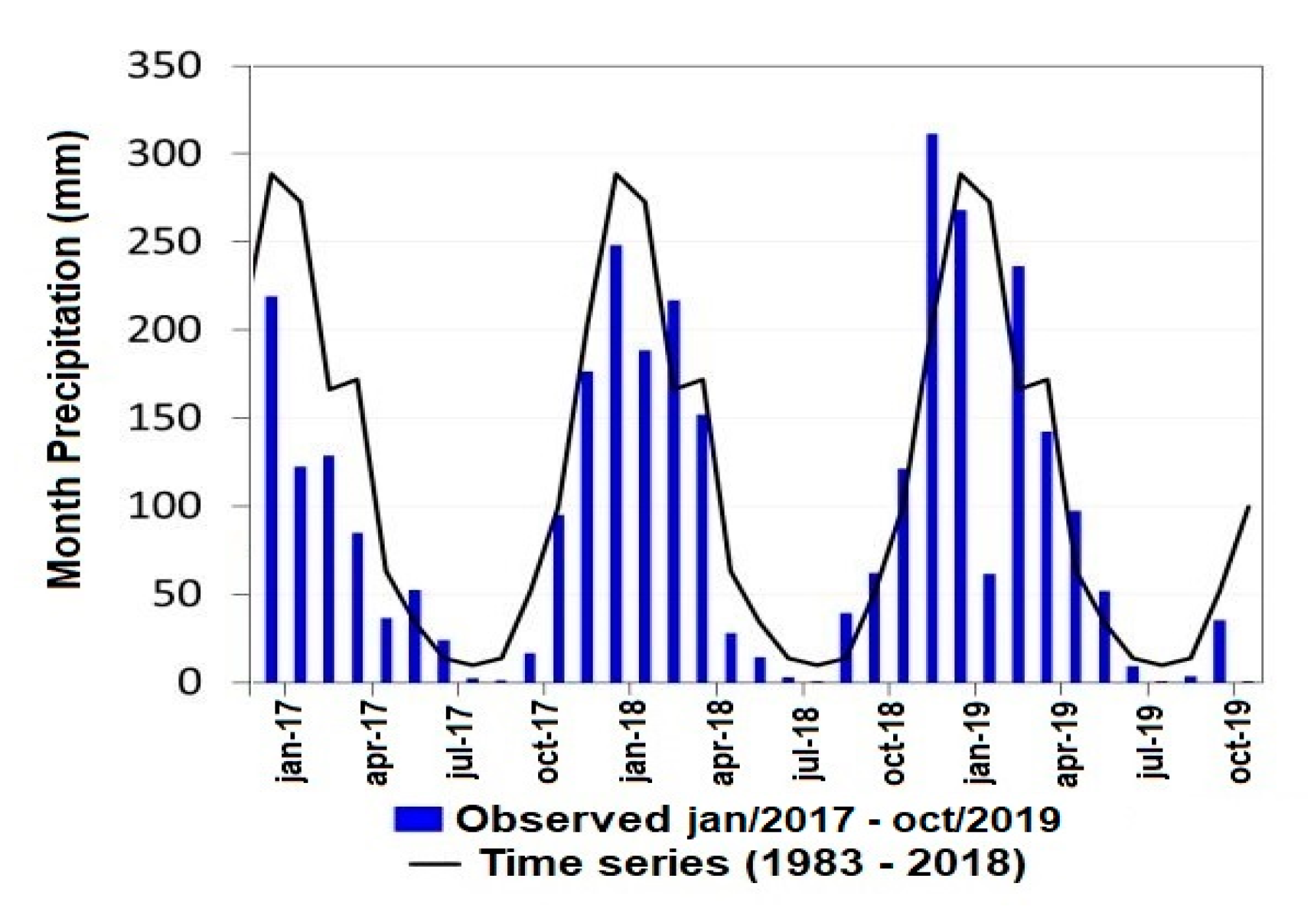
4.2. Temporal Variation of the Diffuse Attenuation Coefficient of the Downwelling Irradiance
4.3. Limitation Factors in the Diffuse Attenuation Coefficient of the Downwelling Irradiance Retrieval
4.3.1. Limitations of the Algorithms
4.3.2. Semi-Analytical Algorithm Reparametrization
5. Conclusions
- Bio optical data collection during rainy periods of the year to reparametrize the algorithm with more variated data;
- Establishment of new algorithms for the correlation between OACs and optical properties of the water to better understand the primary production dynamics of the reservoir;
- Assessment of other atmospheric correction and glint removal methodologies;
- Apply the plus QAATM approach to a time-series including 2020 rainy period to better understand the Brumadinho disaster effects;
- Apply the plus QAATM approach to other small reservoirs just upstream of TM in the Paraopeba River course, assessing the possibility of the retention of sediments coming from Brumadinho into these reservoirs.
Supplementary Materials
Author Contributions
Funding
Acknowledgments
Conflicts of Interest
References
- ANA. Brazilian Water Management Units. Available online: https://metadados.ana.gov.br/geonetwork/srv/pt/main.home (accessed on 27 January 2020).
- ANA. Hydrographic Regions of Brazil. Available online: https://metadados.ana.gov.br/geonetwork/srv/pt/main.home (accessed on 27 January 2020).
- CEMIG. Website CEMIG. Available online: https://www.cemig.com.br/pt-br/a_cemig/Nossa_Historia/Paginas/Usina-Tres-Marias.aspx (accessed on 2 June 2020).
- Tundisi, J.G.; Matsumura-Tundisi, T. Integration of research and management in optimizing multiple uses of reservoirs: The experience in South America and Brazilian case studies. Hydrobiologia 2003, 500, 231–242. [Google Scholar] [CrossRef]
- Wetzel, R.G. Limnology, Lake and River Ecosystems, 3rd ed.; Academic Press: San Diego, CA, USA, 2001. [Google Scholar]
- Tundisi, J.G.; Matsumura-Tundisi, T.; Calijuri, M.C. Limnology and management of reservoirs in Brazil. In Comparative Reservoir Limnology and Water Quality Management1; Kluwer Academic Press: Berlin, Germany, 1993; pp. 25–55. [Google Scholar]
- Tundisi, J.G.; Matsumura-Tundisi, T. Limnology; CRC Press: Boca Raton, FL, USA, 2011; ISBN 9780203803950. [Google Scholar]
- Brito, S.L.; Maia-Barbosa, P.M.; Pinto-Coelho, R.M. Zooplankton as an indicator of trophic conditions in two large reservoirs in Brazil. Lakes Reserv. Res. Manag. 2011, 16, 253–264. [Google Scholar] [CrossRef]
- Brito, S.; Maia-Barbosa, P.; Pinto-Coelho, R. Length-weight relationships and biomass of the main microcrustacean species of two large tropical reservoirs in Brazil. Braz. J. Biol. 2013, 73, 593–604. [Google Scholar] [CrossRef] [Green Version]
- Domingues, C.D.; da Silva, L.H.S.; Rangel, L.M.; de Magalhães, L.; de Melo Rocha, A.; Lobão, L.M.; Paiva, R.; Roland, F.; Sarmento, H. Microbial Food-Web Drivers in Tropical Reservoirs. Microb. Ecol. 2017, 73, 505–520. [Google Scholar] [CrossRef] [PubMed]
- Barbosa, C.C.F.; de M. Novo, E.M.L.; Martins, V.D.S. Introdução ao Sensoriamento Remoto De Sistemas Aquáticos: Princípios e Aplicações; Barbosa, C.C.F., Novo, E.M.L.M., Martins, V.D.S., Eds.; LabISA/INPE: São José dos Campos, Brazil, 2019; ISBN 9788517000959. [Google Scholar]
- Behrenfeld, M.J.; Falkowski, P.G. A consumer’s guide to phytoplankton primary productivity models. Limnol. Oceanogr. 1997, 42, 1479–1491. [Google Scholar] [CrossRef] [Green Version]
- Lee, Z.P.; Weidemann, A.; Kindle, J.; Arnone, R.; Carder, K.L.; Davis, C. Euphotic zone depth: Its derivation and implication to ocean-color remote sensing. J. Geophys. Res. Ocean. 2007, 112, 1–11. [Google Scholar] [CrossRef] [Green Version]
- Read, J.S.; Rose, K.C.; Winslow, L.A.; Read, E.K. A method for estimating the diffuse attenuation coefficient (KdPAR) from paired temperature sensors. Limnol. Oceanogr. Methods 2015, 13, 53–61. [Google Scholar] [CrossRef]
- Bilotta, G.S.; Brazier, R.E. Understanding the influence of suspended solids on water quality and aquatic biota. Water Res. 2008, 42, 2849–2861. [Google Scholar] [CrossRef]
- Mobley, C.D. Light and Water: Radiative Transfer in Natural Waters; Academic Press: San Diego, CA, USA, 1994. [Google Scholar]
- Kirk, J.T.O. Light and Photosynthesis; Cabridge University Press: New York, NY, USA, 2011; ISBN 9780521151757. [Google Scholar]
- Platt, T.; Sathyendranath, S. Oceanic primary production: Estimation by remote sensing at local and regional scales. Science 1988, 241, 1613–1620. [Google Scholar] [CrossRef]
- Sathyendranath, S.; Platt, T.; Caverhill, C.M.; Warnock, R.E.; Lewis, M.R. Remote sensing of oceanic primary production: Computations using a spectral model. Deep Sea Res. Part A Oceanogr Res. Pap. 1989, 36, 431–453. [Google Scholar] [CrossRef]
- Sathyendranath, S.; Gouveia, A.D.; Shetye, S.R.; Ravindran, P.; Platt, T. Biological control of surface temperature in the Arabian sea. Nature 1991, 349, 54–56. [Google Scholar] [CrossRef]
- Austin, R.W.; Petzold, T.J. The determination of the diffuse attenuation coefficient of sea water using the coastal zone color scanner. In Oceanography from Space; Gower, J.F.R., Ed.; Springer: Boston, MA, USA, 1981; pp. 239–256. ISBN 978-1-4613-3315-9. [Google Scholar]
- Mueller, J.L.; Trees, C.C. Revised SeaWiFS prelaunch algorithm for diffuse attenuation coefficient K (490). In SeaWiFS Technical Report Series: Case Studies for SeaWiFS Calibration and Validation; Hooker, S.B., Firestone, E.R., Eds.; NASA: Greenbelt, MD, USA, 1997; Volume 41, pp. 18–21. [Google Scholar]
- Mueller, J.L. In-water radiometric profile measurements and data analysis protocols. In Ocean Optics Protocols for Satellite Ocean Color Sensor Validation: Radiometric Measurements and Data Analysis Protocols; Mueller, J.L., Fargion, G.S., McClain, C.R., Eds.; NASA: Greenbelt, MD, USA, 2003; Volume III, pp. 7–20. [Google Scholar]
- Lee, Z.; Carder, K.L.; Arnone, R.A. Deriving inherent optical properties from water color: A multiband quasi-analytical algorithm for optically deep waters. Appl. Opt. 2002, 41, 5755. [Google Scholar] [CrossRef] [PubMed]
- Lee, Z.P.; Du, K.P.; Arnone, R. A model for the diffuse attenuation coefficient of downwelling irradiance. J. Geophys. Res. C Ocean. 2005, 110, 1–10. [Google Scholar] [CrossRef]
- Lee, Z.; Hu, C.; Shang, S.; Du, K.; Lewis, M.; Arnone, R.; Brewin, R. Penetration of UV-visible solar radiation in the global oceans: Insights from ocean color remote sensing. J. Geophys. Res. Ocean. 2013, 118, 4241–4255. [Google Scholar] [CrossRef] [Green Version]
- Lee, Z.P.; Darecki, M.; Carder, K.L.; Davis, C.O.; Stramski, D.; Rhea, W.J. Diffuse attenuation coefficient of downwelling irradiance: An evaluation of remote sensing methods. J. Geophys. Res. C Ocean. 2005, 110, 1–9. [Google Scholar] [CrossRef]
- Barbosa, C.C.F.; Ferreira, R.M.P.; de Araújo, C.A.S.; Novo, E.M.L.M. Bio-optical characterization of two Brazilian hydroelectric reservoirs as support to understand the carbon budget in hydroelectric reservoirs. In Proceedings of the International Geoscience and Remote Sensing Symposium (IGARSS), IGARSS, Québec City, QC, Canada, 13–18 July 2014; pp. 898–901. [Google Scholar]
- Ferreira, R.M.P. Caracterização da Óptica e do Carbono Orgânico Dissolvido no Reservatório de Três Marias/Mg; Instituto Nacional de Pesquisas Espaciais—INPE: São José dos Campos, Brazil, 2014. [Google Scholar]
- CEMADEN. Actual Situation and Hydrological Prevision for the Hydropower Use in Três Marias; CEMADEN: São José dos Campos, Brazil, 2019; Volume 10, pp. 1–7. [Google Scholar]
- Treistman, F.; Silva, W.L.; Sangy, P.; Maceira, M.E.; Damázio, J. Correlation analysis between precipitation and streamflowon the três marias and itá hydroelectric plants. In Proceedings of the XXI Brazilian Symposium on Water Resources, Brasilia, Brazil, 22–27 November 2015; pp. 1–8. [Google Scholar]
- MAPBIOMAS MAPBIOMAS v. 4.1. Available online: https://mapbiomas.org/ (accessed on 2 June 2020).
- Euclydes, H.P. Atlas Digital das Águas de Minas: Uma Ferramenta para o Planejamento e Gestão dos Recursos Hídricos. Available online: http://www.atlasdasaguas.ufv.br/home.html (accessed on 2 June 2020).
- Freitas, R.; Almeida, F. Um Ano após Tragédia da Vale, dor e Luta por Justiça Unem Famílias de 259 Mortos e 11 Desaparecidos. Available online: https://g1.globo.com/mg/minas-gerais/noticia/2020/01/25/um-ano-apos-tragedia-da-vale-dor-e-luta-por-justica-unem-familias-de-259-mortos-e-11-desaparecidos.ghtml (accessed on 24 June 2020).
- IBGE. Geodados Politicos do Instituto Brasileiro de Geografia e Estatística. Available online: https://downloads.ibge.gov.br/ (accessed on 27 January 2020).
- Soares, M.R.d.S. Biologia Populacional de Macrobrachium jelskii (Crustacea, Decapoda, Palaemonidae) na Represa de Três Marias e no Rio São Francisco, MG, Brasil; Universidade Federal Rural do Rio de Janeiro: Rio de Janeiro, Brazil, 2008. [Google Scholar]
- Menezes, P.H.B.J. Estudo da Dinâmica Espaço-Temporal do Fluxo de Sendimento a Partir das Propriedades Ópticas das Águas no Reservatório de Três Marias—MG; Universidade de Brasilia: Brasilia, Brazil, 2013. [Google Scholar]
- Mobley, C.D. Polarized reflectance and transmittance properties of windblown sea surfaces. Appl. Opt. 2015, 54, 4828–4849. [Google Scholar] [CrossRef]
- Wetlabs. Spectral absorption and attenuation meter (ac-s) user’s guide. Am. Wet Labs. Inc. 2008, 35, 520. [Google Scholar]
- APHA. Standard Methods for the Examination of Water and Waste Water; American Public Health Association: Wasington, DC, USA, 1999. [Google Scholar]
- Nush, E.A. Comparison of different methods for chlorophyll and pheopigment determination. Arch. Hydrobiol. Beih. 1980, 14, 14–39. [Google Scholar]
- Wetzel, R.G.; Likens, G.E. Limnological Analyses; Springer: New York, NY, USA, 2000. [Google Scholar]
- Maciel, D.A.; Novo, E.M.L.M.; de Carvalho, L.S.; Barbosa, C.C.F.; Flores Júnior, R.; Lobo, F.L. Retrieving total and inorganic suspended sediments in Amazon floodplain lakes: A multisensor approach. Remote Sens. 2019, 11, 1744. [Google Scholar] [CrossRef] [Green Version]
- Mishra, D.R.; Narumalani, S.; Rundquist, D.; Lawson, M. Characterizing the vertical diffuse attenuation coefficient for downwelling irradiance in coastal waters: Implications for water penetration by high resolution satellite data. Isprs J. Photogramm. Remote. Sens. 2005, 60, 48–64. [Google Scholar] [CrossRef]
- Green, S.A.; Blough, N.V. Optical absorption and fluorescence properties of chromophoric dissolved organic matter in natural waters. Limnol. Oceanogr. 1994, 39, 1903–1916. [Google Scholar] [CrossRef]
- Twardowski, M.S.; Boss, E.; Macdonald, J.B.; Pegau, W.S.; Barnard, A.H.; Zaneveld, J.R.V. A model for estimating bulk refractive index from the optical backscattering ratio and the implications for understanding particle composition in case I and case II waters. J. Geophys. Res. Ocean. 2001, 106, 14129–14142. [Google Scholar] [CrossRef] [Green Version]
- Bricaud, A.; Morel, A.; Prieur, L. Absorption by dissolved organic matter of the sea (yellow substance) in the UV and visible domains. Limnol. Oceanogr. 1981, 26, 43–53. [Google Scholar] [CrossRef]
- Tassan, S.; Ferrari, G.M. Measurement of light absorption by aquatic particles retained on filters: Determination of the optical pathlength amplification by the “transmittance-reflectance” method. J. Plankton Res. 1998, 20, 1699–1709. [Google Scholar] [CrossRef]
- Tassan, S.; Ferrari, G.M. A sensitivity analysis of the “Transmittance-Reflectance” method for measuring light absorption by aquatic particles. J. Plankton Res. 2002, 24, 757–774. [Google Scholar] [CrossRef]
- Cleveland, J.S.; Weidemann, A.D. Quantifying absorption by aquatic particles: A multiple scattering correction for glass-fiber filters. Limnol. Oceanogr. 1993, 38, 1321–1327. [Google Scholar] [CrossRef]
- Wang, M.; Shi, W. The NIR-SWIR combined atmospheric correction approach for MODIS ocean color data processing. Opt. Express 2007, 15, 15722–15733. [Google Scholar] [CrossRef] [Green Version]
- Wang, M.; Shi, W.; Jiang, L.; Voss, K. NIR-and SWIR-based on-orbit vicarious calibrations for satellite ocean color sensors. Opt. Express 2016, 24, 20437. [Google Scholar] [CrossRef]
- ESA. Sentinel-2 MSI User Guide. Available online: https://sentinel.esa.int/web/sentinel/user-guides/sentinel-2-msi (accessed on 14 February 2020).
- Gordon, H.R. Can the Lambert-Beer law be applied to the diffuse attenuation coefficient of ocean water? Limnol. Oceanogr. 1989, 34, 1389–1409. [Google Scholar] [CrossRef]
- Kirk, J.T.O. The vertical attenuation of irradiance as a function of the optical properties of the water. Limnol. Oceanogr. 2003, 48, 9–17. [Google Scholar] [CrossRef] [Green Version]
- Lee, Z.; Carder, K.L.; Arnone, R. Update of the Quasi-Analytical Algorithm (QAA_v6); International Ocean Colour Coordinating Group–IOCCG: Monterey, CA, USA, 2014. [Google Scholar]
- Liu, X.; Lee, Z.; Zhang, Y.; Lin, J.; Shi, K.; Zhou, Y.; Qin, B.; Sun, Z. Remote sensing of secchi depth in highly turbid lake waters and its application with MERIS data. Remote Sens. 2019, 11, 2226. [Google Scholar] [CrossRef] [Green Version]
- Zhang, X.; Hu, L. Estimating scattering of pure water from density fluctuation of the refractive index. Opt. Express 2009, 17, 1671. [Google Scholar] [CrossRef] [PubMed]
- Carlos, F.M.; Martins, V.D.S.; Barbosa, C.C.F. Sistema Semi-Automático De Correção Atmosférica Para Multi-Sensores Orbitais. In Proceedings of the Anais do XIX Simpósio Brasileiro de Sensoriamento Remoto, Santos, Brazil, 14–17 April 2019; pp. 1508–1511. [Google Scholar]
- Vermote, E.F.; Tanré, D.; Deuzé, J.L.; Herman, M.; Morcrette, J.-J. Second simulation of the satellite signal in the solar spectrum, 6s: An overview. IEEE Trans. Geosci. Remote Sens. 1997, 35, 675–686. [Google Scholar] [CrossRef] [Green Version]
- Vermote, E.; Tanré, D.; Deuzé, J.L.; Herman, M.; Morcrette, J.J.; Kotchenova, S.Y. Second Simulation of a Satellite Signal in the Solar Spectrum-Vector (6SV). 6S User Guid. Version 3, pp. 1–55. Available online: https://www.researchgate.net/profile/Majid_Nazeer2/post/atmospheric_correction_in_sentinel-2_images/attachment/59d63b5c79197b807799868f/AS:410461876047874@1474873145875/download/6S_Manual_Part_1.pdf (accessed on 23 June 2020).
- Qiu, S.; Zhu, Z.; He, B. Fmask 4.0: Improved cloud and cloud shadow detection in Landsat 4-8 and Sentinel 2 imagery. Remote Sens. Environ. 2019, 231, 1–67. [Google Scholar] [CrossRef]
- Costa, M.P.F.; Novo, E.M.L.M.; Telmer, K.H. Spatial and temporal variability of light attenuation in large rivers of the Amazon. Hydrobiologia 2013, 702, 171–190. [Google Scholar] [CrossRef]
- Zhang, T.; Fell, F. An empirical algorithm for determining the diffuse attenuation coefficient Kd in clear and turbid waters from spectral remote sensing reflectance. Limnol. Oceanogr. Methods 2007, 5, 457–462. [Google Scholar] [CrossRef]
- Alikas, K.; Kratzer, S.; Reinart, A.; Kauer, T.; Paavel, B. Robust remote sensing algorithms to derive the diffuse attenuation coefficient for lakes and coastal waters. Limnol. Oceanogr. Methods 2015, 13, 402–415. [Google Scholar] [CrossRef]
- Shen, M.; Duan, H.; Cao, Z.; Xue, K.; Loiselle, S.; Yesou, H. Determination of the downwelling diffuse attenuation coefficient of lakewater with the sentinel-3A OLCI. Remote Sens. 2017, 9, 1246. [Google Scholar] [CrossRef] [Green Version]
- Zheng, Z.; Ren, J.; Li, Y.; Huang, C.; Liu, G.; Du, C.; Lyu, H. Remote sensing of diffuse attenuation coefficient patterns from Landsat 8 OLI imagery of turbid inland waters: A case study of Dongting Lake. Sci. Total Environ 2016, 573, 39–54. [Google Scholar] [CrossRef]
- Jerlov, N.G. Optical Oceanography; Elsevier Publishing Co: Amsterdam, The Netherlands, 1968. [Google Scholar]


| Parameter | Definition | Unit |
|---|---|---|
| OAC | Optically active constituent | - |
| IOP | Inherent optical property | - |
| AOP | Apparent optical property | - |
| Above water upwelling irradiance | W m−2 sr−1 | |
| Sky diffuse radiance | W m−2 sr−1 | |
| Above water surface downwelling irradiance | W m−2 | |
| Underwater downwelling irradiance at depth z | W m−2 | |
| Diffuse attenuation coefficient of downwelling irradiance | m−1 | |
| Remote sensing reflectance | sr−1 | |
| Subsurface remote sensing reflectance | sr−1 | |
| Secchi disk depth | m | |
| Spectral absorbance | - | |
| Total absorption coefficient, w + ϕ + d + CDOM | m−1 | |
| Total absorption of the particulate material | m−1 | |
| Total absorption of the detritus | m−1 | |
| Absorption coefficient of colored dissolved organic matter | m−1 | |
| Absorption coefficient of Phytoplankton pigments | m−1 | |
| Absorption coefficient of pure water | m−1 | |
| Total backscattering coefficient, bp + bw | m−1 | |
| Backscattering coefficient of particles | m−1 | |
| Backscattering coefficient of pure water | m−1 | |
| Chlorophyll a concentration | mg m−3 | |
| CDOM | Colored dissolved organic matter | - |
| TSS | Total suspended solids | g m−3 |
| Reference wavelength | nm | |
| Ratio of backscattering coefficient to the sum of absorption and backscattering coefficient | - | |
| Slope power of | - |
| Band (Spatial Resolution) | Central Wavelength (nm) | Bandwidth (nm) | SNR 1 |
|---|---|---|---|
| B2 (10 m) | 492 (Blue) | 98 | 154 |
| B3 (10 m) | 560 (Green) | 45 | 168 |
| B4 (10 m) | 665 (Red) | 38 | 142 |
| B5 (20 m) | 704 (Red Edge) | 19 | 117 |
| B6 (20 m) | 741 (Red Edge) | 18 | 89 |
| B8 (10 m) | 833 (IVP) | 145 | 174 |
| B11 (20 m) | 1614 (SWIR) | 91 | 100 |
| # 1 | QAATM 2 | QAAv6 3 [56] |
|---|---|---|
| 1 | The same as the QAAv6, where the is derived analytically from ; can be explained from the relation between and , and derived from , and values. | |
| 2 | Reparametrizated for MSI bands, choosing the best three bands ratio for this case. | |
| 3 | From determined in step 2, the was then derived. | |
| 4 | Reparametrizated using the linearization of step 5 to derive values | |
| 5 | The same as the QAAv6. | |
| 6 | The same as the QAAv6. |
| Parameter | 2013 | ||||
| Range 1 | Mean 2 | Median 3 | CV 4 | SD 5 | |
| 1.17–13.22 | 5.27 | 4.46 | 64.37 | 3.39 | |
| TSS | 1.33–7.95 | 3.66 | 3.32 | 44.56 | 1.63 |
| 0.50–4.62 | 2.32 | 2.12 | 41.35 | 0.96 | |
| Parameter | 2019 | ||||
| Range | Mean | Median | CV | SD | |
| 0.42–5.70 | 2.53 | 2.41 | 53.74 | 1.36 | |
| TSS | 0.70–6.67 | 2.77 | 2.30 | 55.93 | 1.55 |
| 2.81–4.42 | 3.62 | 3.58 | 12.44 | 0.42 | |
| # 1 | QAATM 2 | QAA v6 3 [56] |
|---|---|---|
| 2 | ||
| 3 | ||
| 4 | ||
| 5 |
| Local/Dataset | Range [m−1] | R2 | MAPE [%] | RMSE [m−1] | Source |
|---|---|---|---|---|---|
| COASTLOOC/NOMAD | >0.2 | 0.84 | - | 31.00 [%] *1 | [64] |
| Inland and coastal waters | <6.1 | 0.99 | - | 0.13 | [65] |
| Lake Taihu | <11 | 0.81 | 19.55 | 0.99 | [66] |
| Three Gorges Reservoir and Dongting Lake | <8 | - | 23.18 | 0.61 | [67] |
© 2020 by the authors. Licensee MDPI, Basel, Switzerland. This article is an open access article distributed under the terms and conditions of the Creative Commons Attribution (CC BY) license (http://creativecommons.org/licenses/by/4.0/).
Share and Cite
Pedroso Curtarelli, V.; Clemente Faria Barbosa, C.; Andrade Maciel, D.; Flores Júnior, R.; Menino Carlos, F.; de Moraes Novo, E.M.L.; Curtarelli, M.P.; da Silva, E.F.F. Diffuse Attenuation of Clear Water Tropical Reservoir: A Remote Sensing Semi-Analytical Approach. Remote Sens. 2020, 12, 2828. https://doi.org/10.3390/rs12172828
Pedroso Curtarelli V, Clemente Faria Barbosa C, Andrade Maciel D, Flores Júnior R, Menino Carlos F, de Moraes Novo EML, Curtarelli MP, da Silva EFF. Diffuse Attenuation of Clear Water Tropical Reservoir: A Remote Sensing Semi-Analytical Approach. Remote Sensing. 2020; 12(17):2828. https://doi.org/10.3390/rs12172828
Chicago/Turabian StylePedroso Curtarelli, Victor, Cláudio Clemente Faria Barbosa, Daniel Andrade Maciel, Rogério Flores Júnior, Felipe Menino Carlos, Evlyn Márcia Leão de Moraes Novo, Marcelo Pedroso Curtarelli, and Edson Filisbino Freire da Silva. 2020. "Diffuse Attenuation of Clear Water Tropical Reservoir: A Remote Sensing Semi-Analytical Approach" Remote Sensing 12, no. 17: 2828. https://doi.org/10.3390/rs12172828
APA StylePedroso Curtarelli, V., Clemente Faria Barbosa, C., Andrade Maciel, D., Flores Júnior, R., Menino Carlos, F., de Moraes Novo, E. M. L., Curtarelli, M. P., & da Silva, E. F. F. (2020). Diffuse Attenuation of Clear Water Tropical Reservoir: A Remote Sensing Semi-Analytical Approach. Remote Sensing, 12(17), 2828. https://doi.org/10.3390/rs12172828