Abstract
Change in the coastal zone is accelerating with external forcing by sea-level rise, nutrient loading, drought, and over-harvest, leading to significant stress on the foundation plant species of coastal salt marshes. The rapid evolution of marsh state induced by these drivers makes the ability to detect stressors prior to marsh loss important. However, field work in coastal salt marshes can be challenging due to limited access and their fragile nature. Thus, remote sensing approaches hold promise for rapid and accurate determination of marsh state across multiple spatial scales. In this study, we evaluated the use of remote sensing tools to detect three dominant stressors on Spartina alterniflora. We took advantage of a barrier island salt marsh chronosequence in Virginia, USA, where marshes of different ages and level of stressor exist side by side. We collected hyperspectral imagery of plants along with salinity, sediment redox potential, and foliar nitrogen content in the field. We also conducted a greenhouse study where we manipulated environmental conditions. We found that models developed for stressors based on plant spectral response correlated well with salinity and foliar nitrogen within the greenhouse and field data, but were not transferable from lab to field, likely due to the limited range of conditions explored within the greenhouse experiments and the coincidence of multiple stressors in the field. This study is an important step towards the development of a remote sensing tool for tracking of ecosystem development, marsh health, and future ecosystem services.
1. Introduction
Salt marshes are a rapidly changing environment and are vulnerable to a variety of anthropogenic impacts including human manipulation, land conversion, invasive species, water-borne pollution, and global climate change, especially increased temperatures, changing precipitation patterns, and sea level rise [1,2,3,4]. In recent decades, acute marsh die-off has increased, likely related to climate change-induced stressors and changes in trophic structure [2,5,6]. Coastal wetlands provide the greatest number of ecological services of any coastal environment, including support for coastal fisheries, important habitat, protection from storm surges, and reduction of nutrient loading to coastal water [7,8,9,10]. Additionally, salt marshes sequester carbon at high rates, and there has recently been much interest in ‘Blue Carbon,’ the stock of carbon in seagrasses and coastal wetlands, including salt marshes, and the potential for salt marshes to offset human greenhouse gas emissions [11,12,13,14]. Marshes are very heterogeneous, however, leading to great uncertainty in both quantitative estimates of carbon sequestration [13] and the long term viability of marshes in the face of rapid environmental change. Spartina alterniflora, the dominant and foundation plant species in salt marshes of the Western Atlantic, has been significantly threatened in recent decades.
Although salt marsh vegetation self-regulates elevation by accumulating organic matter and trapping sediment, increasing rates of sea level rise may threaten marsh submergence [1]. With enhanced submergence, hypoxia is exacerbated, further stressing plants and leading to reduced production, ultimately threatening marsh persistence [12]. Eutrophication can also be a driver of salt marsh loss, as nitrogen (N)-enriched S. alterniflora allocates more production to aboveground biomass, resulting in fewer roots that stabilize sediment [15]. This can result in edge erosion, marsh loss, and decreased organic matter accumulation, ultimately leading to loss of marsh elevation [15,16,17]. Changes in precipitation events (e.g., drought) also have implications for salt marsh health as evapotranspiration occurs during times of reduced rainfall, increasing salinity. While S. alterniflora is generally salt-tolerant, high salinity can decrease the productivity of marsh plants and is lethal at very high salinities [18,19]. Drought conditions also exacerbate the effect of salinity [20]. Field-based methods utilized to detect these issues can be disruptive, labor intensive, and impractical due to inaccessibility and high heterogeneity, especially at varying spatial scales. Remote sensing techniques such as satellite or airborne imagery and light detection and ranging (LIDAR) are increasingly important in determining the sustainability and permanence of salt marshes and may be used to ascertain the future of essential ecosystem services [12].
High spectral resolution (hyperspectral) data can be used to detect spectral variations which result from biophysical properties [21]. Remote sensing has been used to map the extent, land cover, biomass, and species composition in coastal wetlands [21,22,23,24,25,26,27,28,29], as well as to detect areas of marsh die off [30,31,32,33,34]. However, due to the high spatial heterogeneity in salt marshes, traditional remote sensing techniques such as airborne or satellite-based imagery, with a spatial resolution on the order of meters to tens of meters, may not have sufficient spatial resolution to determine plant characteristics and stressors at the scale at which they may occur (often at a sub-meter scale). High-resolution (sub-centimeter to centimeter scale) hyperspectral imagery can provide a level of detail that matches the scale of heterogeneity within the marsh, where heterogeneity may occur at a patch size of less than one meter, and has been used to predict properties such as above-ground biomass and leaf area index [35,36]. Prior research regarding leaf optical properties in salt marsh die-off zones [30,33,34] demonstrated that vegetation indices such as the ratio vegetation index (RVI) are capable of detecting the onset and progression of marsh die off. Ramsey and Rangoonwala [30] detected leaf optical changes that correlated with distance from die off locations and demonstrated that RVI indicated late-stage marsh die-off but was not sensitive to the onset of die-off. A ratio of near infra-red (NIR) to green detected the initial die-off progression and subsequent recovery. Miller et al. [34] used the normalized difference vegetation index (NDVI) to detect change in satellite imagery between years to map the extent of marsh die-off. However, little work has been conducted on detecting specific stressors, particularly edaphic factors that may ultimately lead to marsh collapse, within salt marsh ecosystems using remote sensing techniques.
In agricultural systems and freshwater wetlands, remote sensing has been used to detect various plant properties such as foliar N content (e.g., [37,38,39,40]). Vegetation indices have also been used to detect leaf water content and the effects of porewater salinity and redox potential on plant distribution and growth in a salt marsh dominated by Salicornia [41] and waterlogging stress in terrestrial plant species [42,43]. These efforts provide promise for application of similar techniques in order to determine edaphic factors in salt marshes based on canopy reflectance. The ability to predict marsh stressors may be an important tool for determining the vulnerability of marshes and could aid in conservation efforts by identifying the most essential locations for conservation and assist in evaluating how stressors impact critical ecosystem services such as Blue Carbon potential.
Our objective was to create predictive models of three stressors (excess nitrogen, porewater salinity, and porewater oxidation-reduction potential (ORP)) using hyperspectral imagery. To isolate individual stress responses, we grew S. alterniflora, in a controlled greenhouse environment and subjected plants to varying salinity, water level, and N availability. We used a similar analysis across a marsh environment with natural varying salinity, oxidation-reduction potential (ORP), and N availability. We developed predictive models of stress using the spectral and biophysical responses from the greenhouse experiment and from field plots and applied these models to hyperspectral imagery of a series of marsh chronosequence sites within a barrier-island setting that range in age and degree of stressor impact.
2. Methods
2.1. Greenhouse Experiment
2.1.1. Experimental Design
We conducted a greenhouse experiment to determine spectral responses of S. alterniflora to abiotic stressors such as salinity, nutrient availability, and hypoxia in a controlled environment. We acquired S. alterniflora seedlings from Pinelands Nursery, Columbus, NJ, USA. In April 2018 we planted three plugs (4–11 total culms; 0.5–32 cm in height per pot) in individual pots (16.5 cm diameter and 18 cm high) containing a 4:1 mixture of sand and Jiffy Mix potting soil [44], housed in a microcosm tidal simulator [45]. Tidal simulation was semidiurnal and consisted of flooding to approximately 2.5 cm above the sediment surface and a ‘low tide’ with water depths at approximately 2.5 cm from the bottom of the pot (total tidal excursion approximately 18 cm). Treatments varied salinity, N availability, and water level (n = 4). For salinity treatments, we added artificial seawater (Instant Ocean) to tap water to achieve either 20, 30, 40, or 50 ppt. During the course of the growing period, we compensated for high salinity levels due to evaporation (measured with a refractometer) by adding fresh water. N availability consisted of three treatments: 0, 10, and 100 M, achieved by adding ammonium chloride bi-weekly to the water [46]. For the waterlogged (“flooded”) treatment we maintained the water level at 2.5 cm above the sediment surface. We replaced water bi-weekly by emptying buckets and re-filling to achieve the appropriate salinity and ammonium chloride concentrations.
To determine porewater salinity, ORP, and ammonium, we extracted porewater from 10 cm depth using stainless steel probes [47]. We determined salinity with a refractometer and ORP with a Hach MTC-101 ORP probe, corrected to a standard hydrogen electrode. For porewater ammonium, we filtered (0.45 m) and froze samples until analysis using the phenolhypochlorite method [48].
Following the imaging measurements described below, we clipped all aboveground plant material and obtained subsamples using a holepunch of known area for tissue chlorophyll analysis that were immediately frozen at −80 C until analysis. We ground the sample using a mortar and pestle with liquid nitrogen, then added acetone and further ground the mixture in a tissue grinder. Following a 24 h extraction period at −20 C, we centrifuged the samples and measured the absorbance of the supernatant at 663.6 nm and 646.6 nm with a Shimadzu 1800 dual beam spectrophotometer, using the equations of Lichtenhaler and Wellburn [49] to calculate chlorophyll concentration.
We dried the remaining aboveground plant material at 60 C for 24 h and weighed this residual sample to obtain aboveground biomass, assuming the removed portion was of negligible weight and consistent across replicates. To obtain a homogeneous sample for elemental analysis, we ground the dried plants and then analyzed the prepared samples for N content measurement on a Perkin Elmer 2400 Elemental Analyzer. We washed the remaining sediment through a 1 mm sieve and extracted the roots to assess belowground biomass as described for aboveground biomass.
2.1.2. Statistics
To analyze differences in biophysical response variables among treatments for the greenhouse experiment, we employed a one-way analysis of variance (ANOVA) followed by a post-hoc Tukey Honestly Significant Difference (HSD) test when significant main effects were discovered [50]. Individual linear regressions were developed between S. alterniflora aboveground biomass and foliar %N, salinity, and ORP, and we calculated Pearson correlation coefficients.
2.1.3. Greenhouse Imagery Collection
Five months after the initiation of experimental treatments, we collected hyperspectral imagery of all culms within each pot using a Headwall VNIR Micro-hyperspec High Efficiency E-series pushbroom system providing spectral measurements from 400 to 1000 nm with 371 spectral bands and 1600 across-track spatial pixels [51]. We collected the images over a two-day period in a laboratory setting with a 300 W illumination source with Fresnel lens, designed to provide uniform illumination over the measurement area. We positioned the source at a zenith angle. Imagery taken in the laboratory included Spectralon white reference panels, which were used in the reflectance calculations. The final pixel size for these images was approximately 1.2 mm [51].
2.2. Field Campaign
2.2.1. Site Description
In July of 2017 and 2018, we conducted field campaigns at a low-lying back-barrier marsh on Hog Island, located in the Virginia Coast Reserve Long Term Ecological Research (VCR LTER) site on the Delmarva Peninsula, one of the most pristine stretches of coastline on the Atlantic seaboard. The island is 11.3 km in length with an average width of 0.8 km [52] and is a highly dynamic system, with frequent disturbances due to wind, waves, storm surges, and tides [53]. The Ash Wednesday storm of 1962 deposited approximately 1 m of sand over the back-barrier marshes at the southern end of Hog Island with other more minor events adding sand sporadically. Since the storm, the fringing marshes gradually have grown back with new marshes ranging in age from 5 to 43 year at the time of this study. We define marsh age by the date at which S. alterniflora first appears in aerial imagery [54,55]. The oldest marsh at this site was not affected by the major storm and is at least 170 year old. These marshes that vary in ecological age and degree of stressor impact afford the ideal location to develop scalable estimates of marsh state from hyperspectral imaging. The three marshes used in this study have establishment dates of 1845, 1974, and 1989 (Figure 1).
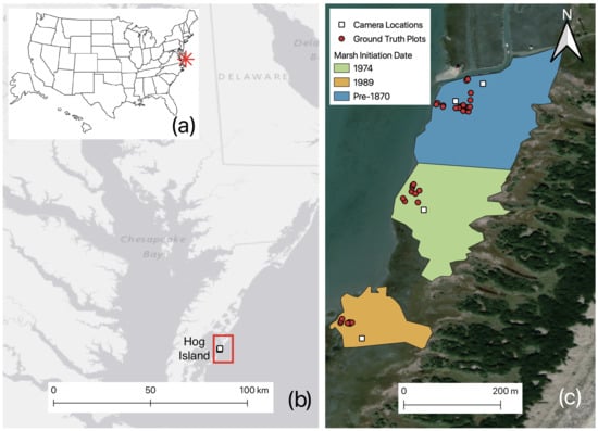
Figure 1.
(a) Location of study site in Virginia, USA, (b) location of Hog Island, (c) locations of plots and hyperspectral imaging system within the Hog Island chronosequence. Color indicates the initiation year of the marsh. For this study, groundtruth plots were established in the marshes initiated in approximately 1845, 1974 and 1989.
2.2.2. Field Imagery Collection
During the field campaigns, we collected hyperspectral imagery using the Headwall system described above mounted on a telescopic mast [51]. We placed Spectralon reference panels in the field of view and used these to convert hyperspectral imagery to reflectance. The pixel size obtained ranged from 0.2 to 3.0 cm, depending on the height of the mast and the distance of the plants from the imaging system [51]. We ensured that ground-truth plots lay within the field of view, and took biophysical measurements (as detailed below) contemporaneously at each site. Our imagery was taken from four mast locations located within the three different aged marshes (Figure 1). For validation, we used a total of 36 − 1 m ground truth plots for porewater variables and 34 − 1 m for foliar (Figure 1). We measured porewater salinity and ORP at each plot as described previously. Within 0.5 m of each plot, we clipped three culms and pooled the samples for foliar analysis after freeze-drying and homogenization on a Wiley Mill and analysis as above. We determined biomass in each plot by measuring culm density and plant height, and applying allometric equations developed separately for each age of marsh [56].
2.3. Imagery Analysis
Diagrams summarizing the workflow for the laboratory and field imagery appear in Figure 2. For the laboratory images, we used only the reflectance between 475 and 950 nm (293 total bands) in the analysis due to lower signal-to-noise (SNR) ratio at the shortest and longest wavelengths where SNR is typically lower for silicon detectors commonly used in hyperspectral imagers designed for the visible and near infra-red (VNIR). In order to isolate only pure plant pixels, for each plant, we manually selected approximately 200–300 pixels arbitrarily from each image at the center of the leaf. From these pixels, we computed the average reflectance for each plant. For field imagery, we applied a Savitzky-Golay smoothing filter [57] using and then isolated vegetation pixels by calculating the for each pixel and masking out all pixels with , in order to remove extraneous soil and water pixels. While other vegetation indices were evaluated as a mask-criterion, we found the best performance with NDVI based on visual inspection of images before and after masking. Within the plots visible in the image, we selected approximately 100 pixels for calculating the average reflectance. We applied previously published vegetation indices (Table 1) to both greenhouse and field imagery in order to examine their relationship with porewater salinity, porewater redox potential and foliar N (as a proxy for sediment nutrient status). We employed stepwise regression models, implemented in JMP Pro 14, with all potential indices and used the Akaike Information Criterion (AIC) validation [58] to select the best model. We noted, however, that these indices might not include wavelengths that would serve as the best predictors. As a result, we also explored additional wavelengths and 1st and 2nd derivatives that were potentially good predictors using an elastic net generalized regression [59].
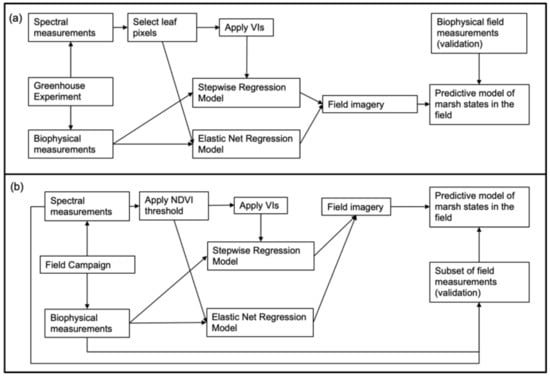
Figure 2.
Diagrams showing (a) the workflow for the analysis of the greenhouse experiment data, application to field imagery, and validation and (b) the workflow for the analysis for the field imagery.

Table 1.
Vegetation indices applied in this study.
The elastic net regression method is a shrinkage, or regularization, technique that can be used as a feature selection method when the number of predictors is much greater than the number of observations. This method constrains the number of predictor variables by adding a penalty term for the number of variables. Model coefficients that do not explain significant variance are driven toward zero and ultimately removed from the regression while regularizing the remaining coefficients [59].
Additionally, we calculated the continuum-removed reflectance between 475 and 950 nm to compare normalized absorption features between treatments. To determine the wavelengths that best predict foliar , porewater salinity, and redox potential, we developed an elastic net generalized regression for each response variable using the reflectance and first and second derivatives for the greenhouse and field imagery separately, ultimately selecting the model with the lowest AIC. We applied the equations generated from the greenhouse imagery to the field plots and then, using a linear regression analysis, compared the estimated values to measured values obtained in the field plots. We also developed an elastic net regression based on the smoothed reflectance and first and second derivatives from the field imagery. For the field imagery, our linear regression was based on dividing our samples into training (n = 28) and validation (n = 13) sets. We performed a bootstrap analysis for all models developed for both the laboratory and field imagery, in each case using 1000 bootstrap trials in order to determine confidence intervals for the coefficients, utilizing JMP Pro 14.
3. Results
3.1. Greenhouse Experiment
S. alterniflora survival rates for the high and low nutrient, low salinity, and waterlogged treatments were of pots, but were reduced to and of pots in the moderate and high salinity treatments, respectively. Porewater salinity ranged from an average of 32 ppt in the low salinity treatment to 56 ppt in the high salinity treatment (Table 2). Belowground biomass, leaf chlorophyll, foliar , foliar , and ORP were not significantly different between treatments. Aboveground biomass was highest in the low salinity treatment and lowest in the high salinity treatment. The ratio of foliar to total chlorophyll was highest in the high nutrient treatment and lowest in the low salinity treatment. Porewater salinity and foliar had a weak negative relationship with aboveground biomass (Figure 3a,c, , and , , respectively). Porewater redox had no correlation with aboveground biomass (Figure 3b, , ).
Table 2.
Mean (SE) S. alterniflora aboveground (AG) biomass (g), belowground (BG) biomass (g), foliar , aerial N (g), chlorophyll a and b (Chl, mg m), chlorophyll a and b: foliar , porewater salinity (), ORP (mV), and porewater ammonium (NH, M) per treatment from the greenhouse experiment. Unique superscripted letters indicate significant differences between treatments found in one-way ANOVA. The degrees of freedom for all are 5.
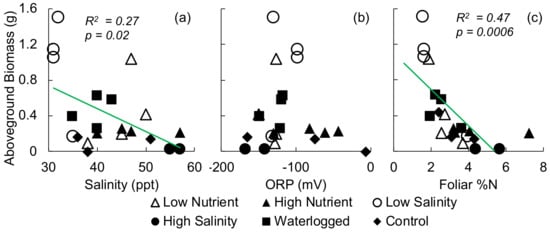
Figure 3.
Aboveground biomass versus (a) porewater salinity, (b) porewater ORP, (c) foliar . Trendline shows linear regression and statistics when the relationship was significant.
Spectra display the typical vegetation curve [73], but with pronounced differences between treatments (Figure 4a). This is particularly noticeable in the red edge slope (680–730 nm) and green peak (520–560 nm) as well as the magnitude of the near infrared (NIR) region, which is reduced in the high salinity treatment relative to the low salinity and low nutrient treatments. These differences are also visible in the continuum-removed spectra (Figure 4b), primarily in the green peak region. A summary of the values, associated errors, and predictive bands or vegetation indices for the greenhouse experiment appear in Table 3. Models developed from the greenhouse experiment ranged in values from 0.23 to 0.90 for the training data (Table 3; Figure 5a–c). Parameter estimates and confidence intervals for all models developed with the greenhouse imagery are available in Tables S1 and S2.
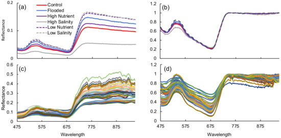
Figure 4.
(a) Average reflectance of selected leaves by treatment for the greenhouse experiment, (b) continuum removed average reflectance of selected leaves by treatment for the greenhouse experiment, (c) Spectra from field plots, (d) continuum removed spectra from field plots.
Table 3.
Results of the elastic net regressions using reflectance and 1st (‘) and 2nd (“) derivative and stepwise regression of vegetation indices for the greenhouse imagery. Validation results report greenhouse regressions applied to field imagery. * indicates significant predictor at p < 0.05, ** indicates significant predictor at p < 0.01. Factors are the significant spectral bands (nm) for the elastic net or vegetation indices for the stepwise regression.
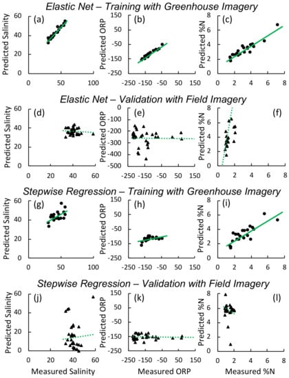
Figure 5.
Predicted versus measured values for models developed using greenhouse imagery and validated using field imagery for the elastic net models of salinity (ppt) ((a) training (d) validation), oxidation-reduction potential (ORP, mv) ((b) training, (e) validation), and foliar ((c) training, (f) validation) and for stepwise regression models of salinity (ppt) ((g) training (j) validation), oxidation-reduction potential (ORP, mv) ((h) training, (k) validation), and foliar ((i) training, (l) validation). Solid lines indicate best fit linear regression for the training set, while dashed lines indicate the regression for the validation set.
3.2. Field
Field biomass ranged from 7.8 to 569.9 g m across all sites (Table 4). Porewater salinity values from field plots ranged from 33 to 58 ppt; redox potential ranged from −222 to +162 mV; and foliar N ranged from 0.91% to 2.05% (Table 4). Field spectra exhibited a high degree of variability across sites and plots (Figure 4c) that remained even upon continuum removal (Figure 4d).
Table 4.
Average± standard deviation [minimum-maximum] for biomass (g m), height (cm), density (culms m), foliar , ORP (), and salinity () of field validation plots across three different aged marshes.
When we applied models that we developed using the greenhouse experiment imagery to the field imagery as validation, values were poor, ranging from <0.1–0.39 (Table 5) ((Figure 5d–f). In contrast, models trained on a subset of field plots had higher values for both training and validation sets: values for training sets ranged from 0.96 to 0.97 (elastic net on reflectance and 1st and 2nd derivatives; Figure 6d–f)) and to (stepwise regression on vegetation indices; Figure 6j–l)) (Table 5), while validation values ranged between 0.22 and 0.74 (elastic net) and 0.1 and 0.99 (stepwise). The foliar models had the highest value when applied to the validation set with respectively for the elastic net and for the stepwise N model. In stepwise models, WI, OSAVI, GRVI, and MSAVI2 were the best predictors of salinity, explaining of the variation in the training data and in the validation data. The models for porewater redox potential consistently had the lowest values and highest RMSE. Parameter estimates and confidence intervals for all models developed with the field appear in Tables S3 and S4. Models developed and tested using field imagery and applied back to original imagery display the characteristic heterogeneity found in such marshes (Figure 7).
Table 5.
Results of the elastic net regressions using reflectance and 1st (‘) and 2nd (“) derivative and stepwise regression on vegetation indices for the field imagery. Regressions used a subset of field imagery points, with validation data consisting of the remainder of the plots from the field imagery. * indicates significant predictor at p < 0.05, ** indicates significant predictor at p < 0.01. Factors are the significant spectral bands (nm) for the elastic net or vegetation indices for the stepwise regression.
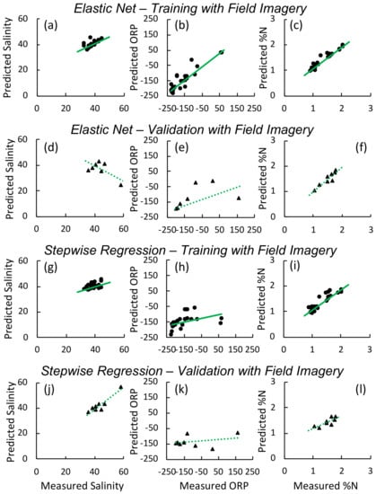
Figure 6.
Predicted versus measured values for models developed and validated using field imagery for the elastic net models of salinity (ppt) ((a) training (d) validation), oxidation-reduction potential (ORP, mv) ((b) training, (e) validation), and foliar ((c) training, (f) validation) and for stepwise regression models of salinity (ppt) ((g) training (j) validation), oxidation-reduction potential (ORP, mv) ((h) training, (k) validation), and foliar ((i) training, (l) validation). Solid lines indicate best fit linear regression for the training set, while dashed lines indicate the regression for the validation set.
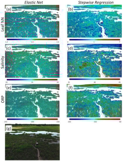
Figure 7.
Field prediction equations applied to field imagery: (a) elastic net regression for foliar , (b) stepwise VI regression for foliar , (c) elastic net regression for salinity, (d) stepwise VI regression for salinity, (e) elastic net regression for ORP, (f) stepwise regression for ORP, (g) original image. Scale bars beneath each image represent foliar (panels a and b), salinity in ppt (panels c and d), and oxidation-reduction potential (ORP) in mv (panels e and f).
4. Discussion
We successfully developed models for a range of salinity and foliar N content using both vegetation indices and reflectance, but the models based on elastic net or stepwise regression did not predict ORP well in laboratory or field validation (Figure 5). Models trained on the lab imagery were generally poor predictors when applied to field validation points, likely due to a variety of factors including differences in conditions between the field and laboratory settings, mixed pixels, as well bi-directional reflectance distribution (BRDF) effects. However, models that we developed directly from the field imagery did successfully predict foliar and salinity.
4.1. Spectral Response to Stress
Spectral detection of vegetation relies on several key absorption features that contribute to a distinctive ‘vegetation curve’ (as seen in Figure 4). Within the visible spectrum, reflectance is primarily dominated by leaf pigments in the palisade mesophyll such as chlorophyll a and b, carotenes, or anthocyanins [74]. This region may also be useful as a measure of stress (or senescence) as chlorophyll decreases and other pigments become visible [75]. The high reflectance typically observed in the near infrared region (NIR, approximately 700–1200 nm) may be an adaptation to prevent overheating [73] with the steep increase between the red and the NIR (the ’red edge’) acting as another metric of potential stress. While using vegetation indices seeks to minimize confounding factors and heighten useful variation within the spectra, they are also limited to a narrow range of bands which might not include wavelengths that could be better predictors of stress conditions. Consequently, in this study, we used two approaches— the stepwise regression method to test existing indices, as well as the elastic net regression, which extracted other predictor wavelengths. For the models developed from the field imagery, stepwise regression proved a more significant predictor for foliar N and salinity. Many vegetation indices have been developed to predict either foliar or leaf greenness, which tend to be closely connected, and the predictive indices included in this model reflect this. Salinity and redox potential have fewer established indices, primarily developed for upland, salt-sensitive plants, so may not be as effective in this context.
4.2. Nitrogen
While detection of foliar N has been widely analyzed in agricultural and terrestrial systems, there are relatively few studies in wetlands [76,77]. Field leaf ( to ) was generally much lower than the content in the greenhouse-grown plants ( to ), providing little overlap in values across datasets. It is likely that the potting mix enhanced N sufficiently that there was little variation among treatments, with only marginally higher foliar in the high salinity and high nutrient treatments (, Table 2). In high salinity conditions, the minimum required tissue concentration of N increases, likely due to the production and accumulation of the nitrogen-based osmoregulatory compounds proline and glycinebetaine, which promote salt tolerance [44,78]. We observed the highest foliar in the high salinity treatment, and a significant negative relationship between aboveground biomass and foliar , possibly driven by the interacting impact of salinity and nitrogen (Figure 3). Differences in leaf physiology, such as the accumulation of osmoregulatory compounds or pigments, may influence reflectance and be detectable as changes in reflectance spectra. Foliar N is often correlated with chlorophyll content, and numerous studies have linked chlorophyll absorption features and the red edge region with foliar N content [37,76,79]. The high observed ratio in the high N treatment suggests that additional N was shunted towards compounds other than photosynthetic pigments; while the lower value in the low salinity treatment was driven by moderate chlorophyll concentration and lower , perhaps diluted by the additional tissue growth. Salicornia virginica fertilized with N demonstrated lower reflectance at 555 nm and 680 nm and steeper red-edge slopes, a shift detectable using vegetation indices including PRI [76] and normalized difference indices using the first order derivatives at 1235 nm and 549 nm have been shown to correlate with foliar N in Schoenoplectus acutus [77].
Likewise, NDVI may correlate with foliar N in wheat [80]. We had similar success in predicting foliar N in both lab and field studies, with significant predictor wavelengths falling near chlorophyll absorption or fluorescence features (the first derivatives at 651 nm and 672 nm; greenhouse experiment, elastic net); however, no wavelengths associated with the red edge were identified. These findings may align with the variation in chlorophyll relative to other N-containing compounds in the mesophyll. In contrast, for field-derived models, the second derivative at 415 nm was also a predictor of N content, as previously shown by Read et al. [79], where decreased reflectance at 410 nm was associated with N stress in cotton plants. The inability to apply greenhouse-derived models to the field may stem from the lack of overlap in foliar N values for the training data and suggests perhaps a non-linearity in the response over a larger range of N content. However, additional predictor wavelengths from the field imagery were located in the NIR region (907, 908, and 803 nm based on elastic net; Table 5) and to some extent were coincidental with those used to develop indices that were selected as significant using the stepwise regression. These indices, including those commonly used to detect green biomass (NDVI, MSAVI2, GRVI and OSAVI [63,70,72]), were significant predictors of foliar N. In the field leaf model, the vegetation indices included WI (using wavelengths 900 and 970 nm), OSAVI (using wavelengths 800 and 670 nm), and MSAVI2 (using wavelengths 800 and 680 nm). These suggest a common biophysical mechanism induced by variable N status that alters reflectance in this region.
4.3. Salinity
The range of porewater salinity found in the field (33–58 ppt) was replicated in the lab (31–57 ppt), suggesting that any salinity-induced impacts to plants may be comparable. Likewise, the negative relationship between salinity and biomass in the greenhouse experiment is consistent with prior work [20,46,78]. High salinity can result in reduced stomatal conductance and CO assimilation [81], increased leaf respiration [82], and accumulation of osmoregulatory compounds in tissues [44]. Longstreth and Strain [83] found that increasing salinity resulted in higher leaf xylem pressure and higher specific leaf weight, potentially due to increases in mesophyll thickness developed as a mechanism for salt avoidance. Thicker mesophyll results in a greater internal leaf area where gaseous exchange takes place, lowering resistance to CO uptake and possibly compensating for salinity-induced resistance to CO uptake [84]. As scattering in the mesophyll contributes to NIR reflectance [73], changes in leaf structure could be responsible for reduced NIR reflectance at higher salinity (Figure 4).
In salt-sensitive plants, reflectance in the NIR region is lower with salinity stress, likely due to cell structure damage [85]. However, in halophytes, while NIR reflectance may also decrease at higher salinity due to cell structure damage, at moderate salinity, reflectance in this region may increase [85]. Our results suggest that S. alterniflora may behave like a more salt-sensitive species, as we observed a substantial decrease in NIR reflectance as the salinity increased from low to high (Figure 4), although we note that the salinity in our study encompassed a greater range than in Zhang et al. who found a relatively weak relationship between salinity and vegetation indices [85]. We also note that for our field values, one relatively high salinity value (58 ppt) appears to have an inordinate impact on the derived relationships. However, removal of this point still yields significant relationships, albeit with a reduced (stepwise regression p = 0.0009, = 0.27; elastic net p = 0.0004, = 0.3). Additionally, secreted salt crystalloids (e.g., [78]) were visible on leaves at higher salinity treatments and may have influenced the spectra. In Avicennia germinans, Esteban et al. [86] found that the reflectance in the blue (400–500 nm) and red (630–680 nm) regions increased when leaves were covered in salt crystalloids; however, we observed the reverse in this study. Zhang et al. [85] found that the regions of 395–410 nm, 483–507 nm, 632–697 nm, 731–762 nm, 812–868 nm, 884–909 nm, and 918–930 nm were the wavelengths most sensitive to salt stress and suggests that photosynthetic pigments are highly affected by salt stress. In this study, two of three, and five of eleven predictor wavelengths for salinity from the greenhouse and field experiments respectively were in the visible range, but mostly outside of the ranges indicated above. This could be due to differences in species and biological responses to salinity stress; Zhang et al. [85] found that the spectral response to salinity was species dependent, and did not investigate S. alterniflora specifically. In the greenhouse study, OSAVI2 appears as a significant predictor in both the and salinity models, potentially illustrating the connection between salt stress and nitrogen storage. In our field study, a combination of WI, NDVI, WDR-NDVI were the best predictors of porewater salinity, each explaining about of the variation in the field training and validation sets. The stepwise field model for salinity used the vegetation indices NDVI (800 and 860 nm), WI (900 and 970 nm), and WDR NDVI (800 and 680 nm) while the elastic net model selected similar wavelengths 803, 699, and 916 nm. These similarities highlight the importance of absorption features centered around these wavelengths. The WI is sensitive to leaf water content [62], which responds to salt stress in S. alterniflora [83]. NDVI and WDR-NDVI are sensitive to leaf greenness and chlorophyll concentrations [72], which may decrease with salinity stress as plants shunt available N to organic compounds needed for osmoregulation.
4.4. Waterlogging
S. alterniflora can tolerate substantially lower redox potentials than those achieved in our greenhouse experiment (−167 mV to −43 mV), beginning to show symptoms of oxygen deficiency only below −200 mV [87] and explaining the lack of an observed relationship between biomass and redox (Figure 3b). However, the wider range of porewater redox potential in the field (−222 mV−+161.5 mV) was likely sufficient to generate the hypoxic condition that limits essential plant functions. Many wetland plants, adapted to the anaerobic conditions that occur in flooded soils, contain aerenchyma to transport oxygen from aerial parts to flooded roots where it supports aerobic root metabolism and oxidation of the rhizosphere [88]. In S. alterniflora, aerenchyma development may be induced by low oxygen conditions [44,89,90]. However, in extremely waterlogged soils, aerenchyma transport is not always sufficient for entirely aerobic metabolism in the roots [87,88] and the metabolic pathway switches to fermentation where the enzyme alcohol dehydrogenase (ADH) is used to reduce pyruvate to ethanol [87,91]. Low redox conditions also reduce root elongation and a smaller root system that may be unable to support the shoot [88]. While many symptoms of hypoxia take place belowground, ATP yield is increased at the expense of glucose consumption, resulting in higher respiration and decreased overall growth [87] and reduced NH uptake may decrease photosynthesis and foliar N [88,92].
Combined, these physical and biochemical effects induce overall stress symptoms including stomatal closure and limited gas exchange and photosynthesis [88] with a visible spectral response previously observed only in terrestrial plants such as Acer rubrum and field crops [42,43]. These studies found good correlation between redox and select wavelengths in the visible region, and a reduced red edge shift towards longer wavelengths over time in waterlogged plants, possibly due to inhibition of maturation and lower chlorophyll content in waterlogged plants [42,43]. In our greenhouse experiment, the second derivatives at 573 and 755 nm, which are within or near these previously identified regions [42,43], predicted porewater redox along with the derivative at 830 nm and the second derivative at 918 and 909 nm. Both the WI, which uses wavelengths 900 and 970 nm, and the second derivative at 909 nm from the elastic net model were selected and include features in the water absorption region, suggesting similarities in response. However, this model did not translate well to the field imagery (Table 3) probably due to the lack of overlap in values between lab and field ORP.
Models developed to detect ORP using our field imagery did not include wavelengths that had been previously identified in the literature for other species. The second derivatives at 463, 473, 795, 809, 830, and 961 nm as well as the first derivative at 884 nm were predictive of porewater redox in the field (), but only explained of the variation upon validation. PRI was developed as an indication of photosynthetic efficiency, which is often correlated with plant stress [68] and while this index emerged as the best VI to predict ORP, it was not successfully validated (Table 3). Often, under stress conditions, photosynthetic capacity decreases and the amount of incoming radiation is greater than is required for photosynthesis; in this case, under stress, excess energy is dissipated through the xanthophyll cycle. PRI incorporates 531 nm, which is linked to the xanthophyll cycle, and is inversely related to photosynthetic light use efficiency [67]. While PRI has not been used previously to detect waterlogging stress, it has been used to detect salt stress in a coastal shrub [93], and in the field, plants are subject to numerous stressors acting in tandem. Future studies could focus on generating a wider range of redox potential in a controlled setting to further elucidate spectral characteristics of this particular stress response.
4.5. Limitations of Models
Our inability to translate models developed in the lab to field imagery is likely due to a combination of factors including differences in illumination and view angle, effects of canopy structure and concomitant stressors, differences in scale, and potentially mixed pixels in the field imagery. With regard to differences in scale, in the laboratory, pixel sizes were approximately 1.2 mm. In field settings, pixel sizes varied over the image due to the oblique geometry of our imaging system. That geometry also varied with the height of our imaging system on the mast above the marsh surface. Typical field plots were usually within 50 meters or less. As a result, typical marsh hyperspectral imagery pixels in our study site were acquired at a spatial resolution ranging from 0.2 to 3 cm. A more complete summary of the capabilities of our imaging system appears in [51]. This difference in pixel size between the laboratory and the field may contribute to the lack of agreement between models, as the laboratory measurements may pick up finer details of the leaf surface.
Other barriers to successfully translating models stemmed from issues associated with calibration from the the white Spectralon reference panels, which are not perfectly Lambertian, and since the illumination angle and viewing angle are different in the lab and the field, it likely influences the conversion to reflectance. However, a correction for this can be carried out for future studies. Additionally, view angle and canopy structure have strong influences on reflectance due to multiple light scattering, leaf layering, and shading [73]. Future models could make use of radiative transfer models in order to account for this geometry. We minimized mixed pixels in the laboratory setting by hand-selecting areas of leaf, but in spite of the application of the NDVI filter to the field imagery to isolate vegetation, mixed pixels containing some sediment are likely given the larger pixel size in the field. This suggests that future refinements of these models must incorporate varying scales of imagery to assess the potential impact of mixed pixels.
Further, in a field setting, multiple stressors are acting simultaneously, leading to a composite impact that is harder to isolate using a model developed for a single response variable. For example, as demonstrated for our laboratory experiment and by others (e.g., [94,95]), high salinity may cause plants to accumulate nitrogen but at the same time stunt growth, leading to increased foliar N. Likewise, waterlogging and high salinity will decrease plant growth, leading to lower biomass and plant allometric relationships, in turn impacting the spectral response. Future work to incorporate plant biomass, allometry and external stressors will be useful to further untangle these relationships and their synergistic influence on reflectance.
5. Conclusions
This study was the first step in developing indicators of salt marsh health using remote sensing. Overall, models were successful for predicting a range of salinity and leaf N content in both the laboratory and the greenhouse individually. Generally, models developed from previously published vegetation indices were more successful at predicting salinity and foliar than models developed from an elastic net regression approach. The failure to develop adequate models for ORP suggests the need for additional study to better isolate this stressor and understand how the plant physiologic and structural responses translate to the spectral reflectance. Although models developed from a controlled greenhouse experiment did not translate well to field imagery, likely due to a combination of factors including differences in environmental conditions, mixed pixels in the field imagery, and BRDF effects, future experiments could better correct for these factors. Further development of these spectral models may provide an efficient way to evaluate marsh states and stressors in the field at a large scale, which can inform marsh management decisions.
Supplementary Materials
The following are available online at https://www.mdpi.com/2072-4292/12/18/2938/s1.
Author Contributions
Conceptualization, S.B.G., A.C.T., C.M.B. and D.T.O.; methodology, S.B.G., A.C.T., C.M.B. and D.T.O.; software, S.B.G., R.S.E., C.S.L., G.P.B.; validation, S.B.G., R.S.E., C.S.L., G.P.B., A.C.T., C.M.B. and D.T.O.; formal analysis, S.B.G., A.C.T., C.M.B.; investigation, S.B.G., R.S.E., C.S.L., G.P.B., A.C.T., C.M.B. and D.T.O.; resources, A.C.T. and C.M.B.; data curation, S.B.G., R.S.E., C.S.L., G.P.B., A.C.T., C.M.B.; writing, S.B.G., A.C.T., C.M.B., D.T.O.; visualization, S.B.G., R.S.E., C.S.L., G.P.B.; supervision, A.C.T., C.M.B., and D.T.O.; project administration, A.C.T. and C.M.B.; funding acquisition, A.C.T. and C.M.B. All authors have read and agreed to the published version of the manuscript.
Funding
A.C.T. and C.M.B. gratefully acknowledge support of their work by the National Geographic Explorers program under Grant NGS-382R-18. The authors are also grateful for support provided by NSF DEB Grants #1237733 and #1832221 (VCR-LTER), which contributed to the fieldwork described in this paper. Additional funding was provided by the College of Science at the Rochester Institute of Technology.
Acknowledgments
The authors are grateful for the assistance of Ryan Brett, Sydney VanWinkle, Sarah Ponte Cabral, Patrick Minnig, Nelmy Robles-Serrano, Marke Foote, David Lee, Cora Johnston, Donna Fauber, Karen McGlathery, John Porter, and Avery Miller.
Conflicts of Interest
The authors declare no conflict of interest. The funders had no role in the design of the study; in the collection, analyses, or interpretation of data; in the writing of the manuscript, or in the decision to publish the results.
Abbreviations
The following abbreviations are used in this manuscript:
| MDPI | Multidisciplinary Digital Publishing Institute |
| NDVI | Normalized Difference Vegetation Index |
| NIR | Near Infrared |
| BRDF | Bidirectional Reflectance Distribution Function |
References
- Morris, J.T.; Sundareshwar, P.V.; Nietch, C.T.; Kjerfve, B.; Cahoon, D.R. Responses of Coastal Wetlands to Rising Sea Level. Ecology 2002, 83, 2869–2877. [Google Scholar] [CrossRef]
- McKee, K.L.; Mendelssohn, I.A.; Materne, M.D. Acute salt marsh dieback in the Mississippi River deltaic plain: A drought-induced phenomenon? Glob. Ecol. Biogeogr. 2004, 13, 65–73. [Google Scholar] [CrossRef]
- Gedan, K.B.; Silliman, B.R.; Bertness, M.D. Centuries of Human-Driven Change in Salt Marsh Ecosystems. Annu. Rev. Mar. Sci. 2009, 1, 117–141. [Google Scholar] [CrossRef] [PubMed]
- Hughes, A.L.H.; Wilson, A.M.; Morris, J.T. Hydrologic variability in a salt marsh: Assessing the links between drought and acute marsh dieback. Estuarine Coast. Shelf Sci. 2012, 111, 95–106. [Google Scholar] [CrossRef]
- Alber, M.; Swenson, E.M.; Adamowicz, S.C.; Mendelssohn, I.A. Salt Marsh Dieback: An overview of recent events in the US. Estuarine Coast. Shelf Sci. 2008, 80, 1–11. [Google Scholar] [CrossRef]
- Bertness, M.D.; Silliman, B.R. Consumer Control of Salt Marshes Driven by Human Disturbance. Conserv. Biol. 2008, 22, 618–623. [Google Scholar] [CrossRef]
- Boesch, D.; Turner, R. Dependence of Fishery Species on Salt Marshes: The Role of Food and Refuge. Estuaries 1984, 7, 460–468. [Google Scholar] [CrossRef]
- Barbier, E.B.; Koch, E.W.; Silliman, B.R.; Hacker, S.D.; Wolanski, E.; Primavera, J.; Granek, E.F.; Polasky, S.; Aswani, S.; Cramer, L.A.; et al. Coastal ecosystem-based management with nonlinear ecological functions and values. Science 2008, 319, 321–323. [Google Scholar] [CrossRef]
- Koch, M.S.; Mendelssohn, I.A.; McKee, K.L. Mechanism for the hydrogen sulfide-induced growth limitation in wetland macrophytes. Limnol. Oceanogr. 1990, 35, 399–408. [Google Scholar] [CrossRef]
- Morgan, P.A.; Burdick, D.M.; Short, F.T. The Functions and Values of Fringing Salt Marshes in Northern New England, USA. Estuaries Coasts 2009, 32, 483–495. [Google Scholar] [CrossRef]
- Chmura, G.L.; Anisfeld, S.C.; Cahoon, D.R.; Lynch, J.C. Global carbon sequestration in tidal, saline wetland soils. Glob. Biogeochem. Cycles 2003, 17, 1111. [Google Scholar] [CrossRef]
- Chmura, G.L. What do we need to assess the sustainability of the tidal salt marsh carbon sink? Ocean. Coast. Manag. 2013, 83, 25–31. [Google Scholar] [CrossRef]
- Mcleod, E.; Chmura, G.L.; Bouillon, S.; Salm, R.; Björk, M.; Duarte, C.M.; Lovelock, C.E.; Schlesinger, W.H.; Silliman, B.R. A blueprint for blue carbon: Toward an improved understanding of the role of vegetated coastal habitats in sequestering CO2. Front. Ecol. Environ. 2011, 9, 552–560. [Google Scholar] [CrossRef]
- Hopkinson, C.; Cai, W.J.; Hu, X. Carbon Sequestration in Wetland Dominated Coastal Systems—A Global Sink of Rapidly Diminishing Magnitude. Curr. Opin. Environ. Sustain. 2012, 4, 186–194. [Google Scholar] [CrossRef]
- Turner, R.E.; Howes, B.L.; Teal, J.M.; Milan, C.S.; Swenson, E.M.; Tonerb, D.D.G. Salt marshes and eutrophication: An unsustainable outcome. Limnol. Oceanogr. 2009, 54, 1634–1642. [Google Scholar] [CrossRef]
- Turner, R.E.; Swenson, E.M.; Milan, C.S.; Lee, J.M.; Oswald, T.A. Below-ground biomass in healthy and impaired salt marshes. Ecol. Res. 2004, 19, 29–35. [Google Scholar] [CrossRef]
- Deegan, L.A.; Johnson, D.S.; Warren, R.S.; Peterson, B.J.; Fleeger, J.W.; Fagherazzi, S.; Wollheim, W.M. Coastal eutrophication as a driver of salt marsh loss. Nature 2012, 490, 388–392. [Google Scholar] [CrossRef]
- Hester, M.W.; Mendelssohn, I.A.; McKee, K.L. Intraspecific Variation in Salt Tolerance and Morphology in Panicum hemitomon and Spartina alterniflora (Poaceae). Int. J. Plant Sci. 1998, 159, 127–138. [Google Scholar] [CrossRef]
- Linthurst, R.A.; Seneca, E.D. Aeration, Nitrogen and Salinity as Determinants of Spartina alterniflora Loisel. Growth Response. Estuaries 1981, 4, 53. [Google Scholar] [CrossRef]
- Brown, C.; Pezeshki, S.; DeLaune, R. The effects of salinity and soil drying on nutrient uptake and growth of Spartina alterniflora in a simulated tidal system. Environ. Exp. Bot. 2006, 58, 140–148. [Google Scholar] [CrossRef]
- Artigas, F.J.; Yang, J. Spectral discrimination of marsh vegetation types in the New Jersey Meadowlands, USA. Wetlands 2006, 26, 271–277. [Google Scholar] [CrossRef]
- Bachmann, C.; Donato, T.; Lamela, G.; Rhea, W.; Bettenhausen, M.; Fusina, R.; Du Bois, K.; Porter, J.; Truitt, B. Automatic classification of land cover on Smith Island, VA, using HyMAP imagery. IEEE Trans. Geosci. Remote. Sens. 2002, 40, 2313–2330. [Google Scholar] [CrossRef]
- Bachmann, C.; Bettenhausen, M.; Fusina, R.; Donato, T.; Russ, A.; Burke, J.; Lamela, G.; Rhea, W.; Truitt, B.; Porter, J. A credit assignment approach to fusing classifiers of multiseason hyperspectral imagery. IEEE Trans. Geosci. Remote. Sens. 2003, 41, 2488–2499. [Google Scholar] [CrossRef]
- Cheng, W.C.; Chang, J.C.; Chang, C.P.; Su, Y.; Tu, T.M. A Fixed-Threshold Approach to Generate High-Resolution Vegetation Maps for IKONOS Imagery. Sensors 2008, 8, 4308–4317. [Google Scholar] [CrossRef] [PubMed]
- Klemas, V.V. Remote Sensing of Wetlands: Case Studies Comparing Practical Techniques. J. Coast. Res. 2011, 27. [Google Scholar] [CrossRef]
- Hladik, C.; Schalles, J.; Alber, M. Salt marsh elevation and habitat mapping using hyperspectral and LIDAR data. Remote. Sens. Environ. 2013, 139, 318–330. [Google Scholar] [CrossRef]
- Byrd, K.B.; O’Connell, J.L.; Di Tommaso, S.; Kelly, M. Evaluation of sensor types and environmental controls on mapping biomass of coastal marsh emergent vegetation. Remote. Sens. Environ. 2014, 149, 166–180. [Google Scholar] [CrossRef]
- Byrd, K.B.; Ballanti, L.; Thomas, N.; Nguyen, D.; Holmquist, J.R.; Simard, M.; Windham-Myers, L. A remote sensing-based model of tidal marsh aboveground carbon stocks for the conterminous United States. Isprs J. Photogramm. Remote. Sens. 2018, 139, 255–271. [Google Scholar] [CrossRef]
- DiGiacomo, A.E.; Bird, C.N.; Pan, V.G.; Dobroski, K.; Atkins-Davis, C.; Johnston, D.W.; Ridge, J.T. Modeling Salt Marsh Vegetation Height Using Unoccupied Aircraft Systems and Structure from Motion. Remote Sens. 2020, 12, 2333. [Google Scholar] [CrossRef]
- Ramsey, E., III; Rangoonwala, A. Leaf Optical Property Changes Associated with the Occurrence of Spartina alterniflora Dieback in Coastal Louisiana Related to Remote Sensing Mapping. Photogramm. Eng. Remote. Sens. 2005, 71, 299–311. [Google Scholar] [CrossRef]
- Ramsey, E., III; Rangoonwala, A. Canopy reflectance related to marsh dieback onset and progression in coastal Louisiana. Photogramm. Eng. Remote. Sens. 2006, 22, 641–652. [Google Scholar] [CrossRef]
- Ramsey, E.; Rangoonwala, A. Characterizing the marsh dieback spectral response at the plant and canopy level with hyperspectral and temporal remote sensing data. In Proceedings of the 2008 IEEE/OES US/EU-Baltic International Symposium, Tallinn, Estonia, 27–29 May 2008; IEEE: Piscataway, NJ, USA, 2008; pp. 1–8. [Google Scholar]
- Marsh, A.; Blum, L.K.; Christian, R.R.; Ramsey, E.; Rangoonwala, A. Response and resilience of Spartina alterniflora to sudden dieback. J. Coast. Conserv. 2016, 20, 335–350. [Google Scholar] [CrossRef]
- Miller, G.; Morris, J.; Wang, C. Mapping salt marsh dieback and condition in South Carolina’s North Inlet-Winyah Bay National Estuarine Research Reserve using remote sensing. Aims Environ. Sci. 2017, 4, 677–689. [Google Scholar] [CrossRef]
- Badura, G.P.; Bachmann, C.M.; Tyler, A.C.; Goldsmith, S.; Eon, R.S.; Lapszynski, C.S. A Novel Approach for Deriving LAI of Salt Marsh Vegetation Using Structure From Motion and Multiangular Spectra. IEEE J. Sel. Top. Appl. Earth Obs. Remote. Sens. 2019, 12, 599–613. [Google Scholar] [CrossRef]
- Eon, R.S.; Goldsmith, S.; Bachmann, C.M.; Tyler, A.C.; Lapszynski, C.S.; Badura, G.P.; Osgood, D.T.; Brett, R. Retreival of salt marsh above-ground biomass from high-spatial resolution, multi-view hyperspectral imagery using PROSAIL. Remote Sens. 2019, 11, 1385. [Google Scholar] [CrossRef]
- LaCapra, V.C.; Melack, J.M.; Gastil, M.; Valeriano, D. Remote sensing of foliar chemistry of inundated rice with imaging spectrometry. Remote Sens. Environ. 1996, 55, 50–58. [Google Scholar] [CrossRef]
- Tian, Y.; Yao, X.; Yang, J.; Cao, W.; Zhu, Y. Extracting Red Edge Position Parameters from Ground- and Space-Based Hyperspectral Data for Estimation of Canopy Leaf Nitrogen Concentration in Rice. Plant Prod. Sci. 2011, 14, 270–281. [Google Scholar] [CrossRef]
- He, L.; Song, X.; Feng, W.; Guo, B.B.; Zhang, Y.S.; Wang, Y.H.; Wang, C.Y.; Guo, T.C. Improved remote sensing of leaf nitrogen concentration in winter wheat using multi-angular hyperspectral data. Remote Sens. Environ. 2016, 174, 122–133. [Google Scholar] [CrossRef]
- O’Connell, J.L.; Mishra, D.R.; Cotten, D.L.; Wang, L.; Alber, M. The Tidal Marsh Inundation Index (TMII): An inundation filter to flag flooded pixels and improve MODIS tidal marsh vegetation time-series analysis. Remote Sens. Environ. 2017, 201, 34–46. [Google Scholar] [CrossRef]
- Zhang, M.; Ustin, S.L.; Rejmankova, E.; Sanderson, E.W. Monitoring Pacific Coast Salt Marshes Using Remote Sensing. Ecol. Appl. 1997, 7, 1039–1053. [Google Scholar] [CrossRef]
- Anderson, J.E.; Perry, J.E. Characterization of wetland plant stress using leaf spectral reflectance: Implications for wetland remote sensing. Wetlands 1996, 16, 477–487. [Google Scholar] [CrossRef]
- Smith, K.L.; Steven, M.D.; Colls, J.J. Spectral responses of pot-grown plants to displacement of soil oxygen. Int. J. Remote. Sens. 2004, 25, 4395–4410. [Google Scholar] [CrossRef]
- Naidoo, G.; Mckee, K.L.; Mendelssohn, I.A. Anatomical and metabolic responses to waterlogging and salinity in Spartina alterniflora and S. patens (Poaceae). Am. J. Bot. 1992, 79, 765–770. [Google Scholar] [CrossRef]
- MacTavish, R.M.; Cohen, R.A. A Simple, Inexpensive, and Field-Relevant Microcosm Tidal Simulator for Use in Marsh Macrophyte Studies. Appl. Plant Sci. 2014, 2, 1400058. [Google Scholar] [CrossRef] [PubMed]
- MacTavish, R.M.; Cohen, R.A. Water column ammonium concentration and salinity influence nitrogen uptake and growth of Spartina alterniflora. J. Exp. Mar. Biol. Ecol. 2017, 488, 52–59. [Google Scholar] [CrossRef]
- Berg, P.; McGlathery, K.J. A high-resolution pore water sampler for sandy sediments. Limnol. Oceanogr. 2001, 46, 203–210. [Google Scholar] [CrossRef]
- Solórzano, L. Determination of ammonia in natural waters by the phenolhypochlorite method. Limnol. Oceanogr. 1969, 14, 799–801. [Google Scholar] [CrossRef]
- Lichtenhaler, H.; Wellburn, A.R. Determinations of total carotenoids and chlorophylls a and b of leaf extracts in different solvents. Biochem. Soc. Trans. 1983, 11, 591–592. [Google Scholar] [CrossRef]
- Tukey, J.W. Comparing individual means in the analysis of variance. Biometrics 1949, 99–114. [Google Scholar] [CrossRef]
- Bachmann, C.M.; Eon, R.S.; Lapszynski, C.S.; Badura, G.P.; Vodacek, A.; Hoffman, M.J.; McKeown, D.; Kremens, R.L.; Richardson, M.; Bauch, T.; et al. A Low-Rate Video Approach to Hyperspectral Imaging of Dynamic Scenes. J. Imaging 2019, 5, 6. [Google Scholar] [CrossRef]
- Day, F.P.; Crawford, E.R.; Dilustro, J.J. Aboveground Plant Biomass Change along a Coastal Barrier Island Dune Chronosequence over a Six-Year Period. J. Torrey Bot. Soc. 2001, 128, 197. [Google Scholar] [CrossRef]
- Hayden, B.; Dueser, J.; Shugart, H. Long Term Research at the Virginia Coast Reserve: Modeling a highly dynamic environment. Bioscience 1991, 41, 310–318. [Google Scholar] [CrossRef]
- Walsh, J.P. Low Marsh Succession along an Over-Wash Salt Marsh Chronosequence. Ph.D. Thesis, University of Virginia, Charlottesville, VA, USA, 1998. [Google Scholar]
- Tyler, A.C.; Zieman, J.C. Patterns of development in the creekbank region of a barrier island Spartina alterniflora marsh. Mar. Ecol. Prog. Ser. 1999, 180, 161–177. [Google Scholar] [CrossRef]
- Goldsmith, S. Decadal Changes in Salt Marsh Succession and Assessing Salt Marsh Vulnerability Using High-Resolution Hyperspectral Imagery; Rochester Institute of Technology, ProQuest Dissertations: Rochester, NY, USA, 2019. [Google Scholar]
- Savitzky, A.; Golay, M.J. Smoothing and differentiation of data by simplified least squares procedures. Anal. Chem. 1964, 36, 1627–1639. [Google Scholar] [CrossRef]
- Akaike, H. Information Theory and an Extension of the Maximum Likelihood Principle. In Selected Papers of Hirotugu Akaike; Parzen, E., Tanabe, K., Kitagawa, G., Eds.; Springer Series in Statistics; Springer: New York, NY, USA, 1998; pp. 199–213. [Google Scholar] [CrossRef]
- Zou, H.; Hastie, T. Regularization and variable selection via the elastic net. J. R. Stat. Soc. Ser. B (Stat. Methodol.) 2005, 67, 301–320. [Google Scholar] [CrossRef]
- Main, R.; Cho, M.A.; Mathieu, R.; O’Kennedy, M.M.; Ramoelo, A.; Koch, S. An investigation into robust spectral indices for leaf chlorophyll estimation. ISPRS J. Photogramm. Remote. Sens. 2011, 66, 751–761. [Google Scholar] [CrossRef]
- Tucker, C.J. Red and photographic infrared linear combinations for monitoring vegetation. Remote. Sens. Environ. 1979, 8, 127–150. [Google Scholar] [CrossRef]
- Penuelas, J.; Pinol, J.; Ogaya, R.; Filella, I. Estimation of plant water concentration by the reflectance Water Index WI (R900/R970). Int. J. Remote. Sens. 1997, 18, 2869–2875. [Google Scholar] [CrossRef]
- Haboudane, D.; Miller, J.R.; Tremblay, N.; Zarco-Tejada, P.J.; Dextraze, L. Integrated narrow-band vegetation indices for prediction of crop chlorophyll content for application to precision agriculture. Remote Sens. Environ. 2002, 81, 416–426. [Google Scholar] [CrossRef]
- Wu, C.; Niu, Z.; Tang, Q.; Huang, W. Estimating chlorophyll content from hyperspectral vegetation indices: Modeling and validation. Agric. For. Meteorol. 2008, 148, 1230–1241. [Google Scholar] [CrossRef]
- Daughtry, C. Estimating Corn Leaf Chlorophyll Concentration from Leaf and Canopy Reflectance. Remote Sens. Environ. 2000, 74, 229–239. [Google Scholar] [CrossRef]
- Ju, C.H.; Tian, Y.C.; Yao, X.; Cao, W.X.; Zhu, Y.; Hannaway. Estimating Leaf Chlorophyll Content Using Red Edge Parameters. Pedosphere 2010, 20, 633–644. [Google Scholar] [CrossRef]
- Gamon, J.A.; Peñuelas, J.; Field, C.B. A narrow-waveband spectral index that tracks diurnal changes in photosynthetic efficiency. Remote Sens. Environ. 1992, 41, 35–44. [Google Scholar] [CrossRef]
- Thenot, F.; Méthy, M.; Winkel, T. The Photochemical Reflectance Index (PRI) as a water-stress index. Int. J. Remote. Sens. 2002, 23, 5135–5139. [Google Scholar] [CrossRef]
- Jordan, C.F. Derivation of Leaf-Area Index from Quality of Light on the Forest Floor. Ecology 1969, 50, 663–666. [Google Scholar] [CrossRef]
- Motohka, T.; Nasahara, K.N.; Oguma, H.; Tsuchida, S. Applicability of Green-Red Vegetation Index for Remote Sensing of Vegetation Phenology. Remote Sens. 2010, 2, 2369–2387. [Google Scholar] [CrossRef]
- Haboudane, D. Hyperspectral vegetation indices and novel algorithms for predicting green LAI of crop canopies: Modeling and validation in the context of precision agriculture. Remote Sens. Environ. 2004, 90, 337–352. [Google Scholar] [CrossRef]
- Gitelson, A.A. Wide Dynamic Range Vegetation Index for Remote Quantification of Biophysical Characteristics of Vegetation. J. Plant Physiol. 2004, 161, 165–173. [Google Scholar] [CrossRef]
- Jensen, J.R. Remote Sensing of the Environment: An Earth Resource Perspective, 2nd ed.; Pearson: Upper Saddle River, NJ, USA, 2006. [Google Scholar]
- Hilker, T.; Coops, N.C.; Nesic, Z.; Wulder, M.A.; Black, A.T. Instrumentation and approach for unattended year round tower based measurements of spectral reflectance. Comput. Electron. Agric. 2007, 56, 72–84. [Google Scholar] [CrossRef]
- Knipling, E. Physical and physiological basis for the reflectance of visible and near-infrared radiation from vegetation. Remote Sens. Environ. 1970, 3, 155–159. [Google Scholar] [CrossRef]
- Siciliano, D.; Wasson, K.; Potts, D.C.; Olsen, R. Evaluating hyperspectral imaging of wetland vegetation as a tool for detecting estuarine nutrient enrichment. Remote Sens. Environ. 2008, 112, 4020–4033. [Google Scholar] [CrossRef]
- O’Connell, J.L.; Byrd, K.B.; Kelly, M. Remotely-Sensed Indicators of N-Related Biomass Allocation in Schoenoplectus acutus. PLoS ONE 2014, 9, e90870. [Google Scholar] [CrossRef] [PubMed]
- Bradley, P.; Morris, J. The influence of salinity on the kinetics of NH4+ uptake in Spartina alterniflora. Oecologia 1991, 85, 375–380. [Google Scholar] [CrossRef] [PubMed]
- Read, J.J.; Tarpley, L.; McKinion, J.M.; Reddy, K.R. Narrow-Waveband Reflectance Ratios for Remote Estimation of Nitrogen Status in Cotton. J. Environ. Qual. 2002, 31, 1442. [Google Scholar] [CrossRef]
- Cabrera-Bosquet, L.; Molero, G.; Stellacci, A.; Bort, J.; Nogués, S.; Araus, J. NDVI as a potential tool for predicting biomass, plant nitrogen content and growth in wheat genotypes subjected to different water and nitrogen conditions. Cereal Res. Commun. 2011, 39, 147–159. [Google Scholar] [CrossRef]
- Giurgevich, J.; Dunn, E. Seasonal patterns of CO2 and water vapor exchange of the tall and short height forms of Spartina alterniflora Loisel in a Georgia salt marsh. Oecologia 1979, 43, 139–156. [Google Scholar] [CrossRef]
- Levering, C.; Thomson, W. The ultrastructure of the salt gland of Spartina foliosa. Planta 1971, 97, 183–196. [Google Scholar] [CrossRef]
- Longstreth, D.J.; Strain, B.R. Effects of salinity and illumination on photosynthesis and water balance of Spartina alterniflora Loisel. Oecologia 1977, 31, 191–199. [Google Scholar] [CrossRef]
- Longstreth, D.J.; Nobel, P.S. Salinity Effects on Leaf Anatomy: Consequences for Photosynthesis. Plant Physiol. 1979, 63, 700–703. [Google Scholar] [CrossRef]
- Zhang, T.T.; Zeng, S.L.; Gao, Y.; Ouyang, Z.T.; Li, B.; Fang, C.M.; Zhao, B. Using hyperspectral vegetation indices as a proxy to monitor soil salinity. Ecol. Indic. 2011, 11, 1552–1562. [Google Scholar] [CrossRef]
- Esteban, R.; Fernández-marín, B.; Hernandez, A.; Jiménez, E.T.; León, A.; García-mauriño, S.; Silva, C.D.; Dolmus, J.R.; Dolmus, C.M.; Molina, M.J.; et al. Salt crystal deposition as a reversible mechanism to enhance photoprotection in black mangrove. Trees 2013, 27, 229–237. [Google Scholar] [CrossRef]
- Mendelssohn, I.A.; McKee, K.L.; Patrick, W.H. Oxygen Deficiency in Spartina alterniflora Roots: Metabolic Adaptation to Anoxia. Sci. New Ser. 1981, 214, 439–441. [Google Scholar] [CrossRef] [PubMed]
- Pezeshki, S. Photosynthesis and root growth in Spartina alterniflora in relation to root zone aeration. Photosynthetica 1997, 34, 107–114. [Google Scholar] [CrossRef]
- Burdick, D.M. Root Aerenchyma Development in Spartina Patens in Response to Flooding. Am. J. Bot. 1989, 76, 777. [Google Scholar] [CrossRef]
- Maricle, B.R.; Lee, R.W. Aerenchyma development and oxygen transport in the estuarine cordgrasses Spartina alterniflora and S. anglica. Aquat. Bot. 2002, 74, 109–120. [Google Scholar] [CrossRef]
- Burdick, D.M.; Mendelssohn, I.A. Waterlogging responses in dune, swale and marsh populations of Spartina patens under field conditions. Oecologia 1987, 74, 321–329. [Google Scholar] [CrossRef]
- Morris, J.T.; Dacey, J.W.H. Effects of O2 on Ammonium uptake and Root Respiration by Spartina alterniflora. Am. J. Bot. 1984, 71, 979–985. [Google Scholar] [CrossRef]
- Naumann, J.C.; Anderson, J.E.; Young, D.R. Linking physiological responses, chlorophyll fluorescence and hyperspectral imagery to detect salinity stress using the physiological reflectance index in the coastal shrub, Myrica cerifera. Remote Sens. Environ. 2008, 112, 3865–3875. [Google Scholar] [CrossRef]
- Mendelssohn, I.A. The influence of nitrogen level, form, and application method on the growth response ofSpartina alterniflora in North Carolina. Estuaries 1979, 2, 106–112. [Google Scholar] [CrossRef]
- Linthurst, R.A. An evaluation of aeration, nitrogen, pH and salinity as factors affecting Spartina alterniflora growth: A summary. In Estuarine Perspectives; Elsevier: Amsterdam, The Netherlands, 1980; pp. 235–247. [Google Scholar]
© 2020 by the authors. Licensee MDPI, Basel, Switzerland. This article is an open access article distributed under the terms and conditions of the Creative Commons Attribution (CC BY) license (http://creativecommons.org/licenses/by/4.0/).