Article

A Vector Operation to Extract Second-Order Terrain Derivatives from Digital Elevation Models

1
School of Geography, Nanjing Normal University, Nanjing 210023, China
2
Key Laboratory of Virtual Geographic Environment (Nanjing Normal University), Ministry of Education, Nanjing 210023, China
3
Jiangsu Center for Collaborative Innovation in Geographical Information Resource Development and Application, Nanjing 210023, China
*
Author to whom correspondence should be addressed.
Remote Sens. 2020, 12(19), 3134; https://doi.org/10.3390/rs12193134
Submission received: 28 August 2020 / Revised: 19 September 2020 / Accepted: 22 September 2020 / Published: 24 September 2020

Abstract

:
Terrain derivatives exhibit surface morphology in various aspects. However, existing spatial change calculation methods for terrain derivatives are based on a mathematical scalar operating system, which may disregard the directional property of the original data to a certain extent. This situation is particularly true in second-order terrain derivatives, in which original data can be terrain derivatives with clear directional properties, such as slope or aspect. Thus, this study proposes a mathematical vector operation method for the calculation of second-order terrain derivatives. Given the examples of the first-order terrain derivatives of slope and aspect, their second-order terrain derivatives are calculated using the proposed vector method. Directional properties are considered and vectorized using the following steps: rotation-type judgment, standardization of initial direction, and vector representation. The proposed vector method is applied to one mathematical Gaussian surface and three different ground landform areas using digital elevation models (DEMs) with 5 and 1 m resolutions. Comparison analysis results between the vector and scalar methods show that the former achieves more reasonable and accurate second-order terrain derivatives than the latter. Moreover, the vector method avoids overexpression or even exaggeration errors. This vector operation concept and its expanded methods can be applied in calculating other terrain derivatives in geomorphometry.

Graphical Abstract

1. Introduction

Terrain derivatives are widely used to express surface morphology and to determine the surface process in geomorphometry [1]. At present, more than 100 terrain derivatives have been proposed to characterize topography from various perspectives [2]. This topographical characterization has helped achieve a diverse understanding of terrain attributes, geomorphological features, and surface processes [3,4]. Thus, an accurate extraction of these terrain derivatives should be the foundation and core in scientifically expressing the topographical environment [5], simulating landform evolution [6], modeling hydrological processes [7], and revealing geomorphological mechanisms [8].
Currently, proposed terrain derivatives, particularly several basic terrain derivatives, such as slope and aspect (Figure 1a), are mostly derived from digital elevation models (DEMs). These basic derivatives are calculated from elevation differences using an algorithm of first-order derivation (i.e., fx, fy) [9]. Currently, the spatial change of terrain derivatives should focus on considering their calculated values and spatial distribution. For example, the change rate of slope (i.e., slope of slope, SoS) can be used to determine terraces in fluvial landforms and detect loess shoulder lines in loess landforms [10]. Meanwhile, the change rate of aspect (i.e., slope of aspect, SoA) reflects the transition of different slope surfaces and is used to extract valleys and ridges [11]. In addition, the change rate of aspect represents the transition of solar irradiation and vegetation cover [12]. The spatial changes of other terrain derivatives also have their corresponding underlying meanings in different studies. Thus, the change of terrain derivatives, which is defined as the second-order derivation of DEM data (called second-order terrain derivative), should be another focus in geoscience research. Compared with previous second-order terrain derivatives (i.e., curvature) [13,14,15], the defined second-order terrain derivatives in the current research focus on the spatial change of terrain derivatives.
At present, scholars have extensively discussed calculation algorithms for previously proposed terrain derivatives [16]. In addition, the second-order terrain derivatives of slope and aspect (i.e., SoS and SoA) have been discussed. However, aspect and slope measurements are measured on a “scale” with a circular nature [17]. Hodgson and Gaile (1996) pointed out that circular scale values, such as aspect and slope, cannot be simply computed similar to data on a linear scale. In particular, in neighboring pixels around the north direction, aspect values can be slightly greater than 0° and slightly less than 360°, possibly leading to a considerable error when calculating the mean value of aspect or aspect difference [18]. Such an error also exists in the calculation of SoA. First, SoA has been computed by applying the slope algorithm to the aspect matrix; this procedure is called the direct method [19,20,21]. Evidently, this method cannot avoid the north direction error. Then, the P-N method was proposed to eliminate this error [11,22,23]. However, this error not only occurs in the north direction but also in each quadrant on either side of the origin [17] because the aspect change of the two surfaces cannot be larger than 180° [24]. Accordingly, Xie et al. (2013) proposed a senary method to solve this error [24] (details about the method can be found in the Appendix A).
The aforementioned studies have primarily succeeded in calculating second-order terrain derivatives, particularly from slope and aspect. However, SoA and SoS are calculated from aspect and slope matrices, which differ from those calculated from a DEM matrix. That is, from a mathematical perspective, the data of a DEM matrix can be regarded as scalar data to a certain extent, thereby possibly allowing the use of a scalar operation approach to calculate the elevation difference between fx and fy. Then, the terrain derivatives of slope and aspect can be extracted. However, given that each pixel value of slope and aspect has its own directional property (Figure 1b,c), the difference operation approach for calculating fx and fy on slope and aspect matrices cannot directly use the scalar operation approach. For example, the directional property of slope values can be rotated from the horizon point (0°) to the zenith point (90°) (Figure 1b), whereas the directional property of aspect values can also be rotated from the north (0°) to the east (90°), south (180°), west (270°), and back to the north (360°) (Figure 1c). This misunderstanding of data basis can lead to a considerable calculation error of second-order terrain derivatives because their data basis with a directional property cannot simply follow a scalar operating system. Instead, from a mathematical perspective, a vector operation should be a suitable method for calculating fx and fy when their original data exhibit a directional property [18].
Vector operation has been explored for map algebra in GIScience [25]. At first, a vector-based slope and aspect generation algorithm for surface normal calculation was proposed [26]. Next, Hodgson and Gaile (1996) pointed out that the zonal characteristic mean and dispersion in surface orientations should be computed using a vector operation [17]. Li and Hodgson (2004) proposed a raster data model for the representation and analysis of spatially distributed vector measurements [18]. These studies succeeded in using vector operation methods in different applications, motivating our group to develop a vector operating system for calculating second-order terrain derivatives. Moreover, in contrast with the calculation of the surface normal or zonal statistics of surface orientations from the aforementioned vector studies, the calculation of all second-order terrain derivatives should be reliable to follow a vector operating system when their original data exhibit a directional property. Given this understanding, the current study proposes a vector operation method for calculating second-order terrain derivatives. The proposed method consists of first-order terrain derivative calculation from DEMs, vector data expression of the calculated first-order terrain derivatives, and vector operation for extracting second-order terrain derivatives. Using slope and aspect matrices as examples, the second-order terrain derivatives of SoS and SoA are calculated and evaluated, and then the results are compared with those obtained using the traditional scalar operation method.

2. Methods

2.1. Calculation Principle of Second-Order Terrain Derivatives

In this research, second-order terrain derivatives are defined as a spatial change in first-order terrain derivatives that can be calculated as the change rate of first-order terrain derivatives. Given the first-order terrain derivatives, slope and aspect, their second-order terrain derivatives should be SoS and SoA, respectively. In general, a slope represents the change rate of DEMs to a certain extent. Therefore, second-order terrain derivatives can be calculated using a slope algorithm by replacing the DEM matrix with the calculated matrix of the first-order terrain derivatives. Among the proposed slope calculation algorithms, the third-order finite difference method (also called Horn’s method) has been widely used in existing studies and has been implemented in most geographic information system (GIS) software [27,28,29]. This method is applied to calculate the second-order terrain derivatives of SoS and SoA. The formula is as follows:
v x = ( z i + 1 , j 1 z i 1 , j 1 ) + 2 ( z i + 1 , j z i 1 , j ) + ( z i + 1 , j + 1 z i 1 , j + 1 ) 8 r v y = ( z i + 1 , j + 1 z i + 1 , j 1 ) + 2 ( z i , j + 1 z i , j 1 ) + ( z i 1 , j + 1 z i 1 , j 1 ) 8 r }
where z accordingly represents the first-order terrain derivative value on a central grid cell; i and j represent the row and column numbers of the center grid cell, respectively; and r represents grid cell size. As shown in Equation (1), the algebraic difference operation of the grid values in the calculation process is an important step in accurately calculating second-order terrain derivatives. In addition, this process should be a typical scalar operation when dealing with the value relationship of different cells (Figure 1d). In a vector operation, the calculated matrix of first-order terrain derivatives with a directional property is first expressed by a vector. At this point, the subsequent difference operation should be a vector operation, which will be more accurate in calculating second-order terrain derivatives (Figure 1e).

2.2. Vectorization Expression of First-Order Terrain Derivatives

The vector representation of first-order terrain derivatives is one of the core problems in calculating second-order terrain derivatives. In this research, the directional property of the calculated first-order terrain derivatives (i.e., slope and aspect) should be vectorized. The vectorization process has the following steps.
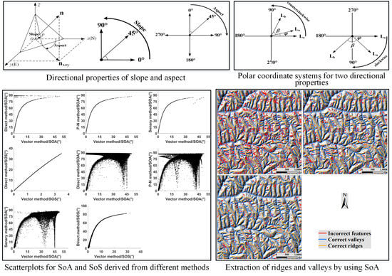
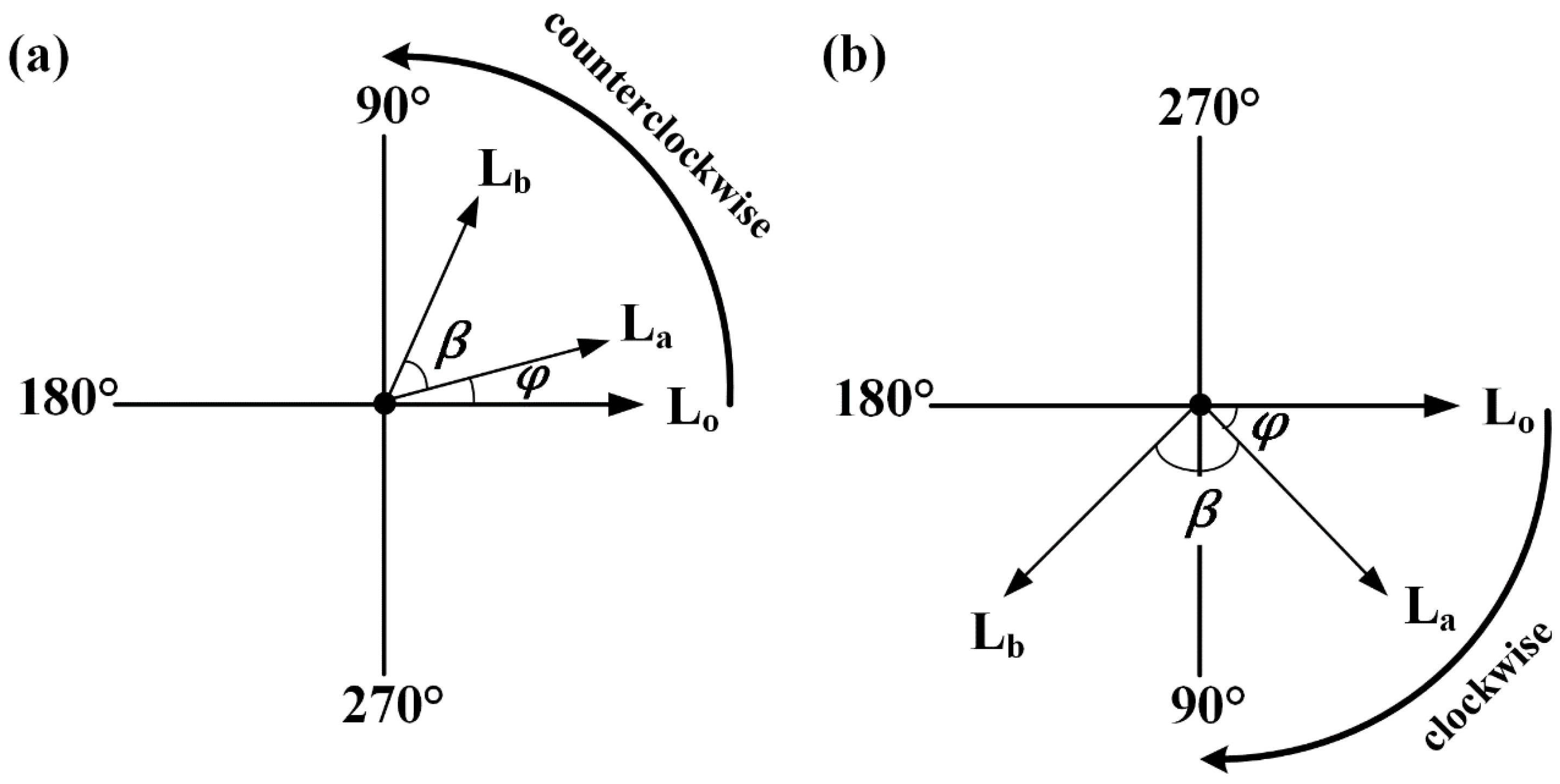
  • Rotation-type judgment. Two rotation types, namely, counterclockwise (slope) and clockwise (aspect), can be observed in the directional property of first-order terrain derivatives (Figure 1). In the counterclockwise or clockwise systems, initial direction, end direction, and rotation angle consist of the aforementioned systems. These systems follow the characteristics of a polar coordinate system (Figure 2). Given the differences between counterclockwise and clockwise systems, a standard polar coordinate system corresponds to a counterclockwise directional property of first-order terrain derivatives, i.e., slope as an example in Figure 2a. By contrast, a reverse polar coordinate system corresponds to a clockwise directional property of first-order terrain derivatives, i.e., aspect as an example in Figure 2b. The initial direction of the polar coordinate system is Lo, which is also the initial direction of the reverse polar coordinate system.
  • Standardization of initial direction. The initial direction of a polar coordinate system faces east, and the initial direction of several first-order terrain derivatives faces other directions, e.g., the initial direction of aspect faces north (Figure 1c). Thus, the initial direction must be standardized before calculating the vector operation of second-order terrain derivatives. For a first-order terrain derivative, its initial direction can be the same as that of the polar coordinate system, i.e., the initial direction of slope also faces east (Figure 2a). However, the angle can be 270° of the initial direction, which faces north in the polar coordinate system, i.e., aspect in Figure 2b. Thus, the initial direction of first-order terrain derivatives is defined as La, and the initial direction of the polar coordinate system is defined as Lo. The angle difference between the two initial directions should be a variable, which is defined as φ. Thus, for any direction of the first-order terrain derivative matrix, i.e., β, which is the angle between the initial direction (La) and the actual direction (Lb), the new direction (θ) of the first-order terrain derivatives in the polar coordinate system can be calculated using the following equation:
    θ = { φ + β , 0 < φ + β < 360 φ + β 360 , φ + β > 360
    where φ is the constant angle from Lo to La, β is the actual angle of the terrain derivative, and θ is the angle of the new direction in the polar coordinate system.
  • Vector representation. These angles can be expressed as vectors in their respective polar coordinate systems based on the transformed directional property in the polar coordinate system.
    A = ( r , θ )
    where r is the length, which should be the cell size of raster data; and θ is the transformed directions in the polar coordinate system. However, if the polar coordinate system is a reverse system, then this system should be further transformed into a standard system using following equation:
    A = ( r , 360 θ )
Lastly, the vector of first-order terrain derivatives can be represented as plane coordinates. The conversion equation is as follows:
{ x = r cos α y = r sin α
where r is the cell size of the raster, and α is the angle of vector A. The derivative in the plane rectangular coordinate system is finally expressed as vector A = (x, y).

2.3. Vectorization Expression of First-Order Terrain Derivatives

In a plane coordinate system, the operation algorithm between vectors is as follows.
When a = ( x 1 , y 1 ) and b = ( x 2 , y 2 ) , then a ± b = ( x 1 ± x 2 , y 1 ± y 2 ) .
When a = ( x , y ) and the real number is λ, then λ a = ( λ x , λ y ) .
When a = ( x , y ) , the length of a is | a | = x 2 + y 2 .
In terms of the third-order finite difference algorithm for calculating second-order terrain derivatives, the preceding vector operations can be performed to implement this algorithm. On the basis of the slope calculation method and Equations (1) and (6) can be derived to calculate second-order terrain derivatives as follows:
2 n d o r d e r = arctan v x 2 + v y 2 × 180 π
where vx and vy are vector changes of the derivatives on a surface point in its neighboring E–W and N–S directions, respectively.

3. Case Study Areas and Data

In this work, four different types of case study areas are selected to validate the proposed vector method: simulated mathematical Gaussian surface, loess landform area, structural landform area, and karst landform area. The proposed vector operation method is applied to the four case study areas to extract second-order terrain derivatives. Among these areas, the Gaussian surface is a simulated mathematical terrain surface defined by Equation (7) [30] as follows:
z = A [ 1 ( x m ) 2 ] e ( x m ) 2 ( y n + 1 ) 2 C e ( x m + 1 ) 2 ( y n ) 2 B [ 0.2 ( x m ) ( x m ) 3 ( y n ) 5 ] e ( x m ) 2 ( y n ) 2
where A, B, and C are terrain relief parameters; and m and n are range control parameters. The mathematical equation can build a series of DEMs and calculate their partial derivatives, which are then used to calculate the first-order terrain derivatives of slope and aspect. The calculated slope and aspect are further used to extract the second-order terrain derivatives of SoS and SoA. In this research, the aforementioned parameters are set as follows: A = 500, B = 1800, C = 1/500, m = 500, and n = 500. These parameter values help produce a typical mathematical Gaussian surface with relatively large elevation and slope differences [30]. The standard deviation of z is 9.20, the average value of z is 122.38, and the grid resolution is 5 m. Lastly, a mathematical terrain surface can be constructed as shown in Figure 3. Considering that the arrows are too dense for the 5 m resolution data, the sample interval is set as 20 m to draw the Gaussian surface with normal vectors in Figure 3. The normal vector of each grid point on the surface can be obtained using the equation. Figure 3b–d show the vector field and its partially enlarged illustrations.
The locations of the loess, structural, and karst landform study areas are presented in Figure 4. The two neighboring loess landforms are located in Suide County (TA1 and TA2 in Figure 4), a typical loess hilly–gully landform [31]. The structural landform is located in Mount Lu (TA3 in Figure 4), which is characterized by rich structural features. The karst landform is located in Dahua, (TA4 in Figure 4), where the topographical features consist of many complex Fenglin and Fengcong units [32]. Given their complex topographical features, the three landform areas exhibit gradual-, sudden-, and non-changing surface morphologies. Thus, second-order terrain derivatives (i.e., SoS and SoA) can improve the understanding of the topographical environment in these areas. The basic information of the three areas is provided in Table 1. DEM data with 5 m and 1 m cell sizes from these areas are used as basic elevation data to calculate second-order derivatives. The DEM data, interpolated from contour topographic maps, in the three areas with cell sizes of 5 m are used as the basic elevation data. Moreover, the DEM data with 1 m resolution is obtained from the UAV Photogrammetry. In addition, these 5 m DEM data are resampled into 10, 15, 20, 25, and 30 m DEM data to investigate the scale effect and the capability of the proposed method using the nearest neighbor method. Moreover, the 1 m DEM data is also resampled into 2, 4, 8, 16, and 32 m (i.e., geometric progressions) DEM data to further investigate the scale effect.

4. Results

In this study, partial derivatives (i.e., fx and fy) are first calculated from the different case study areas. Then, the first-order terrain derivatives of aspect and slope are calculated in these areas. Lastly, the second-order terrain derivatives of SoA and SoS are extracted using the proposed vector operation method. This method is also compared with traditional scalar operation methods for SoA (i.e., direct, P–N, and senary methods).

4.1. SoA and SoS of the Gaussian Surface

For the Gaussian surface, Figure 5 shows the SoA results of the vector method (Figure 5d) and the traditional scalar methods (Figure 5a–c). An evident phenomenon of “north error” (i.e., the four red lines with extremely high SoA value) occurs in the result of the direct method (Figure 5a). By contrast, the P–N and senary methods improve this “north error.” In addition, slight differences can be observed between the results of the P–N (Figure 5b) and senary (Figure 5c) methods [33]. However, the result of the proposed vector method considerably differs from those of the traditional scalar methods. In general, surface morphology consists of gradual-, sudden-, and non-changing characteristics. From the perspective of surface morphology composition, the morphologies of gradual- and non-changing areas should occupy most parts of the terrain, and the morphologies of sudden changing areas should be represented by topographical skeletons or geomorphological boundaries (e.g., ridges, valleys, and slope toes). These topographical skeletons provide high-frequency information of the topography although they only occupy a small portion. The frequency distribution of SoA calculated using different methods is also shown in Figure 6a. The SoA results are normalized (by using min-max normalization method) to display the trends of all the methods. The frequency distribution shows that the curves of the scalar methods (direct, senary, and P–N methods) exhibit profound similarities. By contrast, the curve of the vector method extremely differs from those of the others. This difference shows that the frequency distribution of the vector method appears more suitable for gradual-, sudden-, and non-changing terrain compositions. However, other large SoA values occur in the traditional scalar methods. This frequency distribution difference is further investigated in the landform areas to check the capability of our proposed method.
The direct and vector methods are also used to calculate SoS on the Gaussian surface, and the result is presented in Figure 5e,f. The difference in visual effects between the results of the direct method (Figure 5e) and the vector method (Figure 5f) appears minimal. Furthermore, the frequency distribution curves of the two results are shown in Figure 6b. In general, a DEM with a smooth surface can be derived from a mathematical Gaussian equation. In contrast with the aspect result, the calculated slope should consist of more gradual- and non-changing areas with this smooth DEM. In this scenario, the curves of the two methods are normally similar to that of the smooth mathematical Gaussian surface.

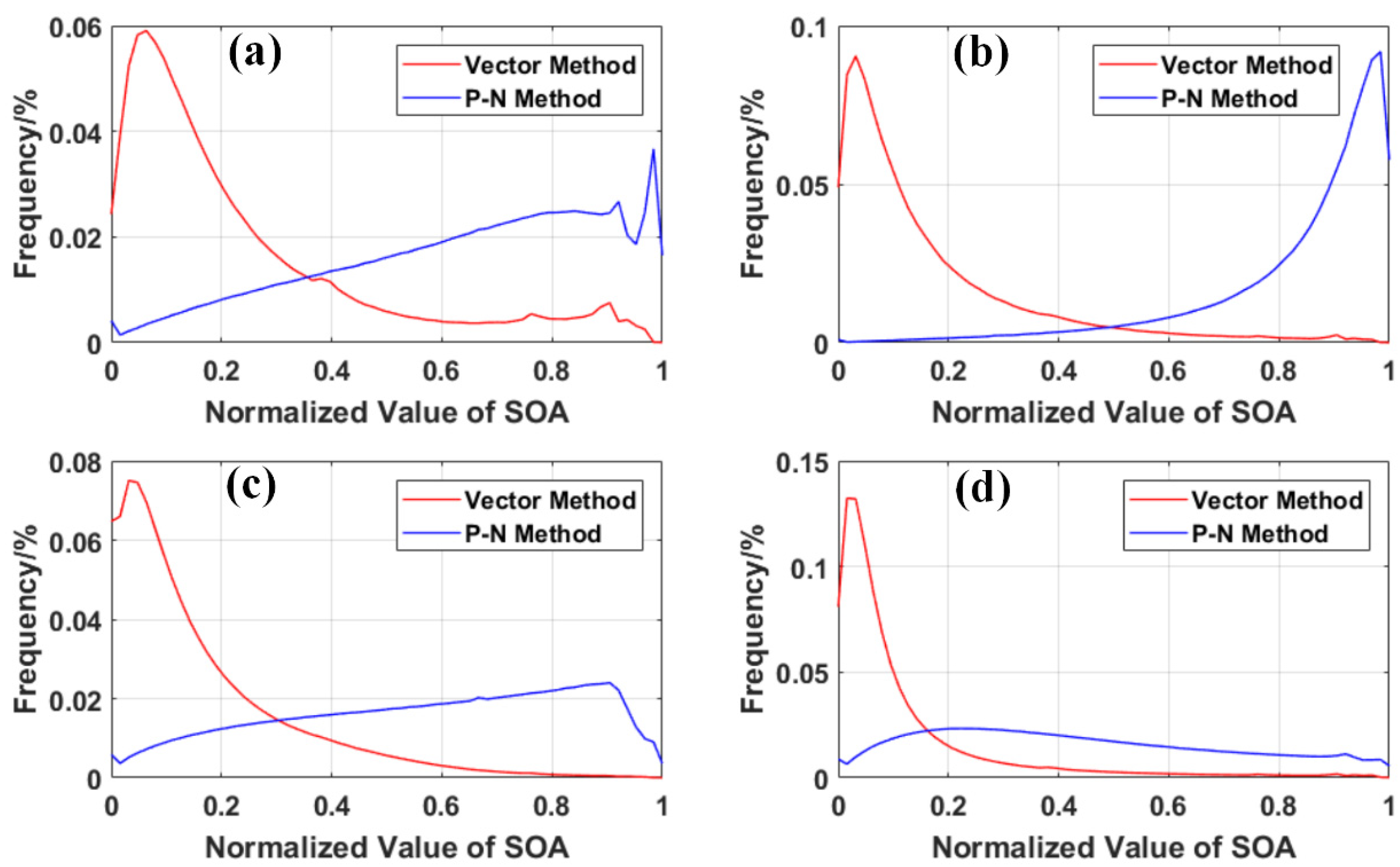
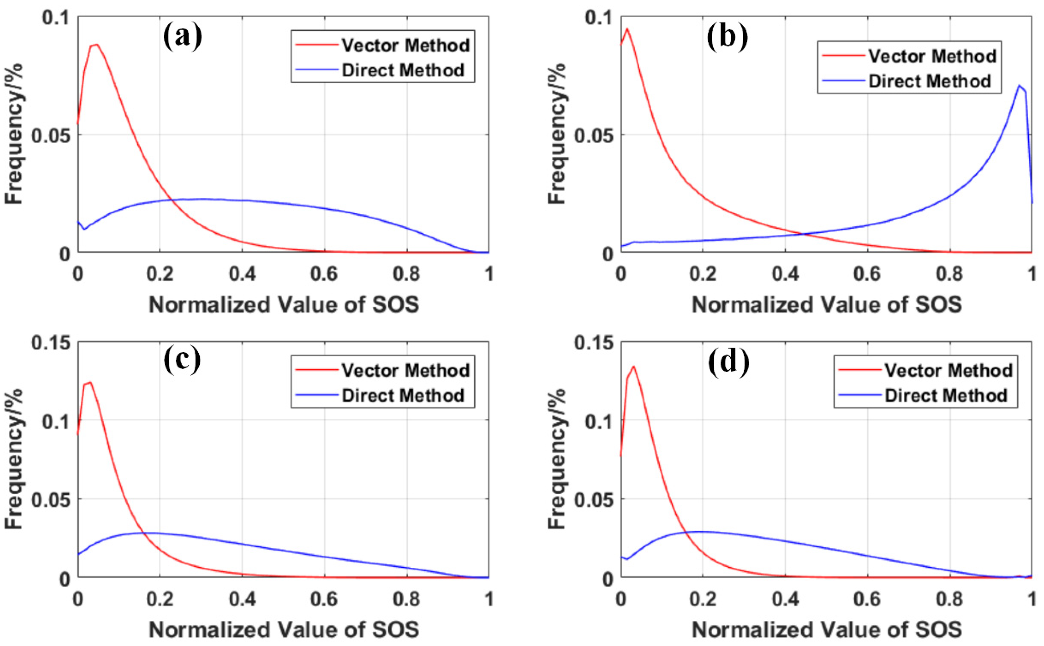
4.2. SoA and SoS of Different Landform Areas

A slight difference is observed among the results of traditional scalar methods of SoA on the Gaussian surface (Figure 6a). Thus, the P–N and proposed vector methods are further applied to different landform areas. Using the 5 m cell size DEM data, the results of the two methods in Suide TA1, Mount Lu, and Dahua areas are presented in Figure 7. In addition, the results for the 1 m cell size data in Suide TA2 are also shown in Figure 7. The results of the vector method are overlaid with hill shadings to enhance their appearance. As indicated by the two calculated SoA results in the different landform areas, the results of the vector method differ considerably from that of the traditional scalar method, thereby drawing a similar conclusion from the result of the Gaussian surface. In the results of the vector method, the terrain features with high SoA values exhibit the strong spatial structure of the terrain skeleton. Meanwhile, the low SoA areas should belong to the surface morphology of gradual- and non-changing areas (Figure 7b,e,h,k). However, the traditional scalar method disregards the directional property of aspect, thereby leading to an overexpression or even exaggeration of the aspect change calculation (i.e., SoA). Such overexpression further causes a misunderstanding regarding the surface morphology compositions of sudden-, gradual-, and non-changing terrain structures. The SoS results are also explored between traditional scalar and vector method in the three different landform areas. The results of the landform areas differ considerably from those of the Gaussian surface. The results of the vector method are also overlaid with hill shadings to enhance their appearance (Figure 8). The visual effects between the direct and vector methods exhibit apparent differences among the three landforms. The spatial structure from the vector method should be clearer than that from the direct method in areas with high SoS values. In these areas, the change in slope is high with complex terrain situations, such as steep cliffs, ridges, and terraces.
In contrast with the smooth Gaussian surface, the terrain morphology of the different landform areas appears complex and consists of many details. By using the 1 m and 5 m cell size DEM data, detailed information of aspect change can be clearly expressed. The frequency distribution curves of the P–N and vector methods in the Suide, Mount Lu, and Dahua areas are shown in Figure 9a–d. From Figure 7 and Figure 9, terrain features (e.g., ridges, valleys, slope toes) clearly occupy a small part of the area. However, these parts should be regarded as key positions of topography, which function as the terrain skeleton of a landform. A relatively large value of SoA areas should normally be located in terrain skeletons, which correspond to a sudden-changing area with a considerable aspect change. The frequency distribution curves of SoS are also shown in Figure 10a–d. With the understanding of the compositions of non-, gradual-, and sudden-changing surface morphologies in mountainous areas, the SoS distribution from the vector method also appears suitable. The frequency curves of SoA and SoS obtained using the vector method show that the low values of SoA and SoS account for the majority. Conversely, the high values of SoA and SoS comprise a small proportion. Evidently, this result follows the natural cognition and understanding of the aspect change phenomenon and surface morphology composition in mountainous areas. By contrast, the frequency curves of SoA obtained using the P–N method and SoS obtained using the direct method show that the frequency of large values for SoA and SoS is considerably higher than that of small values. This result implies that the aspect and slope change information is overexpressed and exaggerated by the scalar method to a considerable extent.

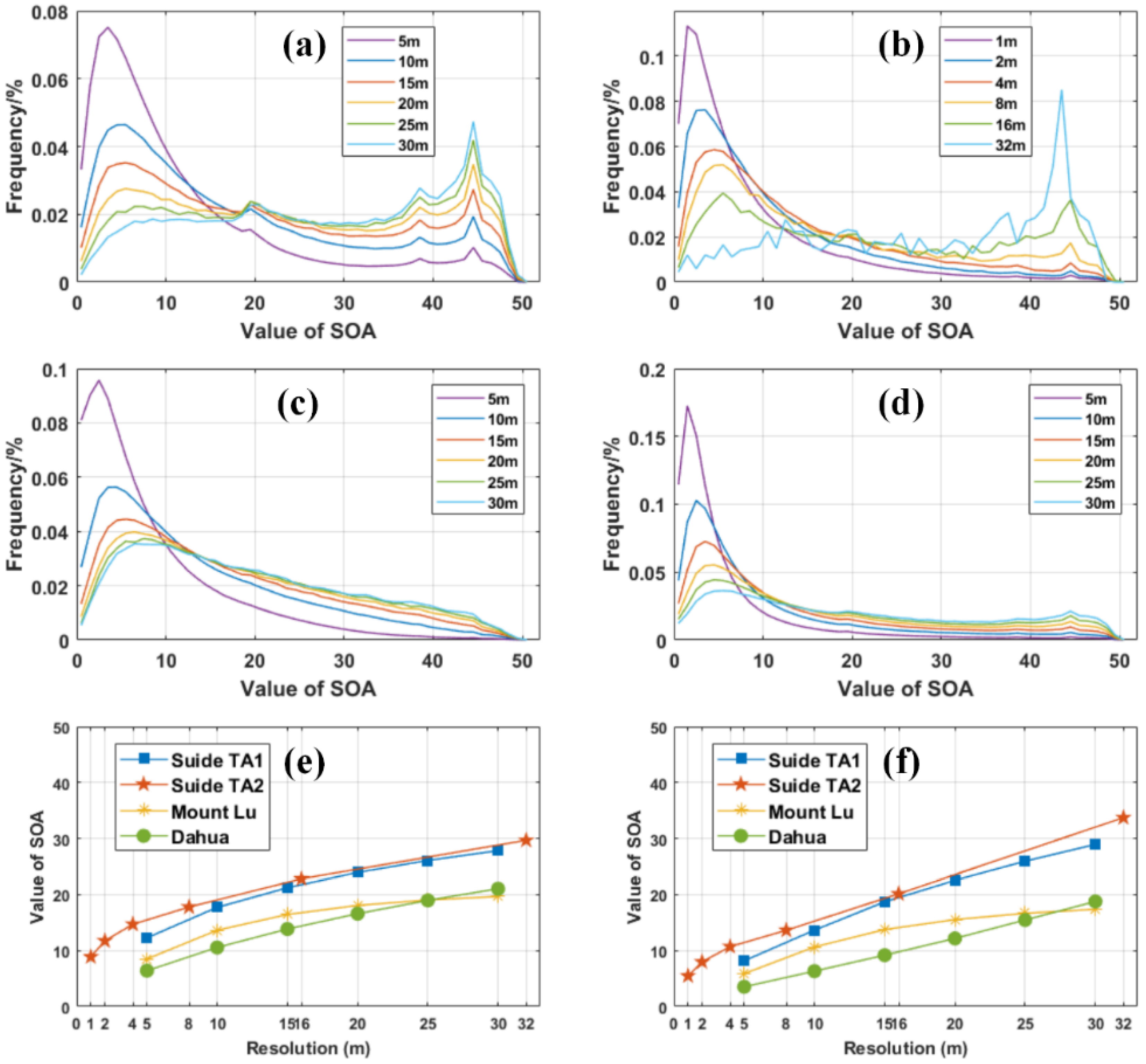
4.3. Assessment of DEM Resolution Effects

In the digital terrain analysis, significant scale effects can be observed from varied DEM cell sizes on the calculated terrain derivatives [34]. This scale effect was also investigated using the proposed vector operation method. Using the resampled 5 m DEM data with resolutions of 10, 15, 20, 25, and 30 m, and 1 m DEM data with resolutions of 2, 4, 8, 16, and 32 m, the proposed vector operation method was further applied to calculate SoA and SoS. Using the vector method, the frequency distribution curves, mean, and median of SoA and SoS in DEMs with different resolutions are shown in Figure 11 and Figure 12.
Using the 5 m and 1 m resolution DEMs, the detailed terrain information can be expressed in the four sample areas; thus, the characteristics of the surface morphology of non- and gradual-changing areas can be accurately expressed [35]. However, as cell size increases, the information of several low-level valleys, ridges, steep cliffs, steep ridges, and terraces can be integrated. In such a situation, high-level terrain features are still preserved, and the total number of cells decreases with the resampling process. Thus, the proportion of terrain features with high SoA and SoS values should be increased (Figure 11a–d and Figure 12a–d). In addition, the SoA and SoS results appear to initially increase slightly and then gradually remain stable with an increase in DEM cell size. That is, DEM cell size exerts limited effect on the SoA and SoS results of the proposed vector method, thereby demonstrating the capability of this method.

5. Discussion

5.1. Correlation among Different Methods

Figure 13a–c show the nonlinear correlation between the scalar and vector methods for SoA in the mathematical Gaussian surface. Specifically, each subfigure indicates that the direct method of SoA generates many high-value pixels (Figure 13a). On the contrary, the senary method produces relatively low-value pixels (approximately 40° of the vector method for SoA) (Figure 13c). Furthermore, the results of the scalar and vector methods for SoS have strong linear correlation (Figure 13d).
In real landform Suide TA1, the direct method of SoA also generates numerous high-value pixels (Figure 13e). Unlike the Gaussian surface, the P-N method of SoA still leaves many high-value pixels in the real landform (Figure 13b–f). Meanwhile, the senary method can improve these high values (Figure 13g). A mass of strange points exists around 45° of the SoA in the vector method. The extraction of the SoA value around 45° is displayed (i.e., from 30° to 46°) in Figure 13i. These areas are terrain features (ridges and valleys), indicating that although these areas should have high values, the scalar methods for SoA produce many low values in the terrain feature areas. Furthermore, the correlation between the direct and vector methods for SoS (Figure 13h) is non-linear in the real landform, which is different from that in the the Gaussian surface. This phenomenon can be attributed to complex terrain morphology of the real landform, which is unlike that of the mathematical surface.

5.2. Comparison of the Vector and Scalar Methods in Terrain Feature Extraction

Terrain feature extraction is an important step in geomorphological recognition and ecological modeling [36,37]. Terrain features determine the basic surface morphology (i.e., ridges and valleys) of landforms. The hydrological analysis method has been extensively used to extract ridges and valleys in loess landforms because of its relative accuracy. However, many areas in the valley portion can be manually modified due to the depression filling process [38]. This modification can lead to an inaccurate valley area, although a continuous steam network can be achieved [39]. In addition, this hydrological method cannot be applied to karst and interior drainage areas [40]. Conversely, natural valleys and ridges can be extracted easily using our proposed method. Multiple levels of ridges and valleys can be extracted conveniently by adjusting the thresholds of SoA.
Using 5 m cell size DEM data, the SoA calculated by the vector method is applied to extract the terrain features of valleys and ridges in the Suide area [11]. In accordance with the range of SoA and its frequency distribution, thresholds of 12, 20, and 25 are used to extract valleys and ridges. Different details of terrain features can be extracted with varying thresholds of SoA (Figure 14). Low-level ridges and valleys can be detected in the low threshold. However, these features can be disregarded by the traditional hydrological method. By contrast, high-level ridges and valleys still exist in the high threshold. Precision (also known as producer’s accuracy), recall (also known as user’s accuracy), and F-measure are widely used for accuracy assessment. Details about these indices can be obtained from the cited works [41,42,43]. The reference data of ridges and valleys in Suide is generated by the visual interpretation of hill shading and images. Table 2 shows the accuracy with different SoA thresholds in Suide. As the SoA threshold increases, the precision increased persistently, whereas the recall decreased because of missing real terrain features. This experiment also shows a good capacity of noise reducing of the vector operation method. The SoA based on the vector method exhibits accuracy and applicability in extracting terrain features, which has a reference value on geomorphological mapping. The vector method is also compared with the traditional scalar direct method to explore its capability. By adjusting the thresholds of the results of the direct and vector methods, the ridges and valleys are extracted. The Figure 15 shows that the north errors clearly exist in the result of the direct method. These north errors cannot be removed by increasing the threshold of SoA based on the direct method.

5.3. Implications of the Vector Method for Other Terrain Derivative Calculation

This research proposes and applies a vector method to calculate second-order terrain derivatives while considering the directional property of first-order terrain derivatives. The first-order terrain derivatives of slope and aspect clearly exhibit a directional property. Given this directional property, the vector operation method should be reliable when calculating their second-order terrain derivatives. Although only two terrain derivatives (e.g., slope and aspect) are tested in this study, the calculation of other terrain derivatives (i.e., any first-order, second-order, or Nth-order terrain derivatives) can be processed using the vector method. To a certain extent, Earth is modeled and expressed in a 3D coordinate system. When using this coordinate system, all geomorphological attributes (e.g., elevation) are implied to have the directional properties of X, Y, and Z. Thus, the vector operation method for calculating terrain derivatives should be more reasonable than traditional scalar operation methods.
In addition, apart from considering a 3D coordinate system with the directional property of coordinates, the calculation of terrain derivatives should be processed using the vector operation method. This suggestion is based on several terrain derivatives with a clear directional property, whereas other derivatives exhibit only a connotative directional property. For example, the terrain derivative of slope length, whose calculation is a top–down cumulative process, should be considered a connotative directional property [44] The terrain derivative of flow direction is referred to as a certain clear direction, which is typically used as a preprocess for flow accumulation. Thus, scalar operation methods that are extensively used in digital terrain analysis require urgent improvement. When attention is focused on the spatial change rules of terrain derivatives with a connotative directional property, the vector operation method should be more reasonable. In summary, we preliminarily explore the calculation of second-order terrain derivatives using the concept of a vector operation method. This concept and method can be applied to calculating other terrain derivatives in geomorphometry.

6. Conclusions

Considering the directional property, a vector operation method is proposed to calculate second-order terrain derivatives. The directional property is considered and vectorized through the following steps: rotation-type judgment, standardization of initial direction, and vector representation. Presenting the first-order terrain derivatives of slope and aspect as examples, their second-order terrain derivatives are calculated using the proposed vector method. The calculated second-order terrain derivatives should be reasonable and accurate, thereby serving as effective expressions and characterizations of surface morphology.
The calculated second-order terrain derivatives demonstrate that the proposed vector method can avoid the errors of overexpression or even exaggeration effectively compared with the scalar methods. The frequency distribution of the second-order terrain derivatives (i.e., SoS and SoA) obtained using the vector method is suitable for gradual-, sudden-, and non-changing terrain compositions. The proposed method can also maintain the stability of the calculated second-order terrain derivatives with different DEM data cell sizes. Lastly, the concept of the vector operation method can be expanded and applied in calculating other terrain derivatives during the terrain analysis process.
In existing geomorphometry theories and methods, scalar operation methods are widely used in terrain derivative calculation. However, some terrain derivatives exhibit the directional property. Thus, scalar methods may lead to calculation errors and a misunderstanding of these terrain derivatives. In this study, we preliminarily explore the calculation of second-order terrain derivatives using the vector operation concept. This concept and its corresponding method should be further explored because they are expected to create a new potential research direction in digital terrain analysis. In addition, neighborhood analysis with different algebraic operations should be a common approach in GIScience research. However, the original vector or raster data for such neighborhood analysis may exhibit a clear or connotative directional property. This directional property should be concerned in algebraic operation processes. Thus, the vector operation method should be promoted in GIScience.

Author Contributions

G.H. proposed the method, performed analysis and wrote the paper. L.X. conceived the study and designed the experiments. W.D. collected and processed the data. S.L. was responsible for the conceptualization, review and editing of this paper. G.T. provided the funding for this research. All authors have read and agreed to the published version of the manuscript.

Funding

This research has been supported by the National Natural Science Foundation of China (No. 41930102, No. 41971333).

Acknowledgments

The codes and the Gaussian surface DEM data that support the findings of this study are available in the “GitHub” repository through the public link https://github.com/NJNU-DTA/second-order_terrain_derivatives. The ground high-resolution DEM data were provided by the Chinese government. The authors do not have the right to make them publicly available on the Internet. However, these data can be used in the authors’ lab. In addition, other DEM data can be used to test the proposed vector method.

Conflicts of Interest

The authors declare no conflict of interest.

Appendix A

Xie et al. argued that the SoA (i.e., angle change) between two slope aspects should not exceed 180°, and the range of the SoA between two aspects is [0°, 180°] [24]. However, the angle change of the two aspects may be outside of the reasonable range in the traditional SoA calculation method because the range of the aspect value is [0°, 360°). The “north error” is a special case because the angle change approaches the maximum value. Thus, Xie et al. proposed the senary method to calculate the SoA. The third-order finite difference method is used to calculate the change rate of the aspect values [24].
{ f x = ( z i + 1 , j 1 z i 1 , j 1 ) + 2 ( z i + 1 , j z i 1 , j ) + ( z i + 1 , j + 1 z i 1 , j + 1 ) 8 g f y = ( z i + 1 , j + 1 z i + 1 , j 1 ) + 2 ( z i , j + 1 z i , j 1 ) + ( z i 1 , j + 1 z i 1 , j 1 ) 8 g
where z represents the aspect value on a grid cell; i and j represent the row and column of the grid cell, respectively; and g represents the grid cell size. Before calculating fx and fy, Equation (1) should be disassembled to Equation (A2).
f x 1 = z i + 1 , j 1 z i 1 , j 1 f y 1 = z i + 1 , j + 1 z i + 1 , j 1 f x 2 = z i + 1 , j z i 1 , j f y 2 = z i , j + 1 z i , j 1 f x 3 = z i + 1 , j + 1 z i 1 , j + 1 f y 3 = z i 1 , j + 1 z i 1 , j 1
The six aforementioned equations are the sub equations (i.e., the senary method) of Equation (A1). Then, the Equation (A1) can be transformed into:
{ f x = f x 1 + 2 f x 2 + f x 3 8 g f y = f y 1 + 2 f y 2 + f y 3 8 g
Thus, the key of the calculation is to ensure that the results of fxi and fyi (i = 1, 2, 3) are correct in Equation (A3). The six parameters (i.e., fxi and fyi (i = 1, 2, 3)) can be corrected with the transformation of the slope aspect value using Equation (A4) as follows.
d i f f _ r { d i f f 360 d i f f d i f f + 360 d i f f ( 180 , 360 ) d i f f ( 180 , 180 ) d i f f ( 360 , 180 )
where diff is the original angle difference between the two aspect fields (i.e., fxi and fyi (i = 1, 2, 3)), and diff_r is the corrected angle difference. After the processing by Equation (A4), Equation (A3) will be transformed into Equation (A5).
{ f x = f x 1 + 2 f x 2 + f x 3 8 g f y = f y 1 + 2 f y 2 + f y 3 8 g
where f’xi and f’yi (i = 1, 2, 3) are derived from fxi and fyi (i = 1, 2, 3) by using Equation (A4). Finally, the SoA can be calculated using Equation (A6) as follows:
S o A = arctan ( ( f x ) 2 + ( f y ) 2 ) 180 π
The flow chart of this method is presented below.
Figure A1. Flowchart of the senary method for calculating SoA [24].
Remotesensing 12 03134 g0a1

References

  1. Florinsky, I.V. Digital Terrain Analysis in Soil Science and Geology; Academic Press: Cambridge, MA, USA, 2016. [Google Scholar]
  2. Wilson, J.P. Environmental Applications of Digital Terrain Modeling; John Wiley & Sons: Hoboken, NJ, USA, 2018. [Google Scholar]
  3. Xiong, L.-Y.; Tang, G.-A.; Zhu, A.-X.; Qian, Y.-Q. A peak-cluster assessment method for the identification of upland planation surfaces. Int. J. Geogr. Inf. Sci. 2017, 31, 387–404. [Google Scholar] [CrossRef]
  4. Florinsky, I.V. An illustrated introduction to general geomorphometry. Prog. Phys. Geogr. 2017, 41, 723–752. [Google Scholar] [CrossRef]
  5. Evans, I.S. Geomorphometry and landform mapping: What is a landform? Geomorphology 2012, 137, 94–106. [Google Scholar] [CrossRef]
  6. Gumindoga, W.; Rwasoka, D.; Murwira, A. Simulation of streamflow using TOPMODEL in the Upper Save River catchment of Zimbabwe. Phys. Chem. Earth Parts A/B/C 2011, 36, 806–813. [Google Scholar] [CrossRef]
  7. Callow, J.N.; Van Niel, K.P.; Boggs, G.S. How does modifying a DEM to reflect known hydrology affect subsequent terrain analysis? J. Hydrol. 2007, 332, 30–39. [Google Scholar] [CrossRef]
  8. Xiong, L.Y.; Tang, G.A.; Strobl, J.; Zhu, A.X. Paleotopographic controls on loess deposition in the Loess Plateau of China. Earth Surf. Proc. Land. 2016, 41, 1155–1168. [Google Scholar] [CrossRef]
  9. Minár, J.; Jenčo, M.; Evans, I.S.; Minár, J., Jr.; Kadlec, M.; Krcho, J.; Pacina, J.; Burian, L.; Benová, A. Third-order geomorphometric variables (derivatives): Definition, computation and utilization of changes of curvatures. Int. J. Geogr. Inf. Sci. 2013, 27, 1381–1402. [Google Scholar] [CrossRef]
  10. Song, X.; Tang, G.; Li, F.; Jiang, L.; Zhou, Y.; Qian, K. Extraction of loess shoulder-line based on the parallel GVF snake model in the loess hilly area of China. Comput. Geosci. 2013, 52, 11–20. [Google Scholar] [CrossRef]
  11. Zhou, Y.; Zhao, H.; Chen, M.; Tu, J.; Yan, L. Automatic detection of lunar craters based on DEM data with the terrain analysis method. Planet. Space Sci. 2018, 160, 1–11. [Google Scholar] [CrossRef]
  12. Ruiz-Arias, J.; Tovar-Pescador, J.; Pozo-Vázquez, D.; Alsamamra, H. A comparative analysis of DEM-based models to estimate the solar radiation in mountainous terrain. Int. J. Geogr. Inf. Sci. 2009, 23, 1049–1076. [Google Scholar] [CrossRef]
  13. Shary, P.A.; Sharaya, L.S.; Mitusov, A.V. Fundamental quantitative methods of land surface analysis. Geoderma 2002, 107, 1–32. [Google Scholar] [CrossRef]
  14. Schmidt, J.; Evans, I.S.; Brinkmann, J. Comparison of polynomial models for land surface curvature calculation. Int. J. Geogr. Inf. Sci. 2003, 17, 797–814. [Google Scholar] [CrossRef]
  15. Florinsky, I.V. Accuracy of local topographic variables derived from digital elevation models. Int. J. Geogr. Inf. Sci. 1998, 12, 47–62. [Google Scholar] [CrossRef]
  16. Wilson, J.P. Geomorphometry: Today and Tomorrow. PeerJ Prepr. 2018, 6, e27197v27191. [Google Scholar] [CrossRef]
  17. Hodgson, M.E.; Gaile, G.L. Characteric mean and dispersion in surface orientations for a zone. Int. J. Geogr. Inf. Syst. 1996, 10, 817–830. [Google Scholar] [CrossRef]
  18. Li, X.; Hodgson, M.E. Vector field data model and operations. GISci. Remote Sens. 2004, 41, 1–24. [Google Scholar] [CrossRef]
  19. Tang, G. A Research on the Accuracy of Digital Elevation Models; Science Press: Beijing, China, 2000. [Google Scholar]
  20. Cheng, G.; Liu, L.; Jing, N.; Chen, L.; Xiong, W. General-purpose optimization methods for parallelization of digital terrain analysis based on cellular automata. Comput. Geosci. 2012, 45, 57–67. [Google Scholar] [CrossRef]
  21. Cao, M.; Tang, G.; Zhang, F.; Yang, J. A cellular automata model for simulating the evolution of positive–negative terrains in a small loess watershed. Int. J. Geogr. Inf. Sci. 2013, 27, 1349–1363. [Google Scholar] [CrossRef]
  22. Shen, Q.; Wang, Y.; Wang, X.; Liu, X.; Zhang, X.; Zhang, S. Comparing interpolation methods to predict soil total phosphorus in the Mollisol area of Northeast China. Catena 2019, 174, 59–72. [Google Scholar] [CrossRef]
  23. Hu, Q.; Zhou, Y.; Wang, S.; Wang, F. Machine learning and fractal theory models for landslide susceptibility mapping: Case study from the Jinsha River Basin. Geomorphology 2020, 351, 106975. [Google Scholar] [CrossRef]
  24. Xie, Y.; Tang, G.; Jiang, L. Characteristics and correcting methods of errors in extraction of SOA based on DEMs. Geogr. Geo Inf. Sci. 2013, 29, 49–53. (In Chinese) [Google Scholar]
  25. She, J.; Li, X. Map algebra based analysis for directed flow networks. Trans. GIS 2016, 20, 356–367. [Google Scholar] [CrossRef]
  26. Ritter, P. A vector-based slope and aspect generation algorithm. Photogr. Eng. Remote Sens. 1987, 53, 1109–1111. [Google Scholar]
  27. Horn, B.K. Hill shading and the reflectance map. Proc. IEEE 1981, 69, 14–47. [Google Scholar] [CrossRef] [Green Version]
  28. Skidmore, A.K. A comparison of techniques for calculating gradient and aspect from a gridded digital elevation model. Int. J. Geogr. Inf. Syst. 1989, 3, 323–334. [Google Scholar] [CrossRef]
  29. Bolstad, P.V.; Stowe, T. An evaluation of DEM accuracy: Elevation, slope, and aspect. Photogr. Eng. Remote Sens. 1994, 60, 1327–1332. [Google Scholar]
  30. Zhou, Q.; Liu, X. Analysis of errors of derived slope and aspect related to DEM data properties. Comput. Geosci. 2004, 30, 369–378. [Google Scholar] [CrossRef]
  31. Xiong, L.-Y.; Tang, G.-A.; Zhu, A.-X.; Li, J.-L.; Duan, J.-Z.; Qian, Y.-Q. Landform-derived placement of electrical resistivity prospecting for paleotopography reconstruction in the loess landforms of China. J. Appl. Geophys. 2016, 131, 1–13. [Google Scholar] [CrossRef]
  32. Yang, X.; Tang, G.; Meng, X.; Xiong, L. Classification of Karst Fenglin and Fengcong Landform Units Based on Spatial Relations of Terrain Feature Points from DEMs. Remote Sens. 2019, 11, 1950. [Google Scholar] [CrossRef] [Green Version]
  33. Hu, G.; Xiong, L.; Tang, G. Vector geometry based method for the extraction of slope of aspect by using DEMs. Acta Geod. Cartogr. Sin. 2019, 48, 1404–1414. [Google Scholar] [CrossRef]
  34. Goodchild, M.F. Scale in GIS: An overview. Geomorphology 2011, 130, 5–9. [Google Scholar] [CrossRef]
  35. Dai, W.; Yang, X.; Na, J.; Li, J.; Brus, D.; Xiong, L.; Tang, G.; Huang, X. Effects of DEM resolution on the accuracy of gully maps in loess hilly areas. Catena 2019, 177, 114–125. [Google Scholar] [CrossRef]
  36. Tien Bui, D.; Shirzadi, A.; Shahabi, H.; Chapi, K.; Omidavr, E.; Pham, B.T.; Talebpour Asl, D.; Khaledian, H.; Pradhan, B.; Panahi, M.; et al. A Novel Ensemble Artificial Intelligence Approach for Gully Erosion Mapping in a Semi-Arid Watershed (Iran). Sensors 2019, 19, 2444. [Google Scholar] [CrossRef] [Green Version]
  37. Li, S.; Xiong, L.; Tang, G.; Strobl, J. Deep learning-based approach for landform classification from integrated data sources of digital elevation model and imagery. Geomorphology 2020, 354, 107045. [Google Scholar] [CrossRef]
  38. Xiong, L.Y.; Jiang, R.Q.; Lu, Q.H.; Yang, B.S.; Li, F.Y.; Tang, G.A. Improved Priority-Flood method for depression filling by redundant calculation optimization in local micro-relief areas. Trans. GIS 2019, 23, 259–274. [Google Scholar] [CrossRef]
  39. Byun, J.; Seong, Y.B. An algorithm to extract more accurate stream longitudinal profiles from unfilled DEMs. Geomorphology 2015, 242, 38–48. [Google Scholar] [CrossRef]
  40. Dorsaz, J.M.; Gironás, J.; Escauriaza, C.; Rinaldo, A. The geomorphometry of endorheic drainage basins: Implications for interpreting and modelling their evolution. Earth Surf. Proc. Landf. 2013, 38, 1881–1896. [Google Scholar] [CrossRef]
  41. Dai, W.; Na, J.; Huang, N.; Hu, G.; Yang, X.; Tang, G.; Xiong, L.; Li, F. Integrated edge detection and terrain analysis for agricultural terrace delineation from remote sensing images. Int. J. Geogr. Inf. Sci. 2020, 34, 484–503. [Google Scholar] [CrossRef]
  42. Dai, W.; Hu, G.; Huang, N.; Zhang, P.; Yang, X.; Tang, G. A Contour-Directional Detection for Deriving Terrace Ridge From Open Source Images and Digital Elevation Models. IEEE Access 2019, 7, 129215–129224. [Google Scholar] [CrossRef]
  43. Dai, W.; Hu, G.; Yang, X.; Yang, X.W.; Cheng, Y.; Xiong, L.; Strobl, J.; Tang, G. Identifying ephemeral gullies from high-resolution images and DEMs using flow-directional detection. J. Mt. Sci. 2020. accepted. [Google Scholar] [CrossRef]
  44. Hickey, R. Slope angle and slope length solutions for GIS. Cartography 2000, 29, 1–8. [Google Scholar] [CrossRef]
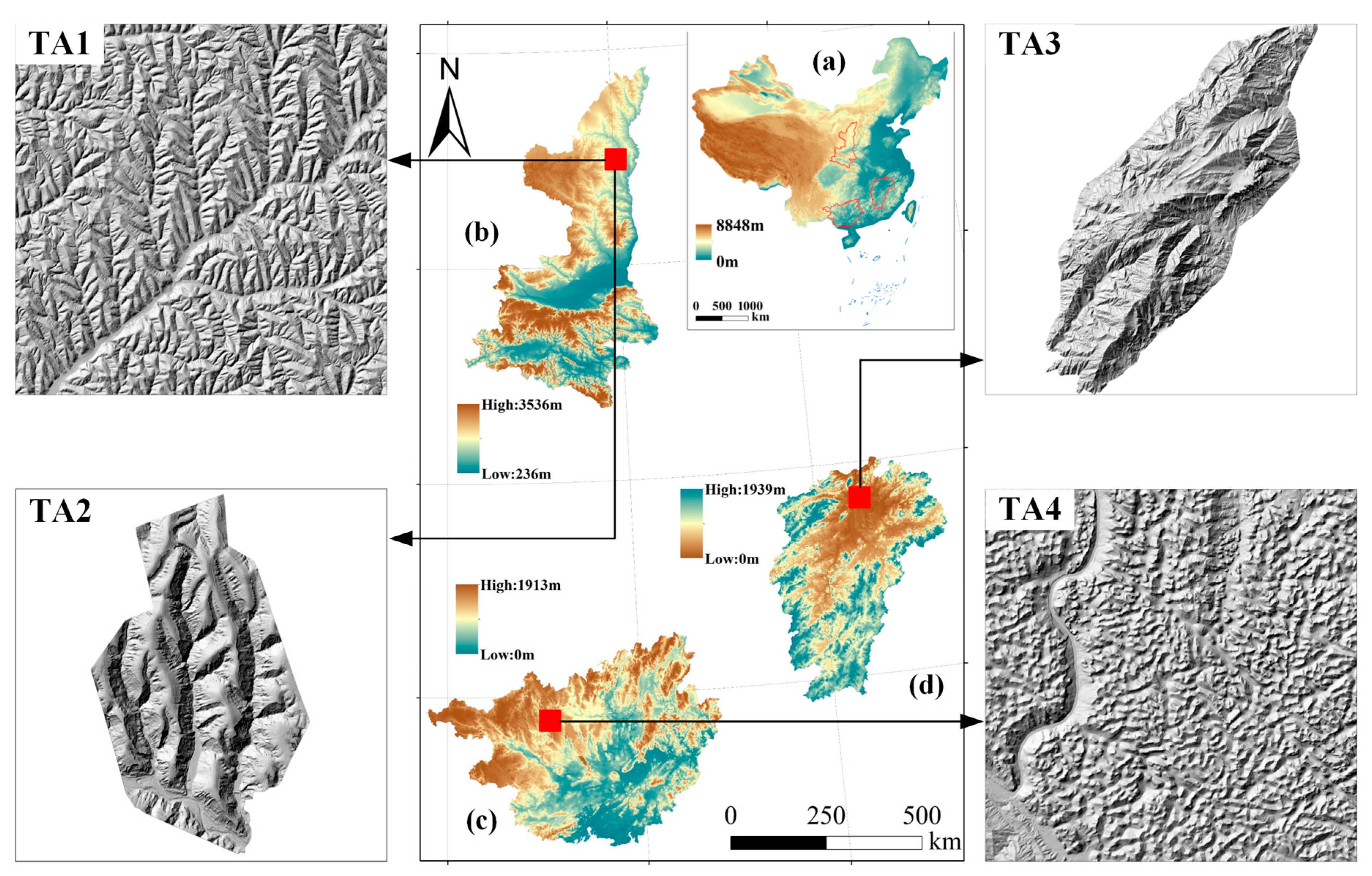
Figure 1. Directional properties of several basic terrain derivatives and scalar and vector operations. (a) is the calculation principle of slope and aspect on surface point p; (b) represents the directional property of slope from the horizontal direction to the zenith direction (counterclockwise); (c) denotes the directional property of aspect from the north, to the east, south, west, and back to the north (clockwise); (d) is a scalar operation; and (e) is a vector operation.
Remotesensing 12 03134 g001
Figure 2. Polar coordinate systems for the counterclockwise and clockwise directional properties. (a) Standard and (b) reverse polar coordinate systems.
Remotesensing 12 03134 g002
Figure 3. Simulated Gaussian surface (a) and its normal vector field in different parts (bd).
Remotesensing 12 03134 g003
Figure 4. Ground study areas. (a) Study areas in China, (b) Suide area (TA1 and TA2) in Shaanxi Province, (c) Dahua area (TA4) in Guangxi Province, and (d) Mount Lu area (TA3) in Jiangxi Province.
Remotesensing 12 03134 g004
Figure 5. Slope of aspect (SoA) and slope of slope (SoS) results for the Gaussian surface using different methods. (a) Direct, (b) P–N, (c) senary, and (d) vector methods for SoA. (e) Direct and (f) vector methods for SoS. The unit is degree.
Remotesensing 12 03134 g005
Figure 6. Frequency distribution using different methods on the Gaussian surface. Curves of (a) SoA and (b) SoS.
Remotesensing 12 03134 g006
Figure 7. SoA results of different methods in different areas. (a) P–N and (b) vector methods in Suide TA1, (c) vector method with hill shading in Suide TA1, (d) P–N and (e) vector methods in Suide TA2, (f) vector method with hill shading in Suide TA2, (g) P–N and (h) vector methods in Mount Lu, (i) vector method with hill shading in Mount Lu, (j) P–N and (k) vector methods in Dahua, (l) vector method with hill shading in Dahua. The unit is degree.
Remotesensing 12 03134 g007
Figure 8. SoS results of different methods in different areas. (a) Direct and (b) vector methods in Suide TA1, (c) vector method with hill shading in Suide TA1, (d) direct and (e) vector methods in Suide TA2, (f) vector method with hill shading in Suide TA2, (g) direct and (h) vector methods in Mount Lu, (i) vector method with hill shading in Mount Lu, (j) direct and (k) vector methods in Dahua, (l) vector method with hill shading in Dahua. The unit is degree.
Remotesensing 12 03134 g008
Figure 9. Frequency distribution of SoA using different methods in different areas. (a) Suide TA1, (b) Suide TA2, (c) Mount Lu, and (d) Dahua.
Remotesensing 12 03134 g009
Figure 10. Frequency distribution of SoS using different methods in different areas. (a) Suide TA1, (b) Suide TA2, (c) Mount Lu, and (d) Dahua.
Remotesensing 12 03134 g010
Figure 11. Statistics of the SoA results based on different resolutions using the vector method in different areas. (a) Suide TA1, (b) Suide TA2, (c) Mount Lu, (d) Dahua, (e) mean values, and (f) median values.
Remotesensing 12 03134 g011
Figure 12. Statistics of the SoS results based on different resolutions using the vector method in different areas. (a) Suide TA1, (b) Suide TA2, (c) Mount Lu, (d) Dahua, (e) mean values, and (f) median values.
Remotesensing 12 03134 g012
Figure 13. Scatterplots for SoA and SoS derived from different methods on Gaussian surface and real landform Suide TA1. Gaussian surface: SoA calculated by the (a) direct, (b) P-N, and (c) senary methods; SoS calculated by the (d) direct method. Real landform Suide TA1: SoA calculated by the (e) direct, (f) P–N, and (g) senary methods; SoS calculated by the (h) direct method. All these methods are compared with the vector method. Extractions (i) (red color) of range [30°, 46°] for SoA in Suide TA1.
Remotesensing 12 03134 g013
Figure 14. Extraction of ridges and valleys with different thresholds using the SoA derived from the vector method in Suide TA1. The thresholds are (a) 15, (b) 20, and (c) 25.
Remotesensing 12 03134 g014
Figure 15. Extraction of ridges and valleys using the SoA derived from the direct and vector methods. Ridge extraction using the (a) vector and (b) direct methods and (c) the stacked results of both methods. Valley extraction using the (d) vector and (e) direct methods and (f) the stacked results of both methods.
Remotesensing 12 03134 g015
Table 1. Basic information of the three landform areas.
Sample
Areas
Elevation
(m)
Average
Height (m)
SD
Height (m)
Average
Slope (°)
Min–Max
Slope (°)
SD
Slope (°)
Area
(km2)
Landform
Type
TA1814–1188996.967.7829.280–82.883.4197.15Loess landform
TA2784–987883.067.0332.970–83.044.211.92Loess landform
TA389–1470710.3317.9231.580–86.943.52180.43Structural landform
TA4166–1163821.4512.8729.700–89.413.69361.19Karst landform
Table 2. Accuracy of terrain feature lines with different SoA thresholds in Suide.
SoA ThresholdLcLeLrPrecisionRecallF-Measure
15182,000.77326,021.61182,971.3755.82%99.47%71.51%
20178,168.25247,039.42182,971.3772.12%97.37%82.87%
25173,473.66205,916.77182,971.3784.24%94.81%89.22%
Lc is the total length of correctly identified terrain feature lines, Le indicates the total length of all extracted terrain feature lines, including correct and incorrect detections, and Lr is the total length of reference terrain feature lines. Their unit is meter (m).

