Mud Volcanism at the Taman Peninsula: Multiscale Analysis of Remote Sensing and Morphometric Data


Abstract
:
1. Introduction
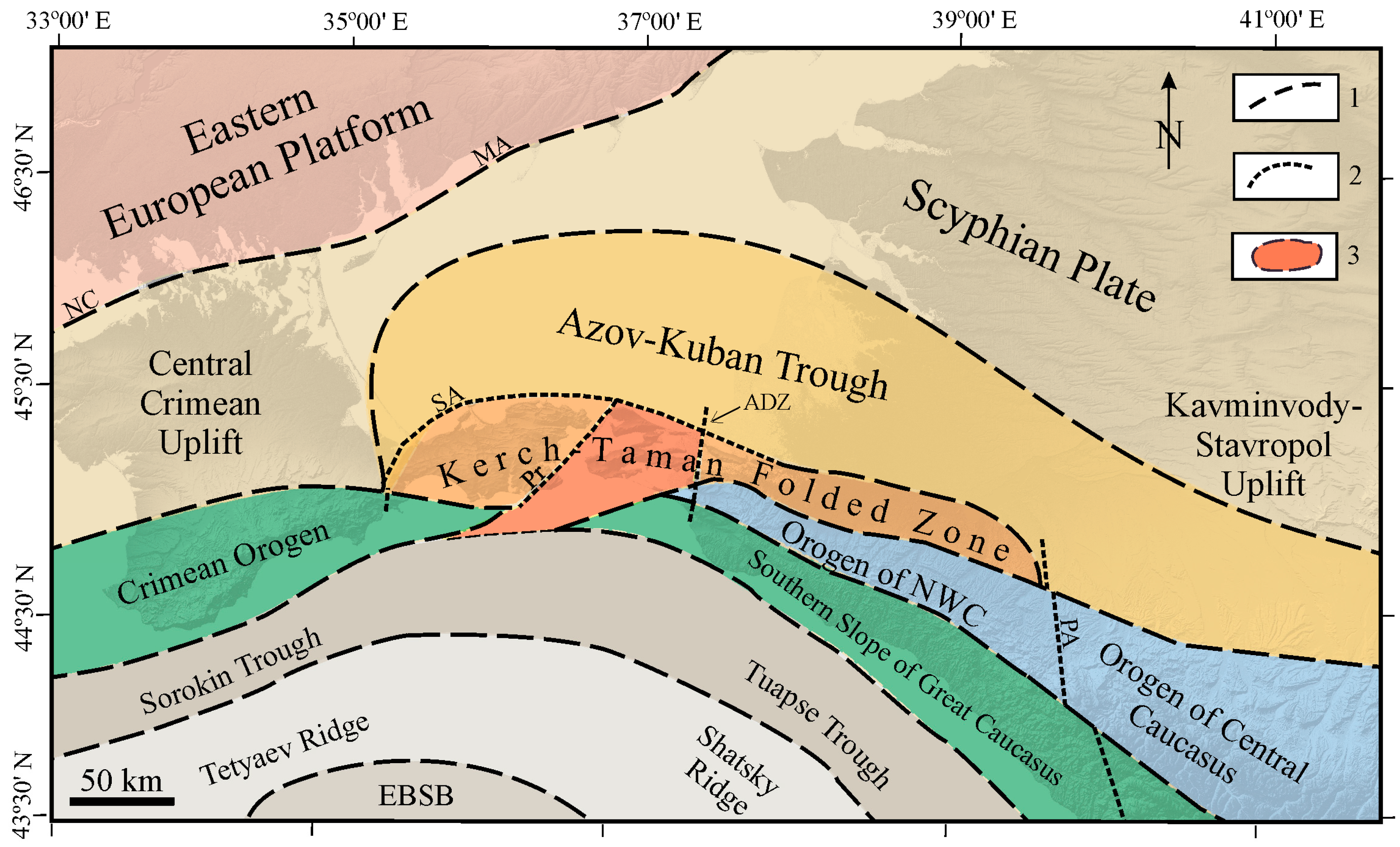
2. Study Area
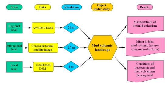
3. Materials and Methods
3.1. Regional Level
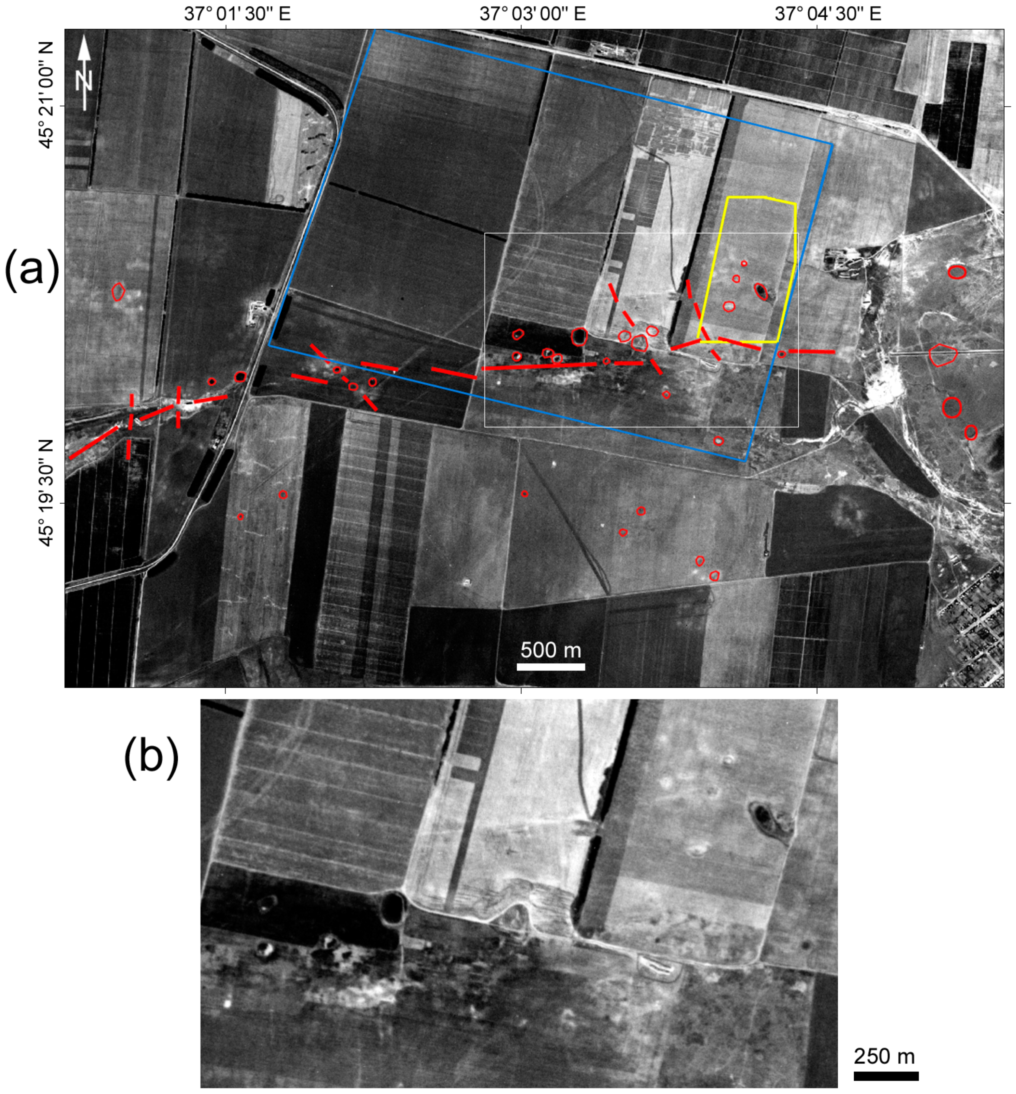
3.2. Subregional Level
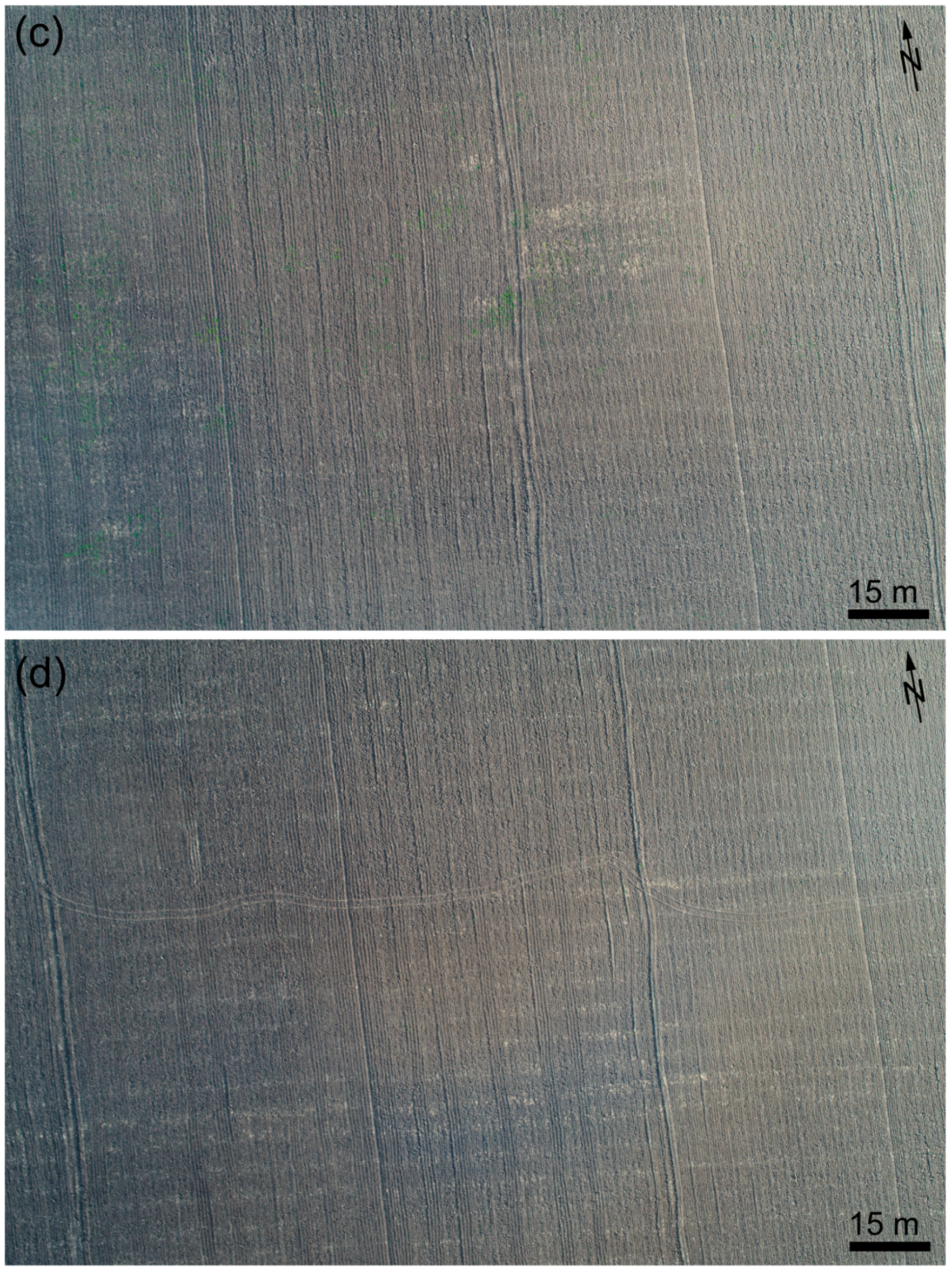
3.3. Local Level
3.3.1. Field Works
3.3.2. Data Processing
- Aligning aerial images by the least-squares bundle adjustment with data from the camera self- calibration based on the GCP coordinates. The planimetric and vertical root mean square errors (RMSEs) of the aerial triangulation were 0.5 cm and 2.5 cm, correspondingly.
- Generating a 1-m gridded DSM by the inverse distance weighted interpolation [53] of the dense point cloud.
- Producing an orthomosaic with a resolution of 0.2 m.
3.3.3. Geomorphometric Modeling
3.4. GIS-Based Analysis
4. Results
5. Discussion
6. Conclusions
Author Contributions
Funding
Conflicts of Interest
References
- Dimitrov, I.L. Mud volcanoes—The most important pathway for degassing deeply buried sediments. Earth Sci. Rev. 2002, 59, 49–76. [Google Scholar] [CrossRef]
- Kopf, A.J. Significance of mud volcanism. Rev. Geophys. 2002, 40, 1–52. [Google Scholar] [CrossRef] [Green Version]
- Mazzini, A.; Etiope, G. Mud volcanism: An updated review. Earth Sci. Rev. 2017, 168, 81–112. [Google Scholar] [CrossRef] [Green Version]
- Shnyukov, Y.F.; Sheremetyev, V.M.; Maslakov, N.A.; Kutny, V.A.; Gusakov, I.N.; Trofimov, V.V. Mud Volcanoes of the Kerch–Taman Region; GlavMedia: Krasnodar, Russia, 2006; 174p. (In Russian) [Google Scholar]
- Shnyukov, Y.F.; Aliyev, A.A.; Rahmanov, R.R. Mud volcanism of Mediterranean, Black and Caspian seas: Specificity of development and manifestations. Geol. Miner. Resour. World Ocean 2017, 13, 5–25. [Google Scholar] [CrossRef]
- Sobisevich, A.L.; Sobisevich, L.E.; Tveritinova, T.Y. On mud volcanism in the Late Alpine folded edifice of the North-Western Caucasus (Exemplified by the study of the deep structure of the Shugo Mud Volcano). Geol. Miner. Resour. World Ocean 2014, 36, 80–93, (In Russian, with English Abstract). [Google Scholar]
- Tveritinova, T.Y.; Sobisevich, A.L.; Sobisevich, L.E.; Likhodeev, D.V. Structural position and structure peculiarities of the Mount Karabetov Mud Volcano. Geol. Miner. Resour. World Ocean 2015, 40, 106–122, (In Russian, with English Abstract). [Google Scholar]
- Podymov, I.S. A map of mud volcanoes of the Taman Peninsula. In Research and Monitoring of Mud Volcanism of Taman in the Context of the Modern Problem of Ecological Safety for the Azov-Black Sea Coast of Russia; Southern Branch, Shirshov Institute of Oceanology, Russian Academy of Science: Gelendzhik, Russia, 2015; Available online: https://mud-volcano.coastdyn.ru/map.html (accessed on 6 November 2020). (In Russian)
- Trifonov, V.G.; Makarov, V.I.; Safonov, Y.G.; Florensky, P.V. (Eds.) Space Remote Sensing Data in Geology; Nauka: Moscow, Russia, 1983; 535p, (In Russian, with English Contents). [Google Scholar]
- Scanvic, J.-Y. Aerospatial Remote Sensing in Geology; Balkema: Rotterdam, The Netherlands, 1997; 280p. [Google Scholar]
- Gupta, R.P. Remote Sensing Geology, 2nd ed.; Springer: Berlin, Germany, 2003; 655p. [Google Scholar]
- Florinsky, I.V. Digital Terrain Analysis in Soil Science and Geology; Elsevier: Amsterdam, The Netherlands, 2016; p. 486. [Google Scholar]
- Colomina, I.; Molina, P. Unmanned aerial systems for photogrammetry and remote sensing: A review. ISPRS J. Photogramm. Remote Sens. 2014, 92, 79–97. [Google Scholar] [CrossRef] [Green Version]
- Shahbazi, M.; Théau, J.; Menard, P. Recent applications of unmanned aerial imagery in natural resource management. GISci. Remote Sens. 2014, 51, 339–365. [Google Scholar] [CrossRef]
- Whitehead, K.; Hugenholtz, C.H. Remote sensing of the environment with small unmanned aircraft systems (UASs), part 1: A review of progress and challenges. J. Unmanned Veh. Syst. 2014, 2, 69–85. [Google Scholar] [CrossRef]
- Whitehead, K.; Hugenholtz, C.H.; Myshak, S.; Brown, O.; LeClair, A.; Tamminga, A.; Barchyn, T.E.; Moorman, B.; Eaton, B. Remote sensing of the environment with small unmanned aircraft systems (UASs), part 2: Scientific and commercial applications. J. Unmanned Veh. Syst. 2014, 2, 86–102. [Google Scholar] [CrossRef] [Green Version]
- Pajares, G. Overview and current status of remote sensing applications based on unmanned aerial vehicles (UAVs). Photogramm. Eng. Remote Sens. 2015, 81, 281–330. [Google Scholar] [CrossRef] [Green Version]
- Bhardwaj, A.; Sam, L.; Akanksha; Martín-Torres, F.J.; Kumar, R. UAVs as remote sensing platform in glaciology: Present applications and future prospects. Remote Sens. Environ. 2016, 175, 196–204. [Google Scholar] [CrossRef]
- Toth, C.K.; Jóźków, G. Remote sensing platforms and sensors: A survey. ISPRS J. Photogramm. Remote Sens. 2016, 115, 22–36. [Google Scholar] [CrossRef]
- Woodget, A.S.; Austrums, R.; Maddock, I.P.; Habit, E. Drones and digital photogrammetry: From classifications to continuums for monitoring river habitat and hydromorphology. Wiley Interdiscip. Rev. Water 2017, 4, e1222. [Google Scholar] [CrossRef] [Green Version]
- Singh, K.K.; Frazier, A.E. A meta-analysis and review of unmanned aircraft system (UAS) imagery for terrestrial applications. Int. J. Remote Sens. 2018, 39, 5078–5098. [Google Scholar] [CrossRef]
- Xiang, T.-Z.; Xia, G.-S.; Zhang, L. Mini-unmanned aerial vehicle-based remote sensing: Techniques, applications, and prospects. IEEE Geosci. Remote Sens. Mag. 2019, 7, 29–63. [Google Scholar] [CrossRef] [Green Version]
- Santagata, T. Monitoring of the Nirano Mud Volcanoes Regional Natural Reserve (North Italy) using unmanned aerial vehicles and terrestrial laser scanning. J. Imaging 2017, 3, 42. [Google Scholar] [CrossRef] [Green Version]
- Di Felice, F.; Mazzini, A.; Di Stefano, G.; Romeo, G. Drone high resolution infrared imaging of the Lusi mud eruption. Mar. Pet. Geol. 2018, 90, 38–51. [Google Scholar] [CrossRef]
- Di Stefano, G.; Romeo, G.; Mazzini, A.; Iarocci, A.; Hadi, S.; Pelphrey, S. The Lusi drone: A multidisciplinary tool to access extreme environments. Mar. Pet. Geol. 2018, 90, 26–37. [Google Scholar] [CrossRef]
- Blagovolin, N.S. Geomorphology of the Kerch–Taman Region; Soviet Academic Press: Moscow, Russia, 1962; 201p. (In Russian) [Google Scholar]
- Gaydalenok, O.V. Structure of the Kerch-Taman Zone of Folded Deformations of the Azov-Kuban Trough. Ph.D. Thesis, Geological Institute, Russian Academy of Sciences, Moscow, Russia, 2020; 128p. (In Russian). [Google Scholar]
- Trifonov, V.G.; Sokolov, S.Y.; Sokolov, S.A.; Hessami, K. Mesozoic–Cenozoic Structure of the Black Sea–Caucasus–Caspian Region and Its Relationships with the Upper Mantle Structure. Geotectonics 2020, 54, 331–355. [Google Scholar] [CrossRef]
- Tadono, T.; Nagai, H.; Ishida, H.; Oda, F.; Naito, S.; Minakawa, K.; Iwamoto, H. generation of the 30 m-mesh global digital surface model by ALOS PRISM. ISPRS Int. Arch. Photogramm. Remote Sens. Spat. Inf. Sci. 2016, 41, 157–162. [Google Scholar] [CrossRef]
- Florinsky, I.V.; Skrypitsyna, T.N.; Luschikova, O.S. Comparative accuracy of the AW3D30 DSM, ASTER GDEM, and SRTM1 DEM: A case study on the Zaoksky Testing Ground, Central European Russia. Remote Sens. Lett. 2018, 9, 706–714. [Google Scholar] [CrossRef]
- Pavlova, A.I.; Pavlov, A.V. Analysis of correction methods for digital terrain models based on satellite data. Optoelectron. Instrum. Data Process. 2018, 54, 445–450. [Google Scholar] [CrossRef]
- Florinsky, I.V.; Skrypitsyna, T.N.; Trevisani, S.; Romaikin, S.V. Statistical and visual quality assessment of nearly-global and continental digital elevation models of Trentino, Italy. Remote Sens. Lett. 2019, 10, 726–735. [Google Scholar] [CrossRef]
- ALOS Global Digital Surface Model “ALOS World 3D–30m” (AW3D30). Available online: http://www.eorc.jaxa.jp/ALOS/en/aw3d30/ (accessed on 1 November 2019).
- Horn, B. Hill shading and the reflectance map. Proc. IEEE 1981, 69, 14–47. [Google Scholar] [CrossRef] [Green Version]
- Schowengerdt, R.A.; Glass, C.E. Digitally processed topographic data for regional tectonic evaluations. GSA Bull. 1983, 94, 549–556. [Google Scholar] [CrossRef]
- Chorowicz, J.; Dhont, D.; Gündoğdu, N. Neotectonics in the eastern North Anatolian fault region (Turkey) advocates crustal extension: Mapping from SAR ERS imagery and digital elevation model. J. Struct. Geol. 1999, 21, 511–532. [Google Scholar] [CrossRef]
- Earth Resources Observation and Science (EROS) Center. Declassified Satellite Imagery—1; U.S. Geological Survey: Sioux Fall, SD, USA, 1995. [CrossRef]
- Kraus, K. Photogrammetry: Geometry from Images and Laser Scans, 2nd ed.; de Gruyter: Berlin, Germany, 2007; 459p. [Google Scholar]
- Casana, J.; Cothren, J. Stereo analysis, DEM extraction and orthorectification of Corona satellite imagery: Archaeological applications from the Near East. Antiquity 2008, 82, 732–749. [Google Scholar] [CrossRef] [Green Version]
- Kurkov, V.M.; Skripitsina, T.N.; Zhuravlev, D.V.; Schlotzhauer, U.; Kobzev, A.A.; Knyaz, V.A.; Mischka, C. Comprehensive survey of archaeological sites by ground and aerial remote sensing techniques. In Ecology, Economy, Informatics; Matishov, G.G., Ed.; Southern Federal University Publishers: Rostov on Don, Russia, 2018; Volume 3, pp. 151–158, (In Russian, with English Abstract). [Google Scholar] [CrossRef]
- Zhuravlev, D.V.; Batasova, A.V.; Schlotzhauer, U.; Kurkov, V.M.; Skrypitsyna, T.N.; Knyaz, V.A.; Kudryashova, A.I.; Kobzev, A.A.; Mischka, C. New data on the structure of ancient monuments of the Asian Bosporus (from remote sensing data). In XX Bosporan Readings: Cimmerian Bosporus and the World of the Barbarians in Antiquity and the Middle Ages; Main Results and Prospects of Research; Zinko, V.N., Zinko, E.A., Eds.; Vernadsky Crimean Federal University: Simferopol, Russia, 2019; pp. 193–200. (In Russian) [Google Scholar]
- Skrypitsyna, T.N.; Kurkov, V.M.; Kobzev, A.A.; Zhuravlev, D.V. Remote sensing data as a geospatial basis for archaeological research. Eng. Surv. 2019, 13, 18–26. (In Russian) [Google Scholar] [CrossRef]
- Skrypitsyna, T.; Kurkov, V.; Zhuravlev, D.; Knyaz, V.; Batasova, A. Study of the hidden ancient anthropogenic landscapes using digital models of microtopography. Proc. SPIE 2020, 11533, 115331F. [Google Scholar] [CrossRef]
- Verhagen, P.; Drăguţ, L. Object-based landform delineation and classification from DEMs for archaeological predictive mapping. J. Archaeol. Sci. 2012, 39, 698–703. [Google Scholar] [CrossRef]
- Campana, S. Drones in archaeology. State-of-the-art and future perspectives. Archaeol. Prospect. 2017, 24, 275–296. [Google Scholar] [CrossRef]
- Davis, D.S. Object-based image analysis: A review of developments and future directions of automated feature detection in landscape archaeology. Archaeol. Prospect. 2019, 26, 155–163. [Google Scholar] [CrossRef]
- Luo, L.; Wang, X.; Guo, H.; Lasaponara, R.; Zong, X.; Masini, N.; Wang, G.; Shi, P.; Khatteli, H.; Chen, F.; et al. Airborne and spaceborne remote sensing for archaeological and cultural heritage applications: A review of the century (1907–2017). Remote Sens. Environ. 2019, 232, 111280. [Google Scholar] [CrossRef]
- Trebeleva, G.V.; Gorlov, Y.V. Cultural landscape of the Taman Peninsula in ancient times. Reg. Envir. Issues 2019, 1, 39–46, (In Russian, with English Abstract). [Google Scholar] [CrossRef]
- DJI Phantom 4. Available online: https://www.dji.com/phantom-4/info (accessed on 1 November 2019).
- Agisoft LLC. Agisoft PhotoScan User Manual: Professional Edition, Version 1.3; Agisoft LLC: St. Petersburg, Russia, 2017; 105p. [Google Scholar]
- Semenov, A.E.; Kryukov, E.V.; Rykovanov, D.P.; Semenov, D.A. Practical application of computer vision techniques to solve problems of recognition, 3D reconstruction, map stitching, precise targeting, dead reckoning, and navigation. Izv. South. Fed. Univ. Eng. Sci. 2010, 104, 92–102, (In Russian, with English Abstract). [Google Scholar]
- Hirschmuller, H. Stereo processing by semiglobal matching and mutual information. IEEE Trans. Pattern Anal. Mach. Intell. 2008, 30, 328–341. [Google Scholar] [CrossRef]
- Watson, D. Contouring: A Guide to the Analysis and Display of Spatial Data; Pergamon Press: Oxford, UK, 1992; 321p. [Google Scholar]
- Kurkov, V.M.; Kiseleva, A.S. DEM accuracy research based on unmanned aerial survey data. ISPRS Int. Arch. Photogramm. Remote Sens. Spat. Inf. Sci. 2020, XLIII-B3-2020, 1347–1352. [Google Scholar] [CrossRef]
- Shary, P.A.; Sharaya, L.S.; Mitusov, A.V. Fundamental quantitative methods of land surface analysis. Geoderma 2002, 107, 1–32. [Google Scholar] [CrossRef]
- Florinsky, I.V. An illustrated introduction to general geomorphometry. Prog. Phys. Geogr. 2017, 41, 723–752. [Google Scholar] [CrossRef]
- Florinsky, I.V.; Pankratov, A.N. A universal spectral analytical method for digital terrain modeling. Int. J. Geogr. Inf. Sci. 2016, 30, 2506–2528. [Google Scholar] [CrossRef]
- Florinsky, I.V.; Kurkov, V.M.; Bliakharskii, D.P. Geomorphometry from unmanned aerial surveys. Trans. GIS 2017, 22, 58–81. [Google Scholar] [CrossRef]
- Tveritinova, T.Y.; Beloborodov, D.E. Mud volcanoes in the neotectonic structure of the Taman Peninsula. Dyn. Geol. 2020, 2, 157–186. (In Russian) [Google Scholar]
- Trikhunkov, Y.I. Neotectonic transformation of Cenozoic fold structures in the northwestern Caucasus. Geotectonics 2016, 50, 509–521. [Google Scholar] [CrossRef]
- Engibarian, A.A. Lithological, Facies, and Tectonic Criteria for the Oil and Gas Content of the Meso-Cenozoic Deposits of the Taman Peninsula. Ph.D. Thesis, North-Caucasian State Technical University, Stavropol, Russia, 2006; 217p. (In Russian). [Google Scholar]
- Lukina, N.V.; Karakhanyan, A.S.; Senin, B.V.; Skaryatin, V.D.; Trifonov, V.G. Linear and ring structures of the Crimean–Caucasian Region. In Space Remote Sensing Data in Geology; Trifonov, V.G., Makarov, V.I., Safonov, Y.G., Florensky, P.V., Eds.; Nauka: Moscow, Russia, 1983; pp. 195–206. (In Russian) [Google Scholar]
- Tveritinova, T.Y.; Beloborodov, D.E.; Likhodeev, D.V. Mud volcanoes in the structure of the Kerch Peninsula. Dyn. Geol. 2020, 1, 38–54. (In Russian) [Google Scholar]
- Beloborodov, D.E.; Tveritinova, T.Y. Structural position of mud volcanoes in the interpericlinal Kerch-Taman zone. In Fundamental Problems of Tectonics and Geodynamics: Proc. LII Tectonic Meeting; Degtyarev, K.E., Ed.; Geos: Moscow, Russia, 2020; Volume 1, pp. 65–69. (In Russian) [Google Scholar]
- Hengl, T.; Reuter, H.I. (Eds.) Geomorphometry: Concepts, Software, Applications; Elsevier: Amsterdam, The Netherlands, 2009; 796p. [Google Scholar]
- Wilson, J.P. Environmental Applications of Digital Terrain Modeling; Wiley: Hoboken, NJ, USA, 2018; 360p. [Google Scholar]
- Luftwaffe and Allied Aerial Reconnaissance Archives. Research and Digitizing, 2013–2020. Available online: https://www.luftfoto.ru/index.html (accessed on 6 November 2020).


| Variable, Notation, and Unit | Definition, Interpretation, and Formula |
|---|---|
| Slope, G, ° | An angle between the tangential and horizontal planes at a given point of the surface. Relates to the velocity of gravity-driven flows. |
| Minimal curvature, kmin, m−1 | A curvature of a principal section with the lowest value of curvature at a given point of the surface. kmin > 0 corresponds to hills, while kmin < 0 relates to valleys. |
| Maximal curvature, kmax, m−1 | A curvature of a principal section with the highest value of curvature at a given point of the surface. kmax > 0 corresponds to ridges, while kmax < 0 relates to closed depressions. |
| Mean curvature, H, m−1 | A half-sum of curvatures of any two orthogonal normal sections at a given point of the surface. H represents two accumulation mechanisms of gravity-driven substances—convergence and relative deceleration of flows—with equal weights. |
| Gaussian curvature, K, m−2 | A product of maximal and minimal curvatures. K retains values in each point of the surface after its bending without breaking, stretching, and compressing. |
| Unsphericity, M, m−1 | A half-difference of maximal and minimal curvatures. M = 0 on a sphere; M values show the extent to which the shape of the surface is non-spherical at a given point. |
| Horizontal (or tangential) curvature, kh (m−1) | A curvature of a normal section tangential to a contour line at a given point of the surface. kh is a measure of flow convergence and divergence. Gravity-driven lateral flows converge where kh < 0, and diverge where kh > 0. kh reveals ridge and valley spurs. |
| Vertical (or profile) curvature, kv (m−1) | A curvature of a normal section having a common tangent line with a slope line at a given point of the surface. kv is a measure of relative deceleration and acceleration of gravity-driven flows. They are decelerated where kv < 0, and are accelerated where kv > 0. kv mapping allows revealing terraces and scarps. |
| Difference curvature, E, m−1 | A half-difference of vertical and horizontal curvatures. Comparing two accumulation mechanisms of gravity-driven substances, E shows to what extent the relative deceleration of flows is higher than flow convergence at a given point of the surface. |
| Horizontal excess curvature, khe, m−1 | A difference of horizontal and minimal curvatures. khe shows to what extent the bending of a normal section tangential to a contour line is larger than the minimal bending at a given point of the surface. |
| Vertical excess curvature, kve, m−1 | A difference of vertical and minimal curvatures. kve shows to what extent the bending of a normal section having a common tangent line with a slope line is larger than the minimal bending at a given point of the surface. |
| Accumulation curvature, Ka, m−2 | A product of vertical and horizontal curvatures. A measure of the extent of flow accumulation at a given point of the surface. |
| Ring curvature, Kr, m−2 | A product of horizontal excess and vertical excess curvatures. Describes flow line twisting. |
Publisher’s Note: MDPI stays neutral with regard to jurisdictional claims in published maps and institutional affiliations. |
© 2020 by the authors. Licensee MDPI, Basel, Switzerland. This article is an open access article distributed under the terms and conditions of the Creative Commons Attribution (CC BY) license (http://creativecommons.org/licenses/by/4.0/).
Share and Cite
Skrypitsyna, T.N.; Florinsky, I.V.; Beloborodov, D.E.; Gaydalenok, O.V. Mud Volcanism at the Taman Peninsula: Multiscale Analysis of Remote Sensing and Morphometric Data. Remote Sens. 2020, 12, 3763. https://doi.org/10.3390/rs12223763
Skrypitsyna TN, Florinsky IV, Beloborodov DE, Gaydalenok OV. Mud Volcanism at the Taman Peninsula: Multiscale Analysis of Remote Sensing and Morphometric Data. Remote Sensing. 2020; 12(22):3763. https://doi.org/10.3390/rs12223763
Chicago/Turabian StyleSkrypitsyna, Tatyana N., Igor V. Florinsky, Denis E. Beloborodov, and Olga V. Gaydalenok. 2020. "Mud Volcanism at the Taman Peninsula: Multiscale Analysis of Remote Sensing and Morphometric Data" Remote Sensing 12, no. 22: 3763. https://doi.org/10.3390/rs12223763