Abstract
Large-scale multispectral remote sensing data are often unavailable for some practical applications. Spectral resolution enhancement for large-scale multispectral remote sensing images by incorporating small-scale hyperspectral remote sensing images is an alternative way to generate remote sensing images with both large spatial range and high spectral resolution. This paper proposes an improved spectral resolution enhancement method (ISREM) using spectral matrix and weighting the spectral angle of the transformation matrix. ISREM is tested in a typical area of the Three-River Headwaters region (TRHR) to produce a synthetic hyperspectral image (HSI). Two existing spectral resolution enhancement methods, the color resolution improvement software package (CRISP) and spectral resolution enhancement method (SREM), are adopted to compare with ISREM. To further test the practicality of the synthetic HSIs generated by the ISREM, CRISP and SREM, they are used to estimate the coverage of native plant species (NPS) using support vector machines (SVM) and random forest (RF) regressions. The experimental results are as follows. (1) For the Pearson correlation coefficient between the synthetic HSI and original image, ISREM yielded the largest value of 0.9582, followed by CRISP and SREM with values of 0.9480 and 0.9514. For spectral similarity, the HSI generated by the ISREM was the closest to the original reference HSI in the spectral curve. It also showed the best cumulative performance with the use of the three quality evaluation indexes. (2) The identification accuracies of native plant species were 93.51%, 90.91%, 89.61% and 89.61% using generated HSIs and original multispectral image (MSI) within a threshold of 20%, respectively. Compared with original MSI, the synthetic HSI showed better ability to identify NPS in the study area, which further illustrated the effectiveness of the ISREM. (3) The ISREM can reduce the strict requirement of pure pixels and maintain the quality of synthetic HSI by spectral angle weighting. Hence, the proposed ISREM outperforms the existing CRISP and SREM methods in image spectral resolution enhancement of multispectral remote sensing images.
1. Introduction
Spectral enhancement for multispectral remote sensing data greatly improves the utilization efficiency of remote sensing images. The methods for enhancing remote sensing data to study grassland degradation in the TRHR mainly include three groups. (1) The first group of enhancement method for identifying grassland degradation is conducting band math of the remote sensing images, i.e., the vegetation index (VI) and biochemical index. The normalized difference vegetation index (NDVI) is one of the most common spectral enhancement methods for vegetation characterization. The VIs and band math expressions method has been widely used to estimate grassland coverage in the TRHR [1,2]. This kind of method can enhance the recognition ability of remote sensing images through the operation of wave bands, especially the ability to distinguish vegetation from the background. However, due to the limited number of bands, this method is weak for identifying vegetation species. (2) The second group of enhancement methods is image sharpening of HSI to obtain a finer spatial resolution for grassland species identification. The remote sensing image sharpening method generally refers to the fusion of panchromatic images and MSI to enhance the spatial resolution of the MSI [3,4,5]. The enhancement of the spatial resolution of remote sensing data has received considerable attention, but it is rarely applied to grassland vegetation species identification. The most commonly used enhancement method is the classic Gram-Schmidt pan-sharpening method [6]. Gram-Schmidt pan-sharpening is usually used to improve the spatial resolution of HSI with a higher spatial resolution MSI in image preprocessing [7]. Although this method enhances the image recognition ability through an improved spatial resolution, it still has the problem of spectral information distortion, which is not conducive to the recognition of grass species. Through field investigation, we found that various types of grassland in the TRHR were mixed-living together, with low grass height and little difference in morphological characteristics. Thus, the improvement of spatial resolution is of little help for grass species identification; it is more important to improve the spectral resolution to identify grass species of the TRHR. (3) The third group of enhancement methods is spectral enhancement for MSI [8]. A model is first built between the MSI and HSI, and then a synthesized HSI is calculated pixel by pixel or using a fixed size filter [9,10]. This kind of method not only maintains the spatial resolution of MSI but also enhances the spectral resolution of MSI.
Spectral enhancement methods are mainly used to improve the spectral resolution of MSI with an HSI and have great potential in some applications requiring high spectral resolution images. The SREM was first proposed in 2014 and applied in mineral alteration information extraction [11]. However, it has not been applied in vegetation identification or grassland degradation as far as we know. Previous studies of grassland degradation have mainly focused on three aspects: (1) total vegetation or biomass based on a long time series to identify grassland degradation; (2) the use of vegetation indexes, such as VIs and Biological indexes (BIs), to assess grassland coverage; and (3) calculation of net primary productivity and local net primary productivity scaling to monitor grassland degradation [12,13]. However, grassland degradation is not only the degradation of biomass or coverage but also the change in grass species, which is manifested as an increase in noxious weeds (NWs) and a decrease in the dominant native grass species. NWs invasion has become serious in recent years and the extremely degraded black soil has attracted the attention of researchers [11]. The coverage of NPS in the TRHR has been proved to be a decreasing trend in recent decades [14]. Traditional methods have difficulty identifying NPS due to the slight spectral differences between NPS and invasive NWs and the low spectral resolution of MSI for large areas. Thus, specific and effective data that can better distinguish between NPS and invasive NWs should be found and utilized. HSI has been widely applied in mineral resource exploration, inland water remote sensing, and vegetation ecology and agriculture, and has been proven to have a good ability to distinguish between similar spectral features [15]. However, to the best of our knowledge, few studies have used hyperspectral data to identify grass species in the alpine grassland of the TRHR because the temporal and spatial consistency of the samples and images is difficult to achieve.
HSI has sensitive spectral discrimination ability and can be applied to the identification of grassland species to realize the study of grassland degradation in the study area. However, satellite HSI is difficult to apply to the identification of grassland components in large regions due to the small width, low spatial resolution and scarce data source. Therefore, it is of great significance to study methods that can maintain the spectral resolution and expand the spatial coverage of HSI. Due to the important symbiosis of grass species in the study area, it was difficult to find evenly distributed grass species over a large area, and pure pixels were difficult to obtain in the image. Therefore, the SREM method could not be used directly for identifying grass species. Thus, a novel spectral enhancement method based on clustering and spectral angular weight was proposed to improve the spectral resolution of the MSI. Compared with SREM, the proposed ISREM makes two main improvements. (1) MSI were pre-clustered with the clustering method, and the result of the clustering was considered a “pure pixel”, which was used in the calculation. (2) The spectral angle was calculated and used as the weight for each cluster result, and then the spectral value of the predicted pixel was calculated. The detailed implementation of ISREM is described in Section 3.1.
The main contributions of this study are: (1) the proposal of the ISREM for the enhancement of MSI and generation of a synthetic HSI of the study area; (2) features extraction to map the distribution of NPS using the synthetic HSI, and the identification abilities of original MSI and synthetic HSI were compared; and finally, (3) a grassland degradation map was produced based on the distribution map of NPS. As a whole, this study provided a method for identifying the grass types and degradation of plateau grasslands using MSI in the case of HSI absence.
2. Materials and Methods
2.1. Study Area
This study area (Figure 1) is located in the Tongtian River reserve of Yushu Tibetan Autonomous Prefecture, which covers part of southeastern Zhiduo County in Qinghai, China. This area was selected from the hinterland of the TRHR, which is the source region of the Yangtze, Yellow, and Lancang Rivers [11]. The annual average temperature is −0.4°C, with an annual rainfall of ~394 mm/year in the TRHR. The average altitude of the study area is above 4000 m. The climate in this region is dry, cold in winter and cool in summer, with strong solar radiation and thin air. The oxygen content of the air is about 14% in the study area. The cold season lasts nearly 10 months (January–June & September–December), with a large temperature difference between day and night. Approximately 70–90% of the study area is covered by vegetation, and the alpine meadow is the main grassland type in this region [16].
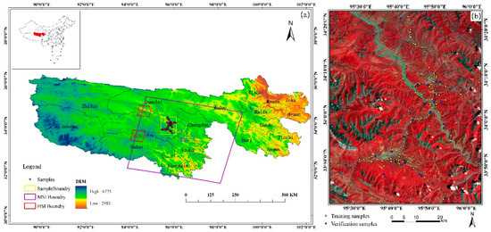
Figure 1.
Location of the study area in the TRHR of the Tibetan Plateau. (a) Location of the TRHR of China with the imagery boundary boxes. (b) False-color image clipped by the sample distribution boundary and synthesized by HJ-1A MSI (band 4, band 3 and band 2).
2.2. Grass Species and Samples Collection
In the study area, the grass species mainly include two kinds of NPS (Kobresia and Stipa capillata) and five kinds of NWs (Leontopodium nanum, Potentilla chinensis Ser, Bryophyte, Polygonum sibiricum Laxm, and Lamiophlomis rotata) [17]. NPS were the native plant community, while NWs have become the secondary vegetation due to overgrazing and climate changes in the TRHR. The invasion of NWs has been accelerating due to their adaptive and reproductive capacity for decades. Because of the pungent taste and toxic of NWs, yak and Tibetan sheep prefer NPS to NWs. In the past, for a long time, the coverage of NPS, suitable for grazing, was decreasing, which is an important indicator of grassland degradation [18]. Therefore, mapping the coverage of NPS is critical for investigating the grassland degradation in the TRHR.
The main objective of the sample collection is to collect the spectra of grasses and samples of grassland coverage. Sampling was carried out from 10 to 19 August 2017 for the first time. The second time, a field survey was conducted from 12 to 23 August 2019. Despite a two-year interval of the two surveys, the changes in spectra and coverage of grass species are negligible [19]. The Grass spectral data were collected using the spectrum-measuring instrument HR-512i, a portable object spectrometer produced by the SVC Company, USA. Spectrum acquisition was performed at 11:00–14:00 on sunny days (Figure 2a). For each kind of grass, at least 10 spectrums were collected from 5 different high-density growing areas and combined to 1 average spectrum. The spectrums of Kobresia, Stipa capillata, Leontopodium nanum, Potentilla chinensis Ser, Bryophyte, Polygonum sibiricum Laxm, and Lamiophlomis rotata were finally generated by SVC HR-512i PC software.
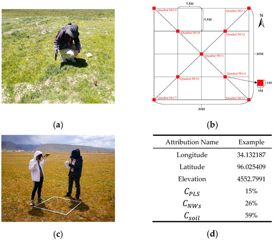
Figure 2.
Sample collection work: (a) Spectrum collection of Stipa capillata; (b) a schematic of “X” sampling method; (c) our team recording the quadrat information; (d) main information attribute table structure of the sample collection at this quadrat.
For the first filed sampling, 113 30 m × 30 m, the same size of the pixel of HJ-1A MSI, grassland coverage samples were collected. A gentle slope and relatively homogeneous of grass species were necessary to select the sampling area. For each 30 m × 30 m sample, nine quadrats with a size of 1 m × 1 m were established and distributed in an “X” shape, with one quadrat at the center and the other eight quadrats in the “X” directions (Figure 2b). Each quadrat unit was comprised of bare soil, PLS and NWs in the research area. The relationship of soil, PLS and NWs can be described as: . is the proportion of soil coverage. respected the proportion of PLS coverage and respected the proportion of NWs. For each quadrat unit, coverage information was recorded as Figure 2d. The location information was acquired from Trimble Geo 7X hand-held submeter GPS units with an accuracy of ~0.5 m in the center of each quadrat. Finally, the average coverage , and of the nine quadrats were calculated, respectively, as the , and values of the 30 m × 30 m sample. The location information of the 30 m × 30 m sample was the same as center quadrat (NO.1 in Figure 2b).
The second sample collection was implemented using the same equipment and methods. A total of 142 new 30 m × 30 m grassland coverage samples were collected in the second survey. Altogether, 255 30 m × 30 m grassland coverage samples were obtained in the study area and used in this paper.
2.3. Image Data Acquisition and Processing
The MSI and HSI used in this paper were provided by the Chinese Environmental Satellite HJ-1A, which is equipped with a CCD camera and an HSI camera. According to the growth period of the vegetation in the study area, one MSI and two HSIs were acquired from the China Centre for Resources Satellite Data and Application (http://www.cresda.com/CN/) on 10 August 2019. The HJ-1A CCD MSI provides 4 visible spectral bands with a spatial resolution of 30 m. The HJ-1A HIS provides 115 bands from 460.04 nm to 951.54 nm with a spatial resolution of 100 m (Table 1).

Table 1.
Comparison between HJ-1A MSI and HSI.
Atmospheric correction for the HJ-1A MSI/HSI 2A class imagery was carried out with the FLASH module in ENVI 5.3. A vertical stripe removal method [20] based on image rotation was utilized to remove the stripe in band 1 to band 25(410 nm to 490 nm). Terrain correction [21] was then carried out using ASTER GDEM in ENVI 5.3. A G-S fusion was used to improve the spatial resolution of HJ-1A HSIs. Finally, HSI and MSI were corrected to the same spatial reference as the sample data.
2.4. Spectral Resolution Enhancement of HJ-1A MSI Imagery
2.4.1. Basic Model
Spectral enhancement of the MSI using HSI should be based on the following assumptions: (1) Because they use the same physical imaging mechanism, both hyperspectral sensors and multispectral sensors have the same spectral response trend in specific wavelengths for imaging the same ground object. (2) The spectral information of ground objects has spatial scale invariance, that is, the spectral characteristics of the same object in different spatial positions are basically the same. (3) The HSI overlaps to some extent with the MSI to be enhanced, and the features in the overlapped region are consistent with the features in the nonoverlapped region to be enhanced [22,23].
MSI and HSI are extensions of two-dimensional images in spectral latitude and can be regarded as three-dimensional images [24]. To facilitate calculation, we converted the three-dimensional images into two-dimensional matrices, each column of which represented pixels, and the rows represented bands. H was assumed to be an HSI with s samples, c columns and k bands. A k × n matrix was converted for H, where N is calculated by s × c. H can be expressed as:
where k represents the band numbers of the HSI and n represents the pixel number in the HSI. H(i) (i is in the range from 1 to N) represents the column vector of the spectral values, and h(i,j) (j is in the range from 1 to k) represents the value of the i-th pixel in the j band. In the same way, the MSI M can be expressed as
where l represents the band numbers of the MSI and N represents the pixel number in the MSI. M(i) (i is in the range from 1 to n) represents the column vector of the spectral values, and m(i,j) (j is in the range from 1 to k) represents the value of the i-th pixel in the j band. For the HSI and MSI in the same space and under the same sensor, MSI can be regarded as the linear representation of HSI [10]. The HSI H is related to the MSI M through the use of a simple filtering matrix F as
where F is a l × k matrix, which is the coefficient of the linear combination of hyperspectral bands into MSI. ε is the Gaussian random error. This inverse process can also be written as
where G is a k × l matrix that also acts to approximately reconstruct the HSI. γ is the Gaussian random error. According to the least square principle, Formula (4) can be used to solve the expression of transformation matrix G for constructing HSI as
To calculate G in (5), there must be more pixels than the number of multispectral bands, which is an easy assumption to satisfy. With a transformation coefficient matrix, the artificial hyperspectral value of the ith pixel is then obtained with the following equation:
where is the ith pixel of the estimated hyperspectral vector and is then combined to construct an estimated HSI as
2.4.2. Clustering for Extraction of Spectral Matrix of HSI and MSI
Theoretically, pure pixels are the most ideal for constructing a transformation matrix G of MSI and HSI. However, limited by the low spatial resolution of the images and irregular distribution of ground objects, endmember extraction of pure pixels is a difficult and complicated task, and the results are easily influenced by the image data [25]. Especially in the grassland area of the plateau, because of the low grassland coverage and mixed grassland communities, it is more difficult to extract pure pixels. Thus, clustering, a less-than-ideal alternative method, was then adopted, and k-means clustering was utilized for the pre-classification of the MSI in this study. Supposing that the MSI was clustered into x classes, no less than l (number of multispectral bands) pixels were extracted from both MSI and HSI. For each clustering class, two groups of pixels were used to construct the spectral matrices and (q ranges from 1 to x) in Formulas (8) and (9). Altogether, x pairs of spectral matrices of multispectral and HSI were finally extracted by clustering.
2.4.3. Weighted Spectral Angle for Transformation Matrix G
As the estimated HSI was created from the MSI using a transformation matrix, the quality of the final product image depended on transformation matrix G. A global and local model for the generation of G was proposed in previous literature [10]. This model could be useful for rebuilding the spatial resolution of HSI by using Butterworth filters. The image scope of the final product was limited to the overlap area between the HSI and MSI. Beyond the range of the overlap area, this model will no longer be useful.
In fact, G is the mapping from the spectra of MSI pixels to the spectra of HSI pixels. According to the second assumption in Section 3.1.1, the spectral characteristics of the same object in different spatial positions were basically similar. The target region could be divided into x group objects through the visual interpretation of the HSI and MSI with expert experience. The same transformation matrix G can be used jointly by the same ground object. Therefore, x pairs of hyperspectral and multispectral matrices can be constructed according to the x group ground object, and the x group G-matrices can be obtained.
In most HSIs, mixed pixels are ubiquitous, and it is difficult to find pure pixels [26]. Therefore, the direct application of pure pixel objects for constructing HSI and MSI (such as SREM) is limited by the image itself, which makes it difficult to use widely. Therefore, the HSI and MSI in the study area can be first studied by the pre-classification. Then, x pairs of hyperspectral and multispectral matrices can be extracted from the pre-classification result. In this paper, the clustering method (i.e., k-means clustering) was used to obtain ‘pure pixel’ pairs. In the overlapping region of the HSI and MSI, the region is clustered into x classes. For each clustered class q, the H and M matrices are constructed for n groups of objects as shown in Formulas (8) and (9), respectively.
where is a k × n matrix that represents the hyperspectral matrix of class q (q represents one class in x, in the range from 1 to x) and is a l × n matrix that represents the multispectral matrix of class q. Note that different classes can have different values of n, but n has to be greater than or equal to l. According to Formula (5), the transformation matrix G of class q can be denoted as
Then, a collection of transformation matrix G can be expressed as . The G matrix collection could be regarded as all kinds of spectral interpolation from the MSI to the HSI. These G matrices were used to enhance the MSI pixel by pixel, but the best G matrix differs for different pixels due to spectral differences. For each pixel in the MSI, a weighted spectral angle (WSA) for obtaining the optimal transformation matrix G was calculated as
where
where represents the optimal transformation matrix of each pixel in the MSI to estimate the hyperspectral vector . WCV(q) is the ratio between the square of and the summary of the square of all , which represents the weight coefficient value of the q-th G matrix in the G matrix collection. , calculated by Formula (13), is the spectral angle between the average hyperspectral vector and the q-th predicted hyperspectral vector, where and was calculated as
where is the average spectral value of the q-th clustering class of the HSI metrics, which will not change with i. is the temporary predicted hyperspectral vector using the matrix and the i-th pixel spectral vector of the MSI. For each pixel, the final predicted hyperspectral vector was calculated as
Step by step, each optimal transformation matrix can be calculated using this weighted spectral angle method, and then a hyperspectral vector can be calculated for each pixel of the MSI. Finally, a HSI with the same spatial extent as the MSI was combined by {}.
2.4.4. Model Application
To produce an HSI image of the sampling area, five steps were executed as follows:
Step 1:K-means clustering: the shared region of the multispectral and hyperspectral data was extracted by the clipping method, and four classes (grass, water, soil and cloud/snow) of ground were clustered according to field investigation using K-means clustering of the HJ-1A MSI image.
Step 2:Extraction of spectral value matrices from the same pixel of HSI1 and MSI: the spectral value matrices were extracted from the same pixel of HSI 1 and MSI. For each class, sixty pairs of pixels were randomly extracted from the same pixel position on HSI 1 and MSI, and each set of ten groups were merged into a one-pixel pair by means of averaging to ensure that there were at least four (the band number of MSI) pairs of pixel spectral vectors. To reduce the running time of the program and ensure that there was adequate information, we chose 6 averaged pixel spectral pairs for each clustered class after several attempts.
Step 3:Creation of HSI and MSI matrix pairs of each cluster: HSI and MSI matrix pairs were created for the model input. For each clustered class, six pairs of spectra were merged into a matrix. Thus, the spectra of HSI formed a 115 × 6 matrix, and the spectral value of MSI was then merged into a 4 × 6 matrix. At this point, there were 4 groups of matrix pairs: H(grass), H(water), H(soil), H(cloud/snow) and M(grass), M(water), M(soil) and M(cloud/snow). Thus, the average hyperspectral vector was calculated as the average value of H(grass), H(water), H(soil), and H(cloud/snow).
Step 4:Input Matrixes: Input the matrix pairs to the ISREM of Section 2.4.2, and four weighted G matrixes were generated as G(grass), G(water), G(soil) and G(cloud/snow) in the process. For each pixel of the MSI image, four temporary hyperspectral vectors were then calculated as H(grass)(i), H(water)(i), H(soil)(i) and H(cloud/snow) (i), and an optimal transformation matrix was then calculated with Formula (11). A hyperspectral vector was generated using and the multispectral vector of the i-th pixel of MSI. Finally, a synthetic HSI image with the same extent as the MSI image was predicted pixel by pixel according to Formula (7).
Step 5:Output of the predicted HSI image: to verify the results of the spectral fitting, HSI 2 was used for spectral comparison analysis with the synthetic images. The spectral curve of the same pixel in HSI 2 and MSI was first extracted, and the Pearson correlation coefficient between the overlapping area of HSI 2 and MSI was calculated for each band. Then, three fusion indexes were calculated to evaluate the ISREM results.
Finally, an estimated HSI of the study area, which was used to estimate the coverage of NPS and to investigate grassland degradation, were obtained. The workflow of ISREM in the research is shown in Figure 3.
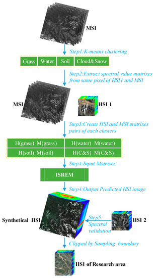
Figure 3.
Workflow of ISREM in the study area.
2.5. Mapping Coverage of NPS
2.5.1. Feature Extraction
When the HJ-1A CCD MSI was enhanced in spectral resolution by the ISREM in this paper, the band numbers were increased from 4 to 115, and the spectral resolution was enhanced to ~5 nm. However, this does not mean that adequate spectral information can achieve better recognition ability. Previous studies have shown that the classification accuracy first increases and then decreases with increasing feature dimensions in the case of limited samples, which is called the Hughes phenomenon [27,28]. To obtain better regression results for NPS, the classification features were extracted from the original wave band, first-order spectral derivative, and VIs.
The spectral difference was essential for the classification of the vegetation [29]. To map the distribution of NPS, it is necessary to find bands that can distinguish NPS from NWs. Thus, spectral differences between NPS and NWs should be determined before classifying them. In our field investigation, an SVC hr-512i ground spectrometer with a spectral range from 350 nm to 1050 nm was used to measure the spectral curves of NPS and NWs. The spectral curves of NPS and NWs were shown in Figure 4a. The spectral reflectance of the NWs was generally higher than that of NPS, which might be due to the withering period of NPS in late August. From the spectral curves, we can see intuitively that NPS and NWs could be distinguished from each other.
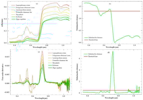
Figure 4.
Spectral characteristic curves: (a,b) are the spectral curves of the seven original grass species and the Mahalanobis distance of spectra curves between NPS and NWs. (c,d) are the first-order derivative spectral curves of the seven original grass species and the Mahalanobis distance of first-order derivative spectral curves between NPS and NWs.
In this study, the Mahalanobis distance analysis method [30] was used to select optimal bands for distinguishing NPS and NWs. The spectral reflectances of Kobresia and Stipa capillata were merged for NPS, and those of Leontopodium nanum, Potentilla chinensis Ser, Bryophyte, Polygonum sibiricum Laxm & Lamiophlomis rotate were merged for the NWs. The first-order derivative spectra were then calculated using the spectral math tool in ENVI 5.3. Then, the Mahalanobis distances of the original spectra and first-order derivative spectra between NPS and NWs were calculated.
As shown in Figure 4b,d, the average distance was chosen as the threshold of the selected band. For the original spectra, wavelengths ranging from 340 nm to 523 nm and 645 nm to 693 nm were the optimal band ranges. According to the band characteristics of the HJ-1A HSI, bands 1 to 28 and bands 65 to 75 were selected as classification features. Additionally, for first-order derivative spectra, spectral difference bands ranged from 689 nm to 755 nm. Bands 75 to 87 of the first-order derivative spectra were selected based on the band setting of the HJ-1A HSI. All selected bands of original spectra and first-order derivative spectra are shown in Table 2.
Table 2.
The features selected by Mahalanobis distance analysis from the original spectra and first-order derivative spectra. Feature bands of the fused HJ-1A/HIS were selected based on the corresponding spectral feature scale.
In addition to the selected original spectral and first derivative spectral bands, NDVI is widely used in vegetation growth monitoring, vegetation classification, and coverage modeling, and has a good ability to distinguish vegetation canopies and backgrounds [31,32]. The narrowband green normalized difference vegetation index (nGNDVI) and narrowband normalized difference vegetation index (nNDVI) are very sensitive to the greenness of vegetation [33]. Thus, the NDVI, nGNDVI and nNDVI were selected for the identification.
The biochemical and biophysical parameters within the plant leaves and the canopy, such as chlorophyll a and b, carotenoids and anthocyanin, also affected the spectral reflectance of vegetations. Biochemical indexes, such as narrowband leaf chlorophyll index (nLCI), anthocyanin reflectance index 2 (ARI2), and narrowband photochemical reflectance index (nPRI), has shown obvious differences in different grass species [34,35]. Biochemical indexes, nLCI, ARI2 and nPRI, were also selected. The final selected VIs are shown in Table 3.
Table 3.
VIs selected for regression. In the table, Rx represents the reflectance at wavelength x nm.
2.5.2. SVM and RF Regression
The SVM classifier has been widely used in land use/land cover for classification [41,42,43,44,45]. Compared with other machine learning algorithms, it has the characteristics of high precision and strong generalization ability and is suitable for remote sensing image classification of high-dimensional samples [46]. All features selected in Section 2.5.1 were combined as input images for the SVM regression in EnMAP-Box2.0 [47]. Sample image for NPS was converted from vector to raster format. The sample images must maintain the same extent and spatial resolution as the feature images. The value of the sample images was the coverage ratio of NPS. A random sample tool was used to generate the training samples and validation samples, which were in proportions of 70% and 30%, respectively. The grid search method was utilized to parameterize the SVM regression. Gaussian RBF kernel parameters (g) were initialized with a minimum value of 0.01, a maximum value of 1000, and a multiplier of 10. The regularization parameter (C) was initialized with a minimum value of 0.01, a maximum value of 1000, and a multiplier of 10. Cross-validation was used to determine the optimal parameters. The final determined parameter values were a g value of 0.1 and a C value of 100 with an epsilon (ε) insensitive loss function parameter of 12.33.
Random forest (RF) was employed as a comparison method to estimate the coverage of NPS. Previous studies have shown that RF has been widely used in remote sensing classification [48,49,50]. In recent years, RF has also performed well in grassland classification and identification [12]. For the RF regression, the number of trees was 100, and the number of features was 54. The stop criteria to stop splitting were as follows: (1) the minimum number of samples in a node is 1.0 and (2) the minimum impurity in a node is 0. Then, the selected features and training sample raster files with these parameters were used to parameterize the RF regression model, which was used to retrieve the coverage of NPS.
2.6. Evaluation Indexes of Spectral Enhancement Methods
The Pearson correlation coefficient (Pearson’s r), spectral angle mapper (SAM), erreur relative globale adimensionnelle de synthèse (ERGAS), and universal image quality index (UIQI) were adopted to assess the accuracy of the spectral enhancement methods. Pearson’s r between the same band from original HSI and synthetic HSI reflects the degree of consistency between them. The value range of the Pearson’s r was 0 to 1. The closer the value was to 1, the closer the synthesized image band was to the original band. The SAM is related to spectral distortion [51]. A lower SAM value represents better algorithm performance (the ideal value is 0). ERGAS [52] is mainly related to radiometric distortion. The closer the value is to 0, the better the algorithm performs (the ideal value is 0). UIQI [53] comprehensively considers three factors: related loss, brightness distortion and contrast distortion, and the values range from −1 to 1 (ideally 1).
3. Results
3.1. Predicted Spectra of the ISREM Compared with Those of the CRISP and SREM
3.1.1. Predicted Spectral Curve Comparison of the Three Algorithms
The spectra of the four types of ground surfaces (grassland, bare land, water and snow) were extracted from the synthetic images created by the ISREM compared with the CRISP, SREM and original images. The spectral values of each kind of ground object were randomly selected from the same position of the original image and the synthetic images generated by the CRISP, SREM and ISREM. The final spectra of each kind of ground surface were calculated by the average value and organized in the four different images shown in Figure 5. Generally, the spectral curve vibrated considerably at wavelengths of 460 nm to 520 nm and gradually smoothed out at wavelengths of 520 nm to 950 nm. In Figure 5a,c,d, the spectral curve of the ISREM was closer to the original image than those of the CRISP and SREM, especially at wavelengths of 750 nm to 950 nm. In Figure 5b, the spectral curves of the ISREM and SREM performed better than those of the CRISP.
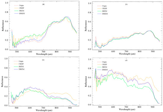
Figure 5.
Spectral comparison between the original image and synthetic image created by CRISP, SREM, and ISREM, respectively. (a) represents the spectra of grassland, (b)represents the spectra of bare land; (c) represent the spectra of water and, and (d) represents the spectra of snow.
3.1.2. Statistical Comparison of the Three Algorithms
To further compare the performance of the three algorithms, four central bands of NIR (band 107,862 nm), red (band 61, 647 nm), green (band 39, 585 nm) and blue (band 02,434 nm) bands, were extracted, and the Pearson’s r between the central bands and original bands from the ISREM, CRISP and SREM were calculated. As shown in Table 4, the Pearson’s r of the three algorithms were all above 0.9. The Pearson’s r of the ISREM were significantly higher than those of the other two methods in bands 2 (blue) and 107 (NIR) and slightly higher in bands 39 (green) and 61 (red). The average Pearson’s r indicated that the order of the performance of the three methods was ISREM > SREM > CRISP. In terms of the Pearson’s r, the ISREM performed the best in both the four selected bands and in the average value.
Table 4.
Pearson’s r between selected bands and original bands using ISREM, SREM, and CRISP.
As shown in Table 5, the ISREM performed better than the SREM and CRISP when considering SAM, ERGAS and UIQI. The value of ERGAS that were obtained from the ISREM and SREM reached a satisfactory level. The SAM value obtained from the ISREM also performed very well compared with the other two algorithms. Although the UIQI values of the three algorithms were not as high as those in the existing literature [54], the ISREM still performed the best.
Table 5.
Average cumulative quality indexes of ISREM, CRISP, and SREM.
3.2. Coverage of NPS Provided by SVM and RF Regression
The HSI produced by ISREM was used as the original data source for the SVM and RF regressions. First, we combined 39 original bands, 12 first-order bands, and 6 VIs to create an input parameter from the HSI. Then, 255 samples were randomly divided into two categories: 178 training samples and 77 verification samples. To evaluate the spectral enhancement ability of the ISREM, the original multispectral data were also used for regression. Finally, the regression results of NPS were calculated by the SVM and RF, respectively.
3.2.1. Result of SVM and RF Regression
According to the result of species coverage percentage by SVM regression, the coverage percentage of NPS was ranged from 0% to 91% and then divided into 9 grades: 0–10, 10–20, 20–30, 30–40, 40–50, 50–60, 60–70, 70–80, and >80, as shown in Figure 6a. The RF regression of NPS was also carried out. The coverage of NPS ranged from 4% to 87%. A spatial distribution coverage map of NPS with the same coverage grades of RF regression is shown in Figure 6b. Generally, the coverage grade maps of NPS estimated by SVM and RF regressions are consistent. As shown in Figure 6, the low coverage areas of NPS were mainly distributed in the gathering places of the county seat, river valleys, and mountains, while high coverage areas are mainly distributed in the pasture around the town and the sunlit slope of some mountains. This is quite consistent with the results of our field investigation.
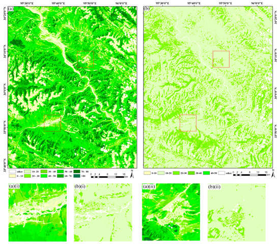
Figure 6.
Grassland coverage maps produced by two regressions using ISREM HSI. (a) is NPS abundance level map provide by SVM regression, (a)(i) and (a)(ii) are locally enlarged views of Qumalai and Zhiduo county; (b) is the NPS abundance level map provided by RF regression, (b)(i) and (b)(ii) are the locally enlarged views of Qumalai and Zhiduo county.
3.2.2. Accuracy Evaluation
To quantitatively explore the ability of the ISREM to identify grassland in the study area, the other synthetic HSIs (SREM and CRISP) and the original MSI were used as the comparative data for the regression of the coverage of NPS. For the three generated HSIs, the regression methods in Section 2.5.2 were applied to obtain the abundance information. For the original MSI, the four original bands, VIs and ARI2 in Table 3, were used as input parameters for the SVM and RF regressions.
All 77 verification samples, which were independent of the training samples, were reserved for accuracy verification. The coverage value of the sample pixels was used as a reference to estimate the values. For each validation sample, the difference between the predicted value and actual value was calculated. The quantity and proportion with the difference of less than 10% (0–10%) and less than 20% (0–20%) were used to evaluate the recognition ability of the four images to NPS. The larger number in the threshold (0–10%, 0–20%), the better image performed. As shown in Table 6, ISREM made the largest number of both 0–10% and 0–20%, which means ISREM has shown a recognition ability of NPS.
Table 6.
The statistic results of four images using SVM and RF regression (the number of all validation samples is 77. A count of 0–10% and a count of 0–20% represent the number of samples whose difference between the sample value and the estimated value is less than 10% and 20%. Proportion is the ratio of the count value (count of 0–10%, count of 0–20%) to the number of all validation samples.
3.2.3. Degradation Map of Research Area
A degradation map (Shown in Figure 7) was produced according to grassland degradation criterion in the literature [55]. Five grassland degradation levels were described as non-degradation (≥75%), mild degradation (55%~75%), moderate degradation (35%~55%), severe degradation (20~35%), and extreme degradation (≦20%) by the coverage of NPS. As shown in Table 7, moderate and severe degradation areas account for more than 60% of the study area. These areas are mainly distributed in the valley and around the town. Non and mild degradation account for only 19.63% and are mainly distributed in the high mountain slopes, which are difficult to reach. This is consistent with the coverage of NPS.
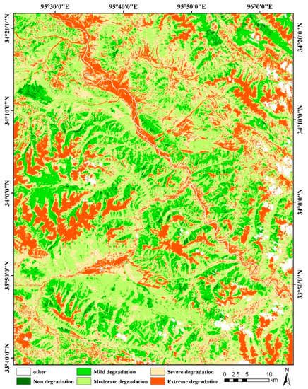
Figure 7.
Degradation map of a research area based on the coverage map of NPS generated by SVM regression using the ISREM HSI.
Table 7.
Statistics of five grassland degradation levels based on the coverage of NPS.
4. Discussion
4.1. Improvements of ISREM
The SREM was first proposed in 2014 and successfully applied in mineral alteration information extraction. Although the SREM can achieve better spectral and spatial accuracies, it relies too much on pure spectra. These pure spectra were used as spectral predictions for predicting the HSI, which were determined by the minimum spectral angle. However, mixed pixels are common in satellite HSI due to their low spatial resolution, especially in the mixed vegetation areas of the TRHR. Thus, in this study, ISREM made three improvements: (1) Clustering of the overlapping image area was carried out, and the overlapping image was clustered into several types. The average spectra were then extracted for the different types of clustered areas. (2) These average spectra were taken as “pure spectra”, and the weighted spectral angle was used for each pixel of the predicted image. (3) The ISREM can be used in nonoverlapping regions of MSI and HSI; therefore, the coverage of hyperspectral data was expanded and given a higher spatial resolution.
As shown in Section 3.1, the proposed ISREM indeed performed better than both the SREM and CRISP in the spectral and statistical comparison using the HJ-1A MSI and HSI. This might have been caused by two reasons. (1) The difficulty of obtaining pure spectra makes it difficult for the SREM to achieve a better spectral enhancement. (2) To some extent, the weighted spectral angle of “pure spectra” might improve the stability of the ISREM and reduce the effect of mixed spectra on spectral enhancement. Despite the good performance of the ISREM, it focused on mapping grassland degradation in the TRHR, and the data were restricted to HJ-1A MSI and HSI. The ISREM might have the potential for other image data and applications, and this will be explored in the future.
4.2. Potential of Spectral Enhancement in Monitoring Grassland Degradation of the TRHR
Compared to the original MSI in Section 4.2, the predicted HSI had a better performance in mapping NPS in a typical area of the TRHR. HSI can distinguish ground features with similar spectra because of their high spectral resolutions. This also proves that HSI have more potential in mapping grassland degradation in the TRHR [7].
However, limited by the design characteristics of hyperspectral remote sensing sensors, HSI usually has disadvantages, such as low spatial resolution and small spatial coverage. Previous studies have focused on the enhancement of the spectral resolution and have achieved good results [56], while there is very little effort on expanding the spatial coverage of HSI. In this study, the coverage of the HSI was improved by enhancing the spectral resolution of the MSI. Therefore, theoretically, as long as there are small overlaps between the HSI and MSI in the study area, the MSI can be simulated as HSI. This is of great significance for the research areas where remote sensing images, especially HSIs, are scarce.
Although global satellite image data are rapidly growing, relevant image data for the TRHR area, especially effective image data, are still scarce. When collecting remote sensing images to study the degradation of grassland components in a typical area of the TRHR, we found that there were few available HSIs of the study area. Taking HJ-1A imagery data as an example, the only available HSI in the study area was captured in 2013, which was six years before our latest sampling date, making it difficult to guarantee the timeliness of the data. There were two reasons for this: (1) affected by the plateau climate, the grassland growing season in the TRHR is mainly from May to September each year. This short “time window” of less than five months resulted in a significant reduction in the opportunity to obtain useful images; (2) during the growing season, there are many more convective weather and high cloud cover events in the TRHR area, leading most of the images to be unusable. The scarcity of data brings great challenges to grassland degradation research in the TRHR area.
Therefore, the ISREM proposed in this paper can expand the spatial coverage of HSI, enhance the spectral resolution of MSI, and provide a method for obtaining useful data sources. This approach also provided a technical reference for related applications for which it is difficult to directly obtain pure pixels. In addition, by comparing the synthetic HSI with the original MSI, the application potential of HSI in NWs identification was further verified.
5. Conclusions
In this paper, an improved spectral resolution enhancement method for HSI was presented, with the aim of generating a wider HSI located in a typical area of the TRHR. A clustering and weighted spectral angle method was first used as a substitute for pure pixels in generating the transformation matrix. Then, the application of the synthetic HSI to identify NPS in typical areas of the TRHR was carried out using two widely used regression algorithms (RF & SVM). Finally, the coverage maps of NPS were produced. The experiments demonstrated that the clustering and weighted spectral angle provided a better and more stable transformation matrix for predicting the HSI and that the ISREM outperformed two existing spectral resolution enhancement methods in both spectral similarity and correlation with the original reference HSI. Additionally, due to the lack of dependence on pure pixels, the ISREM has more advantages in application scenarios where it is difficult to obtain pure pixels. This alternative clustering and weight spectral angle method may make it universally applicable. The experiments on NPS recognition further proved that HSI generated by ISREM are more advantageous than MSI for identifying NPS. The original purpose of the ISREM was to solve the difficulty in obtaining time- and location-appropriate hyperspectral remote sensing images of the TRHR. Although the method has been shown to work in grassland identification, its application in other scenarios still needs to be further verified. More broadly, the generation of the transformation matrix in the ISREM could be further discussed.
Author Contributions
Conceptualization, B.W. and R.A.; methodology, B.W.; software, B.W. and T.J.; validation, F.X. and F.J.; formal analysis B.W.; investigation, B.W., T.J. and F.X.; resources, F.X.; data curation, T.J.; writing—original draft preparation, B.W.; writing—review and editing, R.A.; visualization, T.J.; supervision, F.J.; project administration, R.A.; funding acquisition, R.A. All authors have read and agreed to the published version of the manuscript.
Funding
This work is supported by the National Nature Science Foundation of China (No. 41871326; 41271361); Jiangsu Province Key R&D Plan (No. BE2017115).
Acknowledgments
We express our heartfelt gratitude for Zetian Ai, Lijun Huang, Shengyin Zhao, Meiru Zhu, Yina Hu and Xiaoling Zhou for their work of field samples collection. We would like to thank professor Yuehong Chen for his English language modification for this article. We are thankful to anonymous reviewers for their constructive and thoughtful inputs in the manuscript.
Conflicts of Interest
The authors declare no conflict of interest.
References
- Yang, S.; Feng, Q.; Liang, T.; Liu, B.; Zhang, W.; Xie, H. Modeling grassland above-ground biomass based on artificial neural network and remote sensing in the Three-River Headwaters Region. Remote Sens. Environ. 2018, 204, 448–455. [Google Scholar] [CrossRef]
- Ge, J.; Meng, B.; Liang, T.; Feng, Q.; Gao, J.; Yang, S.; Huang, X.; Xie, H. Modeling alpine grassland cover based on MODIS data and support vector machine regression in the headwater region of the Huanghe River, China. Remote Sens. Environ. 2018, 218, 162–173. [Google Scholar] [CrossRef]
- Shen, H.; Zhang, L.; Huang, B.; Li, P. A MAP approach for joint motion estimation, segmentation, and super resolution. IEEE Trans. Image Process. 2007, 16, 479–490. [Google Scholar] [CrossRef] [PubMed]
- Zhang, H.; Zhang, L.; Shen, H. A super-resolution reconstruction algorithm for hyperspectral images. Signal Process. 2012, 92, 2082–2096. [Google Scholar] [CrossRef]
- Zhang, L.; Zhang, H.; Shen, H.; Li, P. A super-resolution reconstruction algorithm for surveillance images. Signal Process. 2010, 90, 848–859. [Google Scholar] [CrossRef]
- Laben Craig, A.; Brower Bernard, V. Process for Enhancing the Spatial Resolution of Multispectral Imagery Using Pan-Sharpening. United States Patent US 6011875 A, 28 October 2015. [Google Scholar]
- Ai, Z.; An, R.; Chen, Y.; Huang, L. Comparison of hyperspectral HJ-1A/HSI and multispectral Landsat 8 and Sentinel-2A imagery for estimating alpine grassland coverage in the Three-River Headwaters region. J. Appl. Remote Sens. 2019, 13, 014504. [Google Scholar] [CrossRef]
- Chi, M.; Feng, R.; Bruzzone, L. Classification of hyperspectral remote-sensing data with primal SVM for small-sized training dataset problem. Adv. Space Res. 2008, 41, 1793–1799. [Google Scholar] [CrossRef]
- Sun, X.; Zhang, L.; Yang, H.; Wu, T.; Cen, Y.; Guo, Y. Enhancement of Spectral Resolution for Remotely Sensed Multispectral Image. IEEE J. Sel. Top. Appl. Earth Obs. Remote Sens. 2014, 8, 1–14. [Google Scholar] [CrossRef]
- Winter, M.E.; Winter, E.M.; Beaven, S.G.; Ratkowski, A.J. Hyperspectral image sharpening using multispectral data. Def. Secur. 2005, 5806, 794–803. [Google Scholar] [CrossRef]
- Liu, J.; Xu, X.; Shao, Q. Grassland degradation in the “Three-River Headwaters” region, Qinghai Province. J. Geogr. Sci. 2008, 18, 259–273. [Google Scholar] [CrossRef]
- Fan, J.-W.; Shao, Q.-Q.; Liu, J.-Y.; Wang, J.-B.; Harris, W.; Chen, Z.-Q.; Zhong, H.-P.; Xu, X.-L.; Liu, R.-G. Assessment of effects of climate change and grazing activity on grassland yield in the Three Rivers Headwaters Region of Qinghai–Tibet Plateau, China. Environ. Monit. Assess. 2009, 170, 571–584. [Google Scholar] [CrossRef] [PubMed]
- Wang, X.; Dong, S.; Yang, B.; Li, Y.; Su, X. The effects of grassland degradation on plant diversity, primary productivity, and soil fertility in the alpine region of Asia’s headwaters. Environ. Monit. Assess. 2014, 186, 6903–6917. [Google Scholar] [CrossRef] [PubMed]
- Shen, X.-J.; An, R.; Feng, L.; Ye, N.; Zhu, L.; Li, M. Vegetation changes in the Three-River Headwaters Region of the Tibetan Plateau of China. Ecol. Indic. 2018, 93, 804–812. [Google Scholar] [CrossRef]
- Tong, Q.; Xue, Y.; Zhang, L. Progress in Hyperspectral Remote Sensing Science and Technology in China Over the Past Three Decades. IEEE J. Sel. Top. Appl. Earth Obs. Remote Sens. 2013, 7, 70–91. [Google Scholar] [CrossRef]
- Liang, T.; Yang, S.; Feng, Q.; Liu, B.; Zhang, R.; Huang, X.; Xie, H. Multi-factor modeling of above-ground biomass in alpine grassland: A case study in the Three-River Headwaters Region, China. Remote Sens. Environ. 2016, 186, 164–172. [Google Scholar] [CrossRef]
- Ru, A.; Caihong, L.; Huilin, W.; Daping, J.; Mengqiu, S.; Ballard, J.A.Q. Remote sensing identification of rangeland degradation using Hyperion HSI in a typical area for Three-River Headwater Region. Geomat. Inf. Sci. Wuhan Univ. 2018, 3, 399–405. (In Chinese) [Google Scholar] [CrossRef]
- Xu, S.; Shang, Z. The Three-stage Species Niche and Reproductive Characteristics of Poisonous Weeds in the three-stages of the Secondary Vegetation’s Formation of ‘bare land’ degraded grassland in the Three Rivers Source region, Qinghai-Tibetan plateau. Acta Agrestia Sin. 2019, 27, 949–955. (In Chinese) [Google Scholar] [CrossRef]
- Ai, Z.; An, R.; Lu, C.; Chen, Y. Mapping of native plant species and noxious weeds to investigate grassland degradation in the Three-River Headwaters region using HJ-1A/HSI imagery. Int. J. Remote Sens. 2019, 41, 1813–1838. [Google Scholar] [CrossRef]
- Niu, L.M.; Meng, J.H.; Wu, B.F.; Chen, X.Y.; DU, X.; Zhang, F.F. Research on standard preprocessing flow for HJ-1A HSI level 2 data product. Remote Sens. Land Resour. 2011, 1, 77–82. (In Chinese) [Google Scholar]
- Teillet, P.; Guindon, B.; Goodenough, D. On the Slope-Aspect Correction of Multispectral Scanner Data. Can. J. Remote Sens. 1982, 8, 84–106. [Google Scholar] [CrossRef]
- Yokoya, N.; Grohnfeldt, C.; Chanussot, J. Hyperspectral and Multispectral Data Fusion: A comparative review of the recent literature. IEEE Geosci. Remote Sens. Mag. 2017, 5, 29–56. [Google Scholar] [CrossRef]
- Adam, E.; Mutanga, O.; Rugege, D. Multispectral and hyperspectral remote sensing for identification and mapping of wetland vegetation: A review. Wetl. Ecol. Manag. 2009, 18, 281–296. [Google Scholar] [CrossRef]
- Loncan, L.; Almeida, L.B.; Bioucas-Dias, J.M.; Briottet, X.; Chanussot, J.; Dobigeon, N.; Fabre, S.; Liao, W.; Licciardi, G.A.; Simoes, M.; et al. Hyperspectral Pansharpening: A Review. IEEE Geosci. Remote Sens. Mag. 2015, 3, 27–46. [Google Scholar] [CrossRef]
- Heylen, R.; Parente, M.; Gader, P. A Review of Nonlinear Hyperspectral Unmixing Methods. IEEE J. Sel. Top. Appl. Earth Obs. Remote Sens. 2014, 7, 1844–1868. [Google Scholar] [CrossRef]
- Zhuang, L.; Zhang, B.; Gao, L.; Li, J.; Plaza, J. Normal Endmember Spectral Unmixing Method for Hyperspectral Imagery. IEEE J. Sel. Top. Appl. Earth Obs. Remote Sens. 2014, 8, 2598–2606. [Google Scholar] [CrossRef]
- Hughes, G. On the mean accuracy of statistical pattern recognizers. IEEE Trans. Inf. Theory 1968, 14, 55–63. [Google Scholar] [CrossRef]
- Du, P.J.; Xia, J.S.; Xue, Z.H.; Tan, K.; Su, H.J.; Bao, R. Review of hyperspectral remote sensing image classification. J. Remote Sens. 2016, 2, 236–256. (In Chinese) [Google Scholar] [CrossRef]
- McGwire, K. Hyperspectral Mixture Modeling for Quantifying Sparse Vegetation Cover in Arid Environments. Remote Sens. Environ. 2000, 72, 360–374. [Google Scholar] [CrossRef]
- Lin, H.-J.; Zhang, H.-F.; Gao, Y.-Q.; Li, X.; Yang, F.; Zhou, Y.-F. Mahalanobis distance based hyperspectral characteristic discrimination of leaves of different desert tree species. Guang Pu Xue Yu Guang Pu Fen Xi = Guang Pu 2014, 34, 3358–3362. [Google Scholar]
- Lu, Q.; Zhao, N.; Wu, S.; Dai, E.; Gao, J. Using the NDVI to analyze trends and stability of grassland vegetation cover in Inner Mongolia. Theor. Appl. Clim. 2018, 135, 1629–1640. [Google Scholar] [CrossRef]
- Payero, J.O.; Neale, C.M.U.; Wright, J.L. Comparison of eleven vegetation indices for estimating plant height of alfalfa and grass. Appl. Eng. Agric. 2004, 20, 385–393. [Google Scholar] [CrossRef]
- Mutanga, O.; Skidmore, A.K. Narrow band vegetation indices overcome the saturation problem in biomass estimation. Int. J. Remote Sens. 2004, 25, 3999–4014. [Google Scholar] [CrossRef]
- Asner, G.P.; Jones, M.O.; Martin, R.E.; Knapp, D.; Hughes, R.F. Remote sensing of native and invasive species in Hawaiian forests. Remote Sens. Environ. 2008, 112, 1912–1926. [Google Scholar] [CrossRef]
- Rosso, P.H.; Ustin, S.L.; Hastings, A. Mapping marshland vegetation of San Francisco Bay, California, using hyperspectral data. Int. J. Remote Sens. 2005, 26, 5169–5191. [Google Scholar] [CrossRef]
- Tucker, C.J. Red and photographic infrared linear combinations for monitoring vegetation. Remote Sens. Environ. 1979, 8, 127–150. [Google Scholar] [CrossRef]
- Gitelson, A.A.; Kaufman, Y.J.; Merzlyak, M.N. Use of a green channel in remote sensing of global vegetation from EOS-MODIS. Remote Sens. Environ. 1996, 58, 289–298. [Google Scholar] [CrossRef]
- Botha, E.; LeBlon, B.; Zebarth, B.; Watmough, J. Non-destructive estimation of potato leaf chlorophyll from canopy hyperspectral reflectance using the inverted PROSAIL model. Int. J. Appl. Earth Obs. Geoinf. 2007, 9, 360–374. [Google Scholar] [CrossRef]
- Datt, B. A New Reflectance Index for Remote Sensing of Chlorophyll Content in Higher Plants: Tests using Eucalyptus Leaves. J. Plant Physiol. 1999, 154, 30–36. [Google Scholar] [CrossRef]
- Gamon, J.A.; Serrano, L.; Surfus, J.S. The photochemical reflectance index: An optical indicator of photosynthetic radiation use efficiency across species, functional types, and nutrient levels. Oecologia 1997, 112, 492–501. [Google Scholar] [CrossRef]
- Mountrakis, G.; Im, J.; Ogole, C. Support vector machines in remote sensing: A review. ISPRS J. Photogramm. Remote Sens. 2011, 66, 247–259. [Google Scholar] [CrossRef]
- Antonarakis, A.S.; Richards, K.; Brasington, J. Object-based land cover classification using airborne LiDAR. Remote Sens. Environ. 2008, 112, 2988–2998. [Google Scholar] [CrossRef]
- Pandey, P.C.; Koutsias, N.; Petropoulos, G.P.; Srivastava, P.K.; Ben Dor, E. Land use/land cover in view of earth observation: Data sources, input dimensions, and classifiers—A review of the state of the art. Geocarto Int. 2019, 1–32. [Google Scholar] [CrossRef]
- Fauvel, M.; Benediktsson, J.A.; Chanussot, J.; Sveinsson, J.R. Spectral and Spatial Classification of Hyperspectral Data Using SVMs and Morphological Profiles. IEEE Trans. Geosci. Remote Sens. 2008, 46, 3804–3814. [Google Scholar] [CrossRef]
- Dixon, B.; Candade, N. Multispectral landuse classification using neural networks and support vector machines: One or the other, or both? Int. J. Remote Sens. 2007, 29, 1185–1206. [Google Scholar] [CrossRef]
- Du, P.; Tan, K.; Xing, X. A novel binary tree support vector machine for hyperspectral remote sensing image classification. Opt. Commun. 2012, 285, 3054–3060. [Google Scholar] [CrossRef]
- Van Der Linden, S.; Rabe, A.; Held, M.; Jakimow, B.; Leitão, P.J.; Okujeni, A.; Schwieder, M.; Suess, S.; Hostert, P. The EnMAP-Box—A Toolbox and Application Programming Interface for EnMAP Data Processing. Remote Sens. 2015, 7, 11249–11266. [Google Scholar] [CrossRef]
- Peerbhay, K.; Mutanga, O.; Lottering, R.; Ismail, R. Mapping Solanum mauritianum plant invasions using WorldView-2 imagery and unsupervised random forests. Remote Sens. Environ. 2016, 182, 39–48. [Google Scholar] [CrossRef]
- Belgiu, M.; Drăguț, L. Random forest in remote sensing: A review of applications and future directions. ISPRS J. Photogramm. Remote Sens. 2016, 114, 24–31. [Google Scholar] [CrossRef]
- Feng, Q.; Liu, J.; Gong, J. UAV Remote Sensing for Urban Vegetation Mapping Using Random Forest and Texture Analysis. Remote Sens. 2015, 7, 1074–1094. [Google Scholar] [CrossRef]
- Kruse, F.; Lefkoff, A.; Boardman, J.; Heidebrecht, K.; Shapiro, A.; Barloon, P.; Goetz, A. The spectral image processing system (SIPS)—Interactive visualization and analysis of imaging spectrometer data. Remote Sens. Environ. 1993, 44, 145–163. [Google Scholar] [CrossRef]
- Ranchin, T.; Wald, L. Fusion of high spatial and spectral resolution images: The ARSIS concept and its implementation. Photogramm. Eng. Remote Sens. 2000, 66, 49–61. [Google Scholar]
- Wang, Z.; Bovik, A.C. A universal image quality index. IEEE Signal Process. Lett. 2002, 9, 81–84. [Google Scholar] [CrossRef]
- Wang, G.; Zhang, L.; Sun, X.; Yang, H.; Jiang, H.; Tong, Q. Mineral alteration information extraction based on SREM fusion data. Editor. Comm. Earth Sci. J. China Univ. Geosci. 2015, 8, 1330–1338. (In Chinese) [Google Scholar] [CrossRef]
- Pan, D. Study on the Types and Grade Partition Criterion of “Black Soil Type” Degraded Grassland in the “Three-River Headwater” Region. Master’s Thesis, Gansu Agricultural University, Lanzhou, China, 2007. (In Chinese). [Google Scholar]
- Meng, X.; Shen, H.; Li, H.; Zhang, L.; Fu, R. Review of the pansharpening methods for remote sensing images based on the idea of meta-analysis: Practical discussion and challenges. Inf. Fusion 2019, 46, 102–113. [Google Scholar] [CrossRef]


© 2020 by the authors. Licensee MDPI, Basel, Switzerland. This article is an open access article distributed under the terms and conditions of the Creative Commons Attribution (CC BY) license (http://creativecommons.org/licenses/by/4.0/).