QCam: sUAS-Based Doppler Radar for Measuring River Discharge

Abstract

The U.S. Geological Survey is actively investigating remote sensing of surface velocity and river discharge (discharge) from satellite-, high altitude-, small, unmanned aircraft systems- (sUAS or drone), and permanent (fixed) deployments. This initiative is important in ungaged basins and river reaches that lack the infrastructure to deploy conventional streamgaging equipment. By coupling alternative discharge algorithms with sensors capable of measuring surface velocity, streamgage networks can be established in regions where data collection was previously impractical or impossible. To differentiate from satellite or high-altitude platforms, near-field remote sensing is conducted from sUAS or fixed platforms. QCam is a Doppler (velocity) radar mounted and integrated on a 3DR^© Solo sUAS. It measures the along-track surface velocity by spot dwelling in a river cross section at a vertical where the maximum surface velocity is recorded. The surface velocity is translated to a mean-channel (mean) velocity using the probability concept (PC), and discharge is computed using the PC-derived mean velocity and cross-sectional area. Factors including surface-scatterer quality, flight altitude, propwash, wind drift, and sample duration may affect the radar-returns and the subsequent computation of mean velocity and river discharge. To evaluate the extensibility of the method, five science flights were conducted on four rivers of varying size and dynamics and included the Arkansas River, Colorado (CO), USA (two events); Salcha River near Salchaket, Alaska (AK), USA; South Platte River, CO, USA; and the Tanana River, AK, USA. QCam surface velocities and river discharges were compared to conventional streamgaging methods, which represented truth. QCam surface velocities for the Arkansas River, Salcha River, South Platte River, and Tanana River were 1.02 meters per second (m/s) and 1.43 m/s; 1.58 m/s; 0.90 m/s; and 2.17 m/s, respectively. QCam discharges (and percent differences) were 9.48 (0.3%) and 20.3 cubic meters per second (m³/s) (2.5%); 62.1 m³/s (−10.4%); 3.42 m³/s (7.3%), and 1579 m³/s (−18.8%). QCam results compare favorably with conventional streamgaging and are a viable near-field remote sensing technology that can be operationalized to deliver real-time surface velocity, mean velocity, and river discharge, if cross-sectional area is available.

1. Introduction

River discharge (discharge or streamflow) is an important component of the water cycle, and an accurate accounting can be accomplished by monitoring the spatial and temporal variations in discharge. These variations inform decision makers on water-resource related issues, given two-fifths of the global rainfall that occurs over land is routed by rivers to the ocean [1].

In 1888, the U.S. Geological Survey (USGS) constructed a camp and the first USGS streamgage on the Rio Grande near Embudo, New Mexico [2]. The objective was to establish a training center for the first hydrographers of the Irrigation Survey, a Bureau added to the USGS under the direction of John Wesley Powell [2]. In 2020, the USGS operates 10,330 streamgages, which constitutes one of the largest streamgage networks in the world [3]. Approximately 80,000 discharge measurements are made annually to create or maintain rating curves that relate a stage (water level) to a discharge (stage-discharge rating). These data are used by various end users for water resources planning, forecasting, and early warning networks for floods and droughts [3].

River discharge is measured at a cross section or at a reach and computed using various metrics including hydraulic grade (slope), cross-sectional area, top width, depth, mean-channel (mean) velocity, and a friction factor [4,5,6]. Since the inception of the Embudo streamgage, methods and instruments have evolved from mechanical current meters [4,5,6] to hydroacoustics. Acoustic Doppler current profilers (ADCPs) and acoustic Doppler velocimeters (ADVs) revolutionized the practice of streamgaging and are used operationally today by hydrographers [7,8,9,10,11,12,13,14]. Mechanical current meters, hydroacoustics, and their associated computational methods are effective tools for measuring discharge; however, practitioners are constrained largely to placing instruments in the water column. Where infrastructure (bridges or boat access) is lacking or extreme river discharges limit access by boat or by wading, conventional methods can result in data gaps.

Remote-sensing platforms offer an alternative to in-river measurements when safety and accessibility are in question. Beginning in the late 20th and early 21st centuries, discharge could be measured using remote-sensing platforms, and the workflow to deliver discharge time-series in rivers was a reality. Hydrologic remote sensing focused on high-altitude or satellite-based products. Traditional ground-based and hydraulically-modeled discharges have been coupled with various satellite platforms to compute discharge using remote sensing and include (1) radar altimetry from National Aeronautics and Space Administration (NASA) satellites TOPEX/Poseidon, ERS-1, 2; ENVISAT; NASA SRTM; NASA Jason-2; SARAL; CryoSat-2; and Sentinel 3A [15,16,17,18,19,20,21,22,23,24,25,26,27]; (2) NASA Landsat imagery [28,29,30,31,32,33,34,35,36]; (3) AMSR-E [37], and (4) NASA SWOT [1,38,39,40,41,42]. For example, satellite-based discharges were derived for the Yukon River at Eagle and Stevens Point, Alaska, based on water-surface area, slope, and water-surface height [25]. When combined with four USGS discharge measurements of varying magnitude, the satellite-based discharges were within 10 percent (%) of actual discharges during a five-year period [25].

To differentiate from satellite or high-altitude platforms, near-field remote sensing is conducted from platforms such as small, unmanned aircraft systems (sUAS), bridges, and cable stays. In 1996, the USGS initiated Hydro 21, which represented an effort to trial near-field remote sensing methods to measure surface velocity, mean-channel (mean) velocity, river depth, and compute discharge from helicopters and permanent deployments [43,44,45,46,47,48]. Particle image velocimetry (PIV) and particle tracking velocimetry (PTV) emerged as methods for measuring surface velocity and computing discharge from the ground [49,50,51,52], from small aircraft [53], and from sUAS [54,55,56]. Portable [57,58] and permanent Doppler (velocity) and pulsed (stage) radars [59,60] have been deployed to operationalize the process by delivering real-time, continuous time series of velocity and discharge.

Previous research [60] demonstrated the utility of fixed-mount radars to measure surface velocities and the probability concept (PC) algorithm to compute mean velocities. This previously published research compared (1) time series of radar- and conventional stage-discharge ratings and (2) instantaneous radar discharges to hydroacoustics, at 10 USGS streamgages where fixed-mount radars were collocated at bridges (near-field environments). A variety of hydrologic and hydraulic settings (flashy-urban basins, high-gradient mountain streams, mixed use, and large rivers), drainage areas (381 to 66,200 square kilometers [km²]), top widths (7.0 to 380 meters [m]), surface velocities (0.3 to 3.84 meters per second [m/s]), and discharges (0.12 to 4950 cubic meters per second [m³/s]) were evaluated. The radar gages were deployed for a sufficient period of time (<1 to 19 months) so that streamflow extremes could be recorded and analyzed. Streamflow exceedances were computed and ranged from approximately 0% to 5.4% and were deemed representative of the streamflow magnitudes and temporal variations, which were monitored at the collocated USGS streamgages. The results indicated that velocity and stage-radar gages can produce continuous time series of mean velocity, stage, and discharges that (1) compare favorably to stage-discharge ratings and (2) can be computed in the absence of historical data [60]. This same workflow was adopted for sUAS, which is the basis for this research.

Given the limitations of site access and costs to develop and maintain conventional stage-discharge ratings, alternative methods are needed to expand streamgage networks, particularly in ungaged basins. Satellite platforms fill a substantial void in global hydrologic studies in regions lacking streamgages because of their large-spatial scale; however, the spatial resolution can be compromised. Near-surface remote sensing platforms including sUAS-based velocity radars may offer a solution for measuring river discharge for (1) top widths ranging from 5 to 300 m; (2) remote basins such as those in Alaska, where access and infrastructure limit the utility of conventional streamgage operations; (3) extreme flow events, which may pose a safety hazard to hydrographers; and (4) satellite-based discharges (NASA SWOT) that would benefit from ground-based calibration/validation (Cal/Val).

2. Materials and Methods

This research summarizes the specifications of QCam (an sUAS-based Doppler velocity radar) and the workflow for (1) integrating a velocity radar on an sUAS, (2) developing a flight envelope, (3) conducting science flights at collocated USGS streamgages, and (4) establishing field and computational methods to compute real-time discharge from an sUAS.

2.1. QCam Specifications

QCam is a velocity radar, which is integrated on an sUAS (Figure 1). It is a relatively inexpensive sensor ($6K U.S. dollars), and its form factor is compatible with sUAS integration. QCam was developed by the USGS and Sommer Messtechnik and is a miniaturized coherent, continuous-wave (CCW) Doppler radar that operates at 24 gigahertz (GHz). QCam measures surface velocities in rivers based on the Doppler Shift exhibited by small-scale surface waves (surface scatterers) on the water surface. It is capable of measuring surface velocities in small and large rivers (5 to 300 m wide).

When QCam measurements are coupled with channel cross-sectional area, which is derived from ADCPs, stage-area ratings, lidar [56], or ground-penetrating radar (GPR) [61]; near-field remote sensing of river discharge can be computed. The platform is particularly helpful in rivers that are not accessible by wading, bridge (fixed mount), or boat or too wide to accommodate PIV or PTV flights.

QCam generates a radar spectrum in real time, which includes a measure of the surface velocity and measurement quality. The velocity radar is similar to those radars evaluated by Hydro 21 with some modifications and is calibrated by the manufacturer prior to delivery. The computed velocity is derived onboard using a digital signal processor and spectral analysis. The area occupied by the radar footprint is a function of the incidence angle and air gap. Data are transmitted remotely to a laptop computer using a LM Technology^® BlueTooth Universal Serial Bus (USB) adapter. The velocities recorded by QCam were validated in a carriage tow tank in 2015 to assess radar performance and uncertainties under controlled conditions by the Federal Institute of Metrology METAS [62] and the USGS Hydrologic Instrumentation Facility, respectively. Operating specifications for the radar are described in

Table 1. QCam and 3DR^© Solo specifications (Courtesy Sommer Messtechnik) [m, meters; mm, millimeters; s, seconds; m/s, meters per second; mm/s, millimeters per second; °, degrees; GHz, gigahertz; gm, grams].

Velocity Measurement	Comment
Detectable measurement range	0.10 to 15 m/s
Accuracy	±0.01 m/s; ±1%
Resolution	1 mm/s
Direction recognition	+/–
Measurement duration	5 to 240 s
Measurement frequency	24 GHz (K-Band)
Radar opening angle	12°
Distance to water surface	minimum 0.50 m
Necessary minimum ripple height	3 mm
Vertical inclination	measured internally
Automatic Vertical Angle Compensation	Comment
Accuracy	± 1°
Resolution	± 0.1°
3DR© Solo	Comment
Solo 3DR™ with battery	957.84 gm
Battery	495 gm
Center of lift imaginary weight	1 gm
Leg extensions, propellers, and vibrational dampeners	30 gm
QCam and 3D mount	545.12 gm
Total	2028.96 gm

.

2.2. QCam Integration

QCam was integrated on a 3DR^© Solo—a light-lift quadcopter—using a mount, which was fabricated from a MakerBot™ 3D printer. The aircraft weight and balance are extremely important to (1) maintain stability during vertical takeoff and landing (VTOL) and (2) minimize vibrational biases during data collection. The sensor and mounting system were constrained because of the weight of the radar and the distance between the bottom of the aircraft fuselage and the bottom of the aircraft legs. In addition, the mount needed to withstand hard landings, incidental flips, and potential crashes. Flight stability was optimized by upgrading the onboard GPS (Neo-M8 u-blox) and propellers (4, 10 inch MASTER AIRSCREW).

QCam operates by spot dwelling (hovering for a prescribed duration) at a specific location in a river cross section and requires a stable altitude and heading. Because of the nature of aircraft operations, vibrations (mechanical, electrical, or aerodynamic/elastic) can occur and may inhibit the ability to effectively collect velocity data. Vibration dampening of the sensor must be resistant to high, low, and resonating frequencies and was incorporated in the design. A gimballing system was considered; however, because of the weight and size requirements, it was dismissed. The radar weight distribution (center of gravity (CG) and mass moment of inertia) contributes to the aircraft stability and is dynamically important in the integration of the radar payload with the aircraft. Reducing the CG location relative to the center of lift (CL) was beneficial and aided in the stability of the aircraft during flight. By isolating the mounting system, the aircraft and sensor were not subject to vibrations, and the overall stability was improved.

2.3. QCam Flight Envelope

A flight envelope was developed for QCam to establish the environmental conditions and aircraft performance metrics, under which the aircraft can operate. Variables such as motor pod temperature, wind speed, density altitude (DA), and flight time were computed and field tested prior to receiving Department of Interior (DOI) Office of Aviation Services (OAS) approval.

2.4. Science Flights at Collocated USGS Streamgages

To evaluate the extensibility of the methods, five science flights were conducted on four rivers of varying size and dynamics and included the Arkansas River, Colorado (CO), USA (two flights); Salcha River, Alaska (AK), USA; South Platte River, CO, USA; and the Tanana River, AK, USA. Drainage areas ranged from 5252 to 66,200 km². Two test flights were conducted prior to the first science flight, where no data were collected and was convened on the Denver Federal Center, CO, USA and the South Platte River. Each of the five science flights were collocated at operational USGS streamgages. Conventional streamgaging methods served as truth and were used to measure the efficacy of the near-field remote sensing methods. The data described in this manuscript are referenced as a USGS data release [63] and included in the Supplementary Materials. USGS streamgage descriptions are referenced in the National Water Information System database [64], which is searchable by the streamgage identification number in

Table 2. Location of study areas where QCam science flights were conducted [latitude and longitude are referenced as North American Datum of 1983 (2011); USGS, U.S Geological Survey; km², square kilometers].

USGS Streamgage Identification Number	Date Collected	USGS Streamgage	Latitude	Longitude	Drainage Area (km2)
07094500	20 March 2018	Arkansas River at Parkdale, Colorado	38.4872265	−105.3736086	6369
07094500	28 June 2018	Arkansas River at Parkdale, Colorado	38.4872265	−105.3736086	6369
15484000	10 July 2018	Salcha River near Salchaket, Alaska	64.471528	−146.928056	5698
06701900	24 October 2017	South Platte River below Brush Creek near Trumbull, Colorado	39.2599913	−105.2219365	5252
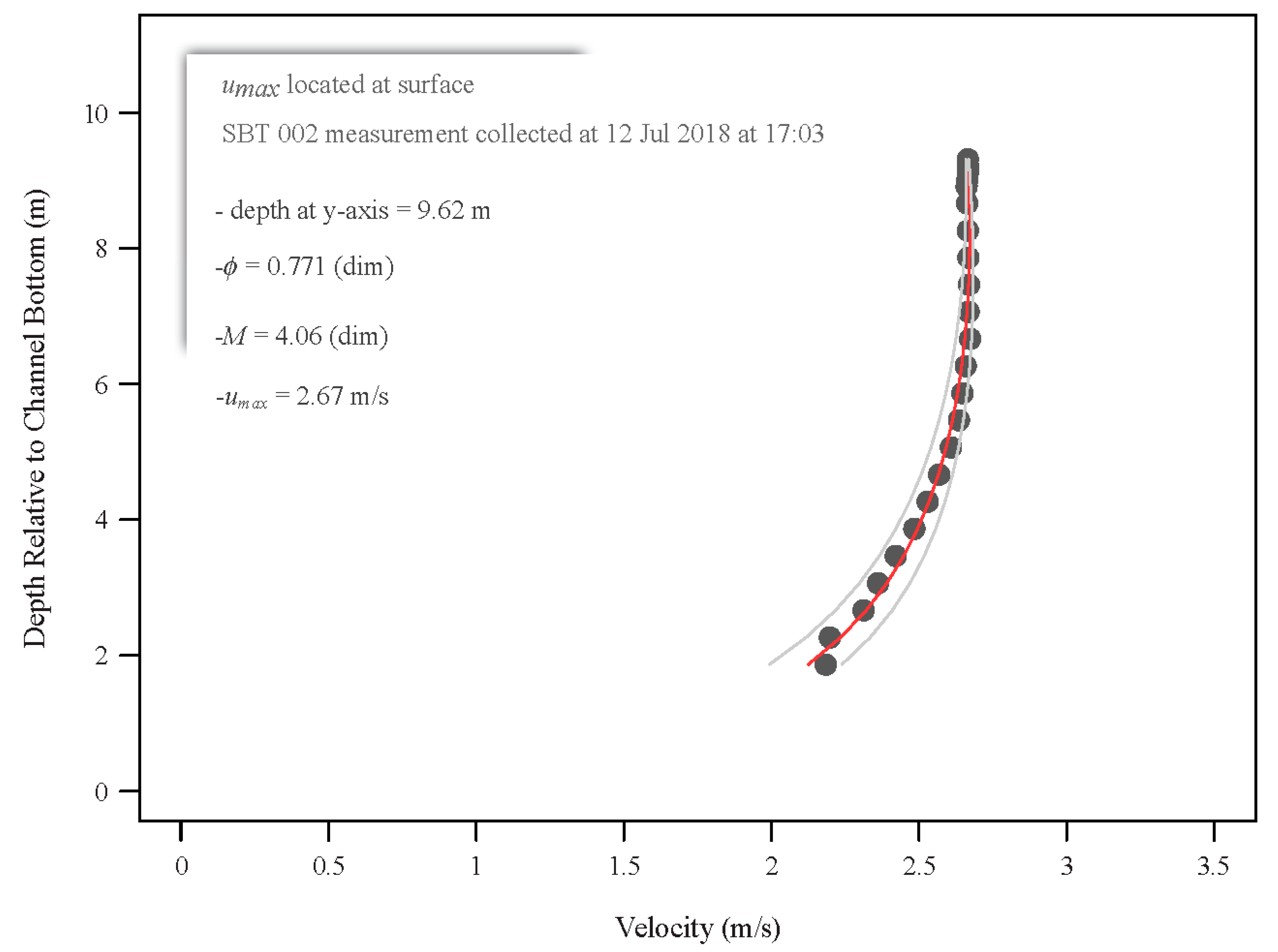
15515500	12 July 2018	Tanana River near Nenana, Alaska	64.5649444	−149.0940000	66,200

.

2.5. Field and Computational Methods

2.5.1. Conventional Streamgaging

Conventional streamgaging methods [4,5,6,7,8,9,10,11,12,13,14] are widely accepted industry standards and include stage-discharge ratings, mechanical current meters, and hydroacoustics including ADCPs and ADVs. These instruments were used to (1) collect velocity and discharge data to serve as truth, (2) measure channel bathymetry to establish a stage-area rating, (3) determine the location of the y-axis (the vertical containing the maximum (instream) velocity), and (4) measure the vertical–velocity distribution at the y-axis to compute the PC parameters ϕ (ratio between mean velocity and maximum velocity) and h/D (vertical distance from the water surface to the ratio between maximum velocity and maximum depth at the y-axis) needed to compute the mean velocity and discharge.

The maximum surface velocity is used to inform a user of the location of the y-axis and subsequently the location of the maximum velocity [60]. When rivers were wadable, the y-axis was established using surface velocity data derived from a handheld Stalker Pro II surface velocity radar (SVR) and confirmed using a SonTek FlowTracker2^® (FT2) ADV. The SVR is a 34.7 GHz velocity radar and relies on the Doppler-frequency shift to return a surface velocity. To corroborate the location of the y-axis and to validate QCam velocities, velocity data were collected to the left and right of the y-axis. Once established, the FT2 ADV was used to collect a near-surface velocity and point velocities as a function of water depth. Data were collected near the channel bottom, throughout the water column, to the water surface while minimizing air entrainment near the air-water interface [59,60]. This procedure was repeated to river left (LEW, to the left facing downstream) and river right (REW, to the right facing downstream) of the y-axis to confirm its location. When rivers were not wadable, velocity data were collected at the y-axis using a stationary bed test (SBT) from a boat. As with the FT2 ADV, SBTs were conducted to the river left and river right of the y-axis and processed in WinRiver II to characterize the velocity distribution [59,60]. Discharge was computed using QRev [12].

2.5.2. QCam Deployment

QCam was deployed to the y-axis from a prescribed take-off/return-to-launch (TO/RTL) point located near the LEW or REW. To ensure proper positioning, the distance from the TO/RTL and sUAS height was monitored using a range finder, by wading, by boat, or by launching a second sUAS, which was flown overhead and used for situational awareness. When deploying QCam, the principles used to site conventional streamgages [4] were adopted and considered only those cross sections that (1) consist of straight channels with parallel streamlines; (2) include streambeds free of large rocks, weeds, and obstructions that would create turbulence or slack water; (3) comprise cross sections that are parabolic, trapezoidal, or rectangular; (4) avoid variable flow conditions downstream from piers or channel obstructions; (5) avoid highly turbulent conditions, (6) target sections where stream velocities exceed 0.15 m/s and depths greater than 0.15 m; (7) avoid tributaries or contributing drainage; and (8) avoid wind-dominated reaches, eddies, secondary currents, and macroturbulence [4,5,6].

Spot dwell durations ranged from approximately 30 seconds (s) to 2 minutes (min) and depended on the surface-scatterer size and quality, which is a function of the radar transmission frequency and environmental factors. Velocity and radar quality data were processed onboard and transmitted wirelessly from QCam to a laptop located near the TO/RTL. The maximum transmission distance was verified during flights conducted at the Tanana River and was limited to approximately 140 m.

2.5.3. Velocity and Discharge Algorithms

Mean velocity and discharge was computed using two methods: (1) conventional methods (stage-discharge ratings; current meters/ADVs/mid-section method; and ADCPs), which are widely accepted as industry standards [4,5,6,11,12,13,14] and served to validate the QCam results, and (2) PC, a discharge algorithm based on the Chiu velocity distribution equation [65], which translates a surface velocity to a mean velocity. The PC offers two advantages when compared to conventional methods by (1) providing a mathematical basis for translating a single, surface velocity to a mean velocity and (2) resolving non-standard vertical-velocity distributions (logarithmic or power law), where the maximum velocity occurs below the water surface. It is important to note that the location of the y-axis and ϕ appear to be resilient to stage, velocity, and discharge extremes [60]. Once established for a cross section, ϕ can be used to compute a mean velocity for various streamflow conditions at a cross section a priori. When coupled with the surface velocity and cross-sectional area, discharge can be computed in real time. A comprehensive workflow is summarized below.

Surface velocities recorded by QCam were analyzed using the PC, which relies on an alternative velocity distribution equation pioneered by C.-L. Chiu [65,66,67,68,69,70,71,72,73] and is based on Shannon’s Information Entropy [74]. Velocity and depth data are collected at the y-axis, which contains the most information content (velocity = 0 and velocity = maximum velocity). The PC translates a velocity collected at the y-axis into a mean velocity and computes discharge using ϕ and a cross-sectional area.

The surface velocity measured by QCam was translated to a mean velocity using Equations (1) through (5), which offer a summary of the Chiu velocity distribution equation [65]. The velocity distribution along the y-axis in probability space is represented by Equation (1):

$$u=\frac{u_{max}}{M}ln\left[1+\left(e^M-1\right)F\left(u\right)\right]$$

(1)

where u = velocity as a function of depth at the y-axis; u_max = maximum velocity at the y-axis; M = parameter of the probability distribution used to describe the velocity distribution, $F\left(u\right)=\underset{0}{\overset{u}{\int }}f\left(u\right)du$represents the cumulative distribution function, or the probability of a randomly sampled point velocity less than or equal to u. At those cross sections where u_max occurs below the water surface, the velocity distribution at the y-axis can be characterized by Equation (2):

$$u=\frac{u_{max}}{M}ln\left[1+\left(e^M-1\right)\frac{y}{D-h}exp\left(1-\frac{y}{D-h}\right)\right]$$

(2)

where D = total distance from the channel bottom to the water surface at the y-axis, y = incremental distance from the channel bottom to water surface, h = vertical distance from the water surface to u_max. A curvilinear coordinate system [65] is used to translate the velocity distribution from probability space to physical space and is used to describe the variables h, D, and y. In those instances when u_max occurs at the water surface, the velocity distribution at the y-axis can be characterized by Equation (3):

$$u=\frac{u_{max}}{M}ln\left[1+\left(e^M-1\right)\frac{y}{D}exp\left(1-\frac{y}{D}\right)\right]$$

(3)

The probability distribution f(u) is resilient, invariant with time and water level at a channel section and, hence, M and h/D are constant at a channel cross section [68,75,76]. In practice, Equation (2) is used only when there is a clear and observed velocity distribution where u_max occurs below the water surface. In those instances, the QCam velocity is used to estimate u_max and assumes u = uD as described by Equation (4) [70]:

$$u_{max}=uDxMx\{ln\left[1+\left(e^M-1\right)\frac{1}{1-\frac{h}{D}}exp\left(1-\frac{1}{1-\frac{h}{D}}\right)\right]{\}}^{-}{}^1$$

(4)

where uD = surface velocity or u at y = D, h/D = location of u_max below the water surface at the y-axis divided by D at the y-axis. In Equation (5) the parameter ϕ, which is a function of M, can be computed using two methods. The first method relies on velocity and depth pairs obtained from the y-axis during the siting phase. Values for u_max, M(ϕ), and h/D are computed using a nonlinear estimator in R v3.4.3 [77]. By default, Equations (2) and (3) are solved using a Gauss-Newton nonlinear least squares method. The second method, which is preferred [52,67,74], relies on historical pairs of mean and maximum velocities obtained during site visits:

$$\varphi =\frac{u_{mean}}{u_{max}}=\frac{e^M}{\left(e^M-1\right)}-\frac{1}{M}$$

(5)

where ϕ = u_mean/u_max = function of M; u_mean = mean velocity. The QCam discharge is based on u_max, which is measured in real time [60] and Equation (6):

$$Q=\varphi \times u_{max}\times A$$

(6)

where Q = discharge and A = cross-sectional area.

3. Results

3.1. QCam Integration

Because of the sensor weight and location, a vertical CG was calculated as a function of the horizontal CG. Integrating the sensor with the 3DR^© Solo sUAS generates a lower CG when compared to the CG of the aircraft without the sensor. For most quadcopters, the CG is located in the middle of the aircraft or equidistant from the radial of the center of rotation of the propellers. However, because the CG is considerably lower than the CL with the sensor attached, the sensor-integrated CG adds to the stability of the aircraft. The aircraft has an ideal CG at location 111 millimeter (mm) from the front of the base. The bare (no payload) design has a CG location of 119 mm, producing an imbalance on the four rotor blades with more weight distributed on the aft two motors. The imbalance is reduced by the addition of the payload, which brings the CG closer to the ideal CG with a 0.254 mm difference instead of the original 7.62 mm displacement.

The mount design improved the stability of the aircraft by 1.1 and 1.6 times in the longitudinal and lateral axes, respectively. A structural analysis was performed to ensure radar survivability during regular use and unintended crashes. The analysis indicates the sensor mount is capable of protecting the sensor during routine field use and unintended hard landings and assumes the following: (1) height cannot exceed length between the belly of the aircraft fuselage and the bottom of the legs and must allow additional space for landing on uneven terrain, (2) impact force must account for crashes and hard landings, (3) mount must be optimized for weight and its ability to protect the sensor, (4) sensor must be dampened to minimize vibrations of both high and low frequencies, (5) mount and sensor must have minimal effect on the aircrafts stability, and (6) mount must be easily assembled for preventive and incident maintenance.

3.2. QCam Flight Envelope

The air worthiness of QCam was approved by the DOI OAS in July 2017. The flight envelope (Figure 2) was developed as part of this research and dictates the environmental conditions during which flights can be conducted and includes (1) avoiding gusty and turbulent winds greater than 10 knots; (2) avoiding ground speeds greater than 3 m/s in any direction; (3) assigning pitch, roll, and yaw response to medium speed; (4) avoiding flying at or above 2773 m DA above mean sea level; (5) taking off from a pad rather than bare ground; and (6) minimizing flight times and extending cool-down periods to restrict heat buildup. Nominal flight times are approximately 6 to 8 min and vary depending on the environmental conditions.

3.3. Science Flights

Five science flights were conducted at four collocated USGS streamgages between March 2018 and July 2018 during low, moderate, and high streamflow conditions to document the efficacy and extensibility of the methods.

3.3.1. Probability Concept Parameters

Mean velocities were computed using surface velocities recorded by QCam and the parameters M and ϕ (

Table 3. Probability concept results obtained during five U.S. Geological Survey science flights. [M, parameter of the probability distribution used to describe the velocity distribution; ϕ is a function of M; Mar, March; Jun, June; dim, dimensionless].

Parameter	Arkansas River at Parkdale, Colorado Mar 2018	Arkansas River at Parkdale, Colorado Jun 2018	Salcha River near Salchaket, Alaska	South Platte River below Brush Creek near Trumbull, Colorado	Tanana River at Nenana, Alaska
M(dim)	2.59	2.59	3.00	1.12	4.06
ϕ(dim)	0.695	0.695	0.719	0.591	0.771

). The parameter M is (1) a measure of the probability distribution, (2) used to describe the velocity distribution in a cross section, (3) derived using nonlinear curve fitting of the vertical–velocity distribution constrained by Equation (2) or Equation (3) established prior to each of the science flights. Values of M ranged from 1.12 (South Platte River) to 4.06 (Tanana River). The parameter ϕ is (1) constant at a cross-section of interest [60] and (2) used to translate u_max to u_mean. Values of ϕ ranged from 0.591 (South Platte River) to 0.771 (Tanana River) and are consistent with other rivers in the United States and the findings of previous researchers [60,72,78,79]. For each science flight, u_max occurred at the water surface, where M(ϕ) was computed using Equation (3).

A typical velocity profile and values for M (4.06) and ϕ (0.771) for the Tanana River are illustrated in Figure 3. The black dots represent the averaged-point velocities acquired from the SBT at the y-axis. The red line represents the nonlinear-curve fit of the vertical–velocity distribution. The gray lines represent the ±95% confidence intervals.

3.3.2. Velocity, Cross-sectional Area, and River Discharge

Velocity (surface, maximum, and mean), cross-sectional area, and river discharge acquired by QCam and conventional streamgaging methods are summarized in

Table 4. Velocity and river discharge results obtained during five U.S. Geological Survey science flights. [MDT, Mountain Daylight Time; MST, Mountain Standard Time; AKDT, Alaska Daylight Savings Time; uD, surface velocity derived from QCam or FlowTracker2 (FT2) in meters per second, m/s; u_max, maximum velocity computed from hydroacoustics (FT2 or acoustic Doppler current profiler) or computed using the probability concept [60] in m/s; Area, cross-sectional area obtained from hydroacoustics in square meters; m²; u_mean, mean velocity derived from hydroacoustics or computed using the probability concept [60]; Q, river discharge derived from hydroacoustics, QCam, or computed using the probability concept [60] in cubic meters per second, m³/s; --, not available at this cross section; [1.6%], % difference percent between the hydroacoustics (truth), QCam, and computed river discharge–positive value biased high; negative value biased low].

Parameter	Source of Data	Arkansas River at Parkdale, Colorado 20 March 2018, 1126 MST	Arkansas River at Parkdale, Colorado 28 June 2018, 0922 MDT	Salcha River near Salchaket, Alaska 10 July 2018, 1518 AKDT	South Platte River below Brush Creek near Trumbull, Colorado 24 October 2017, 1058 MDT	Tanana River at Nenana, Alaska 12 July 2018, 1700 AKDT
uD (m/s)	QCam	1.02 [−1.0%]	1.43	1.58	0.90 [1.1%]	2.17
uD (m/s)	Hydroacoustics	1.03	--	--	0.89	--
umax (m/s)	QCam	1.02	1.43	1.58	0.90	2.17
umax (m/s)	Computed	1.03	--	1.78	0.82	2.69
umean (m/s)	QCam	0.709 [0.3%]	0.99 [2.5%]	1.14 [−10.4%]	0.53 [7.3%]	1.67 [−18.8%]
umean (m/s)	Computed	0.718 [1.6%]	--	1.28 [0.8%]	0.48 [−2.5%]	2.07 [0.5%]
umean (m/s)	Hydroacoustics	0.707	0.97 A	1.27	0.50	2.06
Gage height (m)	--	--	0.96	--	--	--
Area (m2)	--	13.4	20.4 A	54.7	6.42	944
Q (m3/s)	QCam	9.48 [0.3%]	20.3 [2.5%]	62.1 [−10.4%]	3.42 [7.3%]	1579 [−18.8%]
Q (m3/s)	Computed	9.61 [1.6%]	--	69.9 [0.8%]	3.10 [−2.5%]	1954 [0.5%]
Q (m3/s)	Hydroacoustics	9.45	19.8 A	69.3	3.18	1944

A = derived from stage-discharge and stage-area ratings, which were developed using conventional streamgaging methods.

. All measurements were collocated at cross sections with existing USGS streamgages. Conventional hydroacoustic measurements served as truth, except for the June 2018 flight when hydroacoustics and QCam measurements were not temporally equivalent, and the stage-discharge rating for the Arkansas River was used as truth. QCam measurements and computed values derived from the PC functioned as observed values.

Surface velocities recorded by QCam at the y-axis ranged from 0.90 (South Platte River) to 2.17 m/s (Tanana River). Where wading could be accomplished safely (Arkansas and South Platte Rivers) and to validate the performance of QCam, surface velocities at the y-axis were compared with near-surface velocities measured by the FT2. For the Arkansas River, QCam and the near-surface FT2 velocities were 1.02 and 1.03 m/s, respectively, which equates to a −1.0% difference. For the South Platte River, QCam and FT2 velocities were 0.90 and 0.89 m/s and resulted in a 1.1% difference, respectively. The maximum velocity recorded by QCam at the y-axis for the five science flights ranged from 0.90 (South Platte River) to 2.17 m/s (Tanana River). The processed SBT velocity profiles indicate u_max occurred at the water surface. Because the ADCP blanking distance prevents a direct measurement of the surface velocity, u_max was also computed theoretically using Equation (3) and ranged from 0.82 (South Platte River) to 2.69 m/s (Tanana River). Mean velocities were derived from Equation (5) coupled with QCam spot dwells of u_max and the PC-derived u_max. QCam u_mean values ranged from 0.53 (South Platte River) to 1.67 m/s (Tanana River) with percent differences ranging from −18.8% (Tanana River) to 7.3% (South Platte River) and from the PC (computed), which ranged from 0.48 (South Platte River) to 2.07 m/s (Tanana River) with percent differences ranging from −2.5% (South Platte River) to 1.6% (Arkansas River, March 2018). Field measurements of u_mean obtained from conventional streamgaging methods (hydroacoustics) ranged from 0.50 (South Platte River) to 2.06 m/s (Tanana River) and served as truth.

Cross-sectional areas ranged from 6.42 (South Platter River) to 944 square meters (Tanana River) and were derived using conventional streamgaging methods (Table 4). The June 2018 science flight was conducted several hours prior to the ADCP measurement. Subsequently, the gage height (stage) recorded at 0915 Mountain Daylight Time (MDT) was used to compute the cross-sectional area at the time of the QCam spot dwells and is based on the stage-area rating established for the Arkansas River [63].

River discharge was computed using conventional hydroacoustics; which were processed using QRev [12], Equation (6), and u_max, which was derived from QCam spot dwells and theoretically using the PC. QCam river discharges ranged from 3.42 (South Platte River) to 1579 m³/s (Tanana River) with percent differences ranging from −18.8% (Tanana River) to 7.3% (South Platte River) and from PC (computed), which ranged from 3.10 (South Platte River) to 1954 m/s (Tanana River) with percent differences ranging from −2.5% (South Platte River) to 1.6% (Arkansas River, March 2018) (Table 4). Field measurements of river discharge obtained from conventional hydroacoustics ranged from 3.18 (South Platte River) to 1944 m³/s (Tanana River) (Table 4). The hydroacoustic measurement (truth) and the QCam flights were not temporally equivalent for the June 2018 event on the Arkansas River. Subsequently, river discharge (20.3 m³/s) was computed using the QCam surface velocities and the area derived from the stage-area rating (19.8 m³/s), which resulted in a percent difference of 2.5%.

3.3.3. sUAS Measurements

To assess the effect of (1) surface-scatterer quality and size, (2) propwash (surface waves caused by propeller rotation), and (3) flight altitude, multiple science flights were conducted at the South Platte River (

Table 5. Summary of FlowTracker2 (FT2) and handheld radar (Stalker Pro II SVR [SVR]) measurements were used to validate the QCam velocities. [Time, Mountain Daylight Time; Station, distance measured from the right edge of water (REW) in meters; m, meters; m/s, meters per second; distance measured from the left edge of water (LEW) in meters; RPCommander, software used to parameterize and process QCam radar spectra; s.d., standard deviation; --, not measured].

		Surface Velocity
Time (MDT)	Station (m)	FT2 Near-Surface Velocity (m/s)	SVR Surface Velocity (m/s)	QCam Surface Velocity (m/s)	Measurement Location
10:15 a.m.	14	0.86	0.88	0.90	Total depth of the vertical that contains the maximum velocity = 0.5 m; all instream point velocity measurements were obtained from this station; all station distances are relative to a permanent post located approximately 9 m from the REW; flights conducted at approximately 5 m above the water surface and correlate with the software (RPCommander) used to parameterize and process QCam radar spectra 1–4; propwash was not observed; s.d. = 0.01 m/s.
11:02 a.m.	14	0.83	0.85	0.80	Flights conducted at approximately 8 m above the water surface and correlate with RPCommander radar spectra 6–10; propwash was not observed; radar footprint encountered low velocity regions and vegetation near the REW; s.d. = 0.02 m/s.
11:43 a.m.	22	0.59	--	0.60	Measurements collected near the LEW, which is characterized by shallow depths and low velocities and correlate with RPCommander radar spectra 11–15; flights conducted at approximately 5 m above the water surface; propwash was observed; total depth of the vertical at station = 0.23 m.
12:27 p.m.	22	--	--	0.66	Flights conducted at approximately 8 m above the water surface and correlate with RPCommander radar spectra 16–21; radar footprint encountered high velocity regions away from the LEW; propwash was not observed.

). The surface-scatterer size and quality is a function of the frequency of the transmitted radar and environmental factors such as wind drift, turbulence, and rain. The length of the small-scale surface waves, which serve as targets and given the specifications of QCam, are approximately 0.82 cm [52]. The length of these small-scale surface waves or Bragg waves is computed using Equation (7) [60]:

λ_b = λ/(2 sin θ)

(7)

where λ_b = wavelength of the water wave in gigahertz, GHz; λ = wavelength of the transmitted radar signal, GHz; θ = incidence angle; λ = c/v, c = speed of light = 3 × 10⁸ m/s, v = frequency in hertz (Hz), given a K-band radar transmission frequency = 24 GHz, which has a wavelength of approximately 1.25 cm and an assumed incidence angle of 50 degrees from horizontal. The small-scale surface waves that serve as surface scatterers are computed using Equation (8):

λ_b = 3 × 10⁸ m/s × 100 cm/m/24 × 10⁹ Hz/(2 × sin 50 degrees) = 0.82 cm

(8)

Propwash is a function of lift, height above ground level (AGL), water depth, surface velocity, and slope. Surface velocities were measured instream using the FT2 and in the near-field using the SVR and QCam from a height of 5 m AGL at the y-axis (Station 14 at 10:15 a.m.) and were 0.86 m/s, 0.88 m/s, and 0.90 m/s, respectively, with a standard deviation of 0.01 m/s (Table 5). Supplemental flights were conducted at 8 m AGL at Station 14 at 11:02 a.m., where surface velocities for the FT2, SVR, QCam were 0.83, 0.85, and 0.80, respectively, with a standard deviation of 0.02 m/s (Table 5). To confirm the location of the y-axis and to validate QCam velocities, surface velocities were collected at Station 22 at 5 m AGL using the FT2 (0.59 m/s) and QCam (0.60 m/s), which reflects a percent difference of 1.7%. Propwash was not observed at 8 m AGL at Station 22, which was characterized by shallow water depths and moderate-channel velocities.

A typical radar spectrum recorded by QCam is illustrated in Figure 4 and highlights the variation in surface velocities recorded within the radar footprint. Spectrum metrics for each science flight are summarized in

Table 6. Spectrum metrics for each science fight at four U.S. Geological Survey (USGS) streamgages [Min, minimum; Max, maximum; m/s, meters per second; dim, dimensionless number; --, not measured; Delta (δ), difference between maximum and minimum velocity in m/s].

	USGS Streamgage
Spectrum Information	Arkansas River at Parkdale, Colorado March 2018	Arkansas River at Parkdale, Colorado June 2018	Salcha River near Salchaket, Alaska	South Platte River below Brush Creek near Trumbull, Colorado	Tanana River at Nenana, Alaska
Approach
Spectrum no. (dim)	1	5	1	1	3
Surface velocity (m/s)	1.02	1.43	1.58	0.900	2.17
Min velocity (m/s)	0.190	0.160	0.430	0.170	0.660
Mean velocity (umean) (m/s)	1.03	1.44	1.59	0.90	2.17
Max velocity (umax) (m/s)	1.91	3.26	2.72	1.70	3.40
Signal-to-noise ratio (dB)	52.0	71.0	64.0	60.0	68.0
Delta (δ) (m/s)	1.72	3.10	2.29	1.53	2.74
Departing
Spectrum no. (dim)	1	5	1	1	3
Surface velocity (m/s)	--	--	--	--	--
Min velocity (m/s)	0.430	0.350	0.140	0.500	0.150
Mean velocity (umean) (m/s)	2.21	1.35	1.96	2.58	0.00
Max velocity (umax) (m/s)	2.86	2.26	2.42	3.33	1.24
Signal-to-noise ratio (dB)	41.0	60.0	45.0	40.0	52.0
Delta (δ) (m/s)	2.43	1.98	2.28	2.83	1.09

. The approach and departing spectrum refer to the direction towards (area above the horizontal line in Figure 4) and the direction away (area below the horizontal line in Figure 4) from the radar, respectively. The minimum and maximum velocities and the velocity difference (delta [δ]) for the Arkansas River March 2018 ranged from 0.190 to 1.91 m/s and δ = 1.72 m/s; the Arkansas River June 2018 ranged from 0.160 to 3.26 m/s and δ = 3.10 m/s; the Salcha River ranged from 0.430 to 2.72 m/s and δ = 2.29 m/s; the South Platte River ranged from 0.170 to 1.70 m/s and δ = 1.53 m/s; and the Tanana River ranged from 0.66 to 3.40 m/s and δ = 2.74 m/s (Table 6). The Signal-to-noise ratio (SNR) is one of the most important quality parameters and is reported in decibels (dB). Typically values less than 30 dB reflect a poor measurement [80].

4. Discussion

The capacity of QCam to return accurate surface velocities, and the utility of the PC to compute river discharge was demonstrated by comparing QCam metrics with truth. It is common practice to translate a surface velocity to a mean-vertical velocity by multiplying the surface velocity by a coefficient ranging from 0.85 to greater than 1 [5,6]. To compute discharge, it is assumed that each vertical exhibits a logarithmic or power law [81]. Field measurements indicate that most natural river streamflows are three dimensional due to large-scale, free-surface secondary currents [65,82,83,84] and cannot be modeled using a logarithmic or power law. When selecting a measurement section and in particular when collecting velocity data from a singular location, it is important that the appropriate cross section and model (PC versus logarithmic versus power law) be applied. Although radars are capable of accurately measuring surface velocity, they cannot be deployed everywhere and are subject to uncertainties associated with surface-scatterer quality, flight altitude and propwash, wind duration, and sample duration. It is important to acknowledge those uncertainties.

4.1. Velocity and River Discharge

The range of QCam velocities and discharges were expected based on the hydraulic settings, which were collocated with USGS streamgages. Lesser velocities were common in rivers that have low hydraulic gradients such as the South Platter River. Greater surface velocities were reported in high-gradient streams such as the Arkansas, Salcha, and Tanana Rivers.

To validate the accuracy of the QCam velocities, surface velocities were measured using conventional methods such as hydroacoustics, where wading could be conducted safely. Hydroacoustics and QCam were deployed contemporaneously at the Arkansas River (1.03 and 1.02 m/s) and South Platte River (0.89 and 0.90 m/s) and resulted in percent differences equal to −1.0% and 1.1%, respectively, supporting the contention that velocity radars are capable of adequately measuring surface velocities (Table 4).

For each science flight, QCam was oriented in the upstream direction. The radar spectra (Figure 4) indicate the bulk of surface velocities are in a dominant downstream direction towards the radome with some upstream variability, which is expected. Maximum velocities associated with each of the science flights occurred at the water surface. QCam discharges and percent differences relative to truth for the Arkansas (March and June 2018) and the South Platte Rivers were 9.48 m³/s (0.3%), 20.3 m³/s (2.5%), and 3.42 m³/s (7.3%), respectively (Table 4). However, QCam discharges and percent differences for the Salcha and Tanana Rivers were 62.1 m³/s (−10.4%) and 1579 m³/s (−18.8%) and underpredict the truth when compared with conventional streamgaging methods. In contrast, by processing the velocity data for the Tanana Rivers (Figure 3) using Equation (3), the vertical-velocity gradient at the y-axis appears to approach zero at the air-water interface. Subsequently, the computed u_max for the Salcha River (1.78 m/s) and Tanana River (2.69 m/s) (Table 4) in conjunction with the prescribed values of ϕ (Table 3) and area (Table 4) result in a river discharge equal to 69.9 m³/s and 1,954 m³/s, which equates to a percent difference equal to 0.8% and 0.5%, respectively (Table 4). The bias in the smaller than expected QCam velocities may be linked to wind drift, eddy-dominated currents, secondary currents, and macroturbulence. Subsequently, QCam was measuring surface turbulence that occurred in a transverse direction from the radar, rather than the ambient, along-track surface velocities that occurred in a parallel direction to the radar during the Salcha and Tanana deployments.

Additional inference can be obtained from the spectrum diagnostics including the minimum, mean, and maximum velocities and δ, the difference between the minimum and maximum velocity. Generally, those sites with the lowest percent difference in QCam discharges reported the smallest δ and include the Arkansas River Mar 2018 (δ = 1.72 m/s) and the South Platte River (δ = 1.53 m/s); whereas, the Salcha River (δ = 2.29 m/s) and the Tanana River (δ = 2.74 m/s) (Table 6) exhibited the greatest percent differences. The Arkansas River Jun 2018 (δ = 3.10 m/s) was excluded from the analysis, because truth was based on the stage-discharge rating recorded later in the day. The salient point is that QCam was deployed in a variety of hydrologic regimes and river discharges ranging from 3.18 to 1944 m³/s (Table 4), and the statistics demonstrate the extensibility of the data collection methods and analysis. However, river transects dominated by environmental extremes (fetch) and secondary currents should be avoided or the sampling strategy (spot dwell duration, air gap) modified. Because QCam discharges are a function of ϕ, u_max, and the cross-sectional area, errors in any of these parameters will introduce uncertainties in the computed discharge, and it is important to acknowledge those biases. This is particularly true for the Tanana River where percent differences were greatest. The Tanana River is dominated by large-scale, secondary currents at the water surface that may bias surface velocities and subsequently a QCam discharge [52].

4.2. Uncertainty

Factors such as the surface-scatterer quality, flight altitude and propwash, wind drift, and sample duration may affect the quality of the radar spectrum reported by QCam and subsequent calculations of surface velocity magnitude. Specifics are discussed below.

4.2.1. Surface-Scatterer Quality

Surface-scatterer size and quality is a function of the transmission frequency of the radar and environmental factors such as wind drift, turbulence, and rain. Velocity variations associated with turbulence create noise in the data, which complicates the analysis. This appears to be the case at the Salcha and Tanana Rivers. The objective is to minimize the spread in the velocity magnitudes collected at the y-axis by reducing the standard deviation in the velocity data. Turbulent velocities can dominate in natural and artificial channels and are accompanied by local eddies [5] that can result in velocity variations that change rapidly in time and space and are scale dependent. If measurements are collected downstream from a bridge, piering can create secondary currents that can influence the velocity distribution. It is suggested that all radar and hydroacoustic measurements are collected upstream of bridges [60].

4.2.2. Flight Altitude and Propwash

Radars emit a beam similar to that of a flashlight. As the sUAS altitude increases AGL, the area of the radar footprint on the water surface increases. The expansion of the footprint results in a subsequently larger averaging of surface-scatterers within the footprint. If the spot dwell is located at the y-axis, there is a potential reduction in the velocity of the surface scatterers and Doppler Shift. Similarly, for stations (distances relative from the edge of water) near the LEW and REW, layover associated with vegetation, which can interfere with the radar footprint, can bias the Doppler returns by acting as non-moving surface scatterers.

Care was taken to minimize propwash (surface waves caused by propeller rotation) by flying at prescribed altitudes as a function of lift, AGL height, water depth, surface velocity, and slope. This was particularly evident at the South Platte River, where flights were conducted at approximately 5 m above the water surface, and surface velocities were less than 0.6 m/s. Surface velocities were measured using an FT2, SVR, and QCam at the y-axis (Station 14) and were 0.86 m/s, 0.88 m/s, and 0.90m/s, respectively (Table 5) with a standard deviation of 0.01 m/s. Propwash was not observed during these conditions. For those flights conducted at 8 m above the water surface and at Station 14, the FT2 ADV, SVR, and QCam velocities were 0.83, 0.85, and 0.80, respectively with a standard deviation of 0.02 m/s (Table 5). Although propwash was not observed, the radar footprint encountered low velocity regions and vegetation near the REW, which resulted in a low bias in the QCam velocity. Supplemental data were collected from Station 22 (located to the left of the y-axis) to confirm the location of the y-axis. The FT2 and QCam velocities were 0.59 and 0.60 m/s, respectively. Propwash was not observed at 8 m AGL at Station 22, which was characterized by shallow water depths and moderate-channel velocities.

For the South Platte River, propwash was observed for surface velocities less than 0.6 m/s, depths of approximately 0.23 m, and flight altitudes less than 5 m. Propwash can alter the magnitude and direction of ambient surface velocities and create bias in the Doppler returns. Propwash was not a factor where surface velocities were greater than 0.8 m/s, and the flight altitude was greater than 5 m. Additional research is needed to quantify the thresholds of water depth, surface velocity, and slope on propwash.

4.2.3. Wind Drift

Velocity radars will not work at every site and operate best when surface velocities are greater than 0.15 m/s; particularly when surface scatterers (small waveforms) are ill defined, and wind drift is dominant. Wind drift caused by shear at the water surface can be a source of error [47]. Radars, such as QCam, are capable of measuring surface scatterers; however, the energy transmitted by the radar is attenuated rapidly after it encounters the water surface. The effective depth at which the velocity is measured is a function of the surface-scatterer wavelength (λ_b) or Bragg wave of approximately 0.044 λ_b [85]. For λ_b = 0.8 cm, this effective depth is approximately 0.04 cm. At this depth, the wind drift layer has not completely decayed. This phenomenon was evident in the Tanana River, where the velocity radar was not capable of sampling below the surface eddy and resulted in a low-bias QCam discharge.

4.2.4. Sample Duration

Sample duration influences radar returns and should be optimized in the field based on the quality of the spectrum recorded by the velocity radar. Typically, when using velocity radars and depending on variations in velocities with time, spot dwells equal to 30 s to 2 min should be maintained [59,60]. The Tanana River is dominated by large-scale secondary currents that exhibit as eddies on the water surface. If the eddies are sufficiently large, and the sample duration is small, the radar will sample the eddy-dominated velocities rather than the surface scatterers that ride on the surface of large-scale waves characteristic of ambient velocities. This effect may bias the velocities depending on the magnitude and direction of the eddy-dominated currents and deviate from truth, resulting in a biased low QCam discharge [60].

4.3. QCam Applications and Evolution

This research indicates airborne platforms, such as QCam, can augment data collection and increase the spatial coverage of river discharge measurements, particularly in areas that are gage poor. During extreme flow events, QCam could be deployed to supplement National Weather Service river forecast points, which are needed to route flood waters in areas where infrastructure such as bridges are lacking. Measuring velocity and river discharge from remote-sensing platforms such as QCam avoids the need to place hydrographers and sensors in extreme flows, thereby reducing the risk.

Engineering is underway to expand the utility of QCam. Tasks include (1) incorporating a high-resolution camera to assist with locating the y-axis, documenting its location as a function of time and discharge, and capturing PIV or PTV imagery to compute surface velocities; (2) integrating a GPR to measure real-time channel bathymetry and cross-sectional area; (3) integrating a post-processed kinematic (PPK) or real-time kinematic (RTK) global positioning system (GPS) to transition QCam into a science platform that delivers accurate positioning; (4) installing a lidar sensor to measure the nadir air gap between the radar and the water surface; and (5) integrating QCam and its companion sensors on a heavy-lift sUAS. To assist with siting, conventional streamgaging methods will be required to (1) collect the requisite SBTs for computing ϕ and h/D (Figure 3) or establish ϕ based on historical pairs of u_mean and u_max, (2) establish a stage-area rating where GPRs cannot be flown, and (3) monument the cross section so that QCam can be flown from the same location for subsequent measurements. Current research is underway to establish relations between ϕ and easily measurable metrics from sUAS such as top width and slope, and data mining relations between ϕ and river geometries [70,86,87] so that ϕ, M, and h/D can be established a priori in the absence of streamgage data. By accomplishing these tasks and given ϕ and h/D are constant for channel cross sections [60,70] consistent with the siting steps listed in Section 2.5, QCam can serve as a platform for measuring non-contact river discharge in real-time.

5. Conclusions

The USGS is actively investigating near-field remote sensing platforms to compute river discharge using a combination of satellite-, high altitude-, sUAS-, and fixed-based platforms. Remote sensing methods have the potential to revolutionize discharge measurements in the United Sates and globally, particularly in those regions that are streamgage poor. Because of their spatial scale, satellite platforms fill a substantial void in global hydrologic studies particularly in regions lacking streamgages. Near-surface remote sensing platforms such as QCam offer a solution for measuring river discharge for (1) top widths ranging from 5 to 300 m; (2) remote basins where access and infrastructure is limited relative to conventional streamgage operations; (3) extreme flow events; and (4) satellite-based discharges that require ground-based Cal/Val.

These same datasets could benefit missions such as NASA SWOT by providing an ensemble approach to data collection and ground-based observations, which include stage and velocity, deployed from sUAS. It is anticipated that the resulting QCam workflow, including the PC discharge algorithm, could be applied to the SWOT pre- and post-launch periods and provide Cal/Val data for SWOT and hydraulic data for studying rivers in ungaged basins. Ultimately, remote sensing products will likely reduce the frequency of supplemental ground-based measurements in ungaged and remote basins, when compared to the traditional methods used to establish and maintain a conventional USGS stage- or index-velocity discharge rating.

QCam is a Doppler velocity radar, which is mounted on a 3DR^© Solo sUAS. The unit measures along-track river surface velocities by spot dwelling at prescribed heights and times. The velocity recorded by QCam is translated to a u_mean using the PC. Where cross-sectional area is available, river discharge can be computed. Five science flights were conducted on four rivers from March 2018 to July 2018. The rivers were of varying size and dynamics and included the Arkansas River, CO, USA (two events); Salcha River, AK, USA; South Platte River, CO, USA; and the Tanana River, AK, USA. Drainage areas ranged from 5252 to 66,200 km². Factors such as the surface-scatterer quality, flight altitude and radar footprint, propwash, wind drift, and sample duration affect the quality of the radar returns from QCam and surface velocity magnitude and subsequent QCam discharge computations.

To be operational, channel characteristics (cross-sectional area vs. stage) and hydraulic parameters (ϕ, u_max, location of the y-axis) established during the siting phase must not change with time and space. The PC offers the advantage of delivering real time discharges at streamgages, which are new or lack historical data [57,58,59,60,65]. Velocity radars will not work at all sites, particularly those sites with surface velocities less than 0.15 m/s. Results using QCam are promising; however, additional science flights are needed to (1) validate the efficacy of the radar and the computational methods in a variety of other hydraulic regimes (big/small/regulated rivers, coastal/mountain rivers) and low and high streamflow extremes; (2) develop algorithms for smoothing or filtering surface velocities (Kalman, LOESS), which can be inherently noisier than other river metrics such as stage; and (3) assess the effects of propwash. Regardless, the results support the contention that the PC coupled with QCam is a viable platform and when combined with cross-sectional area can be operationalized to deliver real-time surface velocity and river discharge from an sUAS.

References

- Durand, M.; Gleason, C.J.; Garambois, P.A.; Bjerklie, D.M.; Smith, L.C.; Roux, H.; Rodriguez, E.; Bates, P.D.; Pavelsky, T.M.; Monnier, J.; et al. An intercomparison of remote sensing river discharge estimation algorithms from measurements of river height, width, and slope. Water Resour. Res. 2016, 52, 4527–4549. [Google Scholar] [CrossRef]
- Frazier, A.H.; Heckler, W.E. New Mexico, Birthplace of Systematic Stream Gaging; Geological Survey Professional Paper 778; GPO: Washington, DC, USA, 1972; p. 23. [Google Scholar] [CrossRef]
- Eberts, S.; Woodside, M.; Landers, M.; Wagner, C. Monitoring the Pulse of Our Nation’s Rivers and Streams—The U.S. Geological Survey Streamgaging Network; US Geological Survey Fact Sheet 2018-3021; USGS: Reston, VA, USA, 2018. [Google Scholar] [CrossRef]
- Buchanan, T.J.; Somers, W.P. Discharge Measurements at Gaging Stations; U.S. Geological Survey Techniques of Water-Resources Investigations, Book 3, Chapter A8; GPO: Washington, DC, USA, 1969. Available online: http://pubs.usgs.gov/twri/twri3a8/ (accessed on 30 December 2019).
- Rantz, S. Measurement and Computation of Streamflow: Volume 1. Measurement of Stage and Discharge; US. Geological Survey Water Supply Paper 2175; Department of the Interior: Washington, DC, USA, 1982; p. 284. [Google Scholar]
- Turnipseed, D.P.; Sauer, V.B. Discharge Measurements at Gaging Stations; US Geological Survey Techniques and Methods Book 3, Chapter A8; USGS: Reston, VA, USA, 2010; Volume 87. Available online: http://pubs.usgs.gov/tm/tm3-a8/ (accessed on 30 December 2019).
- Christensen, J.L.; Herrick, L.E. Mississippi River Test: Volume 1; Final Report DCP4400/300 Prepared for the US Geological Survey; AMETEK/Straza Division: El Cajon, CA, USA, 1982. [Google Scholar]
- Simpson, M.R. Evaluation of a vessel-mounted acoustic Doppler current profiler for use in rivers and estuaries. In Proceedings of the 3rd Working Conference on Current Measurement, Washington, DC, USA, 22–24 January 1986; pp. 106–121. [Google Scholar]
- Gordon, R.L. Acoustic measurement of river discharge. J. Hydraul. Eng. 1989, 115, 925–936. [Google Scholar] [CrossRef]
- Simpson, M.R.; Oltmann, R.N. Discharge-Measurement System Using an Acoustic Doppler Current Profiler with Applications to Large Rivers and Estuaries; US Geological Survey Water Supply Paper 2395; USGS: Reston, VA, USA, 1993; p. 32. [Google Scholar]
- Oberg, K.A.; Morlock, S.E.; Caldwell, W.S. Quality Assurance Plan for Discharge Measurements Using Acoustic Doppler Current Profilers; US Geological Survey Scientific Investigations Report 5135; USGS: Reston, VA, USA, 2005; p. 35. [Google Scholar]
- Mueller, D.S. QRev—Software for Computation and Quality Assurance of Acoustic Doppler Current Profiler Moving-Boat Streamflow Measurements—User’s Manual for Version 2.8; US Geological Survey Open-File Report 2016–1052; USGS: Reston, VA, USA, 2016; p. 50. [Google Scholar] [CrossRef]
- Mueller, D.S. Extrap: Software to assist the selection of extrapolation methods for moving-boat ADCP streamflow measurements. Comput. Geosci. 2013, 54, 211–218. [Google Scholar] [CrossRef]
- Mueller, D.S.; Wagner, C.R.; Rehmel, M.S.; Oberg, K.A.; Rainville, F. Measuring Discharge with Acoustic Doppler Current Profilers from a Moving Boat (Version 2.0, December 2013); U.S. Geological Survey Techniques and Methods, Book 3, Chap. A22; USGS: Reston, VA, USA, 2013; p. 95. [Google Scholar] [CrossRef]
- Smith, L.C.; Isacks, B.L.; Bloom, A.L.; Murray, A.B. Estimation of discharge from three braided rivers using synthetic aperture radar satellite imagery. Water Resour. Res. 1996, 32, 2021–2034. [Google Scholar] [CrossRef]
- Leon, J.G.; Calmant, S.; Seyler, F.; Bonnet, M.P.; Cauhope, M.; Frappart, F. Rating curves and estimation of average water depth at the upper Negro River based on satellite altimeter data and modeled discharges. J. Hydrol. 2006, 328, 481–496. [Google Scholar] [CrossRef]
- Getirana, A.C.V.; Bonnet, M.P.; Calmant, S.; Roux, H.; Filho, O.C.R.; Mansur, W.J. Hydrological monitoring of poorly gauged basins based on rainfall–runoff modeling and spatial altimetry. J. Hydrol. 2009, 379, 205–219. [Google Scholar] [CrossRef]
- Birkinshaw, S.J.; O’Donnell, G.M.; Moore, P.; Kilsby, C.G.; Fowler, H.J.; Berry, P.A.M. Using satellite altimetry data to augment flow estimation techniques on the Mekong River. Hydrol. Process. 2010, 24, 3811–3825. [Google Scholar] [CrossRef]
- Getirana, A.C.V.; Peters-Lidard, C. Estimating water discharge from large radar altimetry datasets. Hydrol. Earth Syst. Sci. 2013, 17, 923–933. [Google Scholar] [CrossRef]
- Paiva, R.C.D.; Buarque, D.C.; Colischonn, W.; Bonnet, M.-P.; Frappart, F.; Calmant, S.; Mendes, C.A.B. Large-scale hydrological and hydrodynamics modelling of the Amazon River basin. Water Resour. Res. 2013, 49, 1226–1243. [Google Scholar] [CrossRef]
- Tarpanelli, A.; Barbetta, S.; Brocca, L.; Moramarco, T. River discharge estimation by using altimetry data and simplified flood routing modeling. Remote Sens. 2013, 5, 4145–4162. [Google Scholar] [CrossRef]
- Birkinshaw, S.J.; Moore, P.; Kilsby, C.G.; O’Donnell, G.M.; Hardy, A.J.; Berry, P.A.M. Daily discharge estimation at ungauged river sites using remote sensing. Hydrol. Process. 2014, 28, 1043–1054. [Google Scholar] [CrossRef]
- Pavelsky, T.M. Using width-based rating curves from spatially discontinuous satellite imagery to monitor river discharge. Hydrol. Process. 2014, 28, 3035–3040. [Google Scholar] [CrossRef]
- Paris, A.; Dias de Paiva, R.; Santos da Silva, J.; Medeiros Moreira, D.; Calmant, S.; Garambois, P.-A.; Collischonn, W.; Bonnet, M.-P.; Seyler, F. Stage-discharge rating curves based on satellite altimetry and modeled discharge in the Amazon basin. Water Resour. Res. 2016, 52, 3787–3814. [Google Scholar] [CrossRef]
- Bjerklie, D.M.; Birkett, C.M.; Jones, J.W.; Carabajal, C.; Rover, J.A.; Fulton, J.W.; Garambois, P.-A. Satellite remote sensing estimation of river discharge: Application to the Yukon River Alaska. J. Hydrol. 2018, 561, 1000–1018. [Google Scholar] [CrossRef]
- Bogning, S.; Frappart, F.; Blarel, F.; Niño, F.; Mahé, G.; Bricquet, J.-P.; Seyler, F.; Onguéné, R.; Etamé, J.; Paiz, M.-C.; et al. Monitoring water levels and discharges using radar altimetry in an ungauged river basin: The case of the Ogooué. Remote Sens. 2018, 10, 350. [Google Scholar] [CrossRef]
- Moramarco, T.; Barbetta, S.; Bjerklie, D.M.; Fulton, J.W.; Tarpanelli, A. River bathymetry estimate and discharge assessment from remote sensing. Water Resour. Res. 2019, 55, 6692–6711. [Google Scholar] [CrossRef]
- Birkett, C.M. Contribution of the TOPEX NASA radar altimeter to the global monitoring of large rivers and wetlands. Water Resour. Res. 1998, 34, 1223–1239. [Google Scholar] [CrossRef]
- Birkett, C.M.; Mertes, L.A.K.; Dunne, T.; Costa, M.H.; Jasinski, M.J. Surface water dynamics in the Amazon Basin: Application of satellite radar altimetry. J. Geophys. Res. 2002, 107, 8059. [Google Scholar] [CrossRef]
- Kouraev, A.V.; Zakharova, E.A.; Samain, O.; Mognard, N.M.; Cazenave, A. Ob’ river discharge from TOPEX/Poseidon satellite altimetry (1992–2002). Remote Sens. Environ. 2004, 93, 238–245. [Google Scholar] [CrossRef]
- Papa, F.; Bala, S.K.; Kumar Pandey, R.; Durand, F.; Rahman, A.; Rossow, W.B. Ganga-Brahmaputra river discharge from Jason-2 radar altimetry: An update to the long-term satellite-derived estimates of continental freshwater forcing flux into the Bay of Bengal. Geophys. Res. 2012, 117. [Google Scholar] [CrossRef]
- Tulbure, M.G.; Broich, M. Spatiotemporal dynamic of surface water bodies using Landsat time-series data from 1999 to 2011. ISPRS J. Photogramm. Remote Sens. 2013, 79, 44–52. [Google Scholar] [CrossRef]
- Gleason, C.J.; Smith, L.C. Toward global mapping of river discharge using satellite images and at-many-stations hydraulic geometry. Proc. Natl. Acad. Sci. USA 2014, 111, 4788–4791. [Google Scholar] [CrossRef] [PubMed]
- Kim, J.-W.; Lu, Z.; Jones, J.W.; Shum, C.K.; Lee, H.; Jia, Y. Monitoring Everglades freshwater marsh water level using L-band synthetic aperture radar backscatter. Remote Sens. Environ. 2014, 150, 66–81. [Google Scholar] [CrossRef]
- Jones, J.W. Efficient wetland surface water detection and monitoring via Landsat: Comparison with in situ data from the Everglades Depth Estimation Network. Remote Sens. 2015, 7, 12503–12538. [Google Scholar] [CrossRef]
- Carroll, M.; Wooten, M.; DiMiceli, C.; Sohlberg, R.; Kelly, M. Quantifying surface water dynamics at 30 meter spatial resolution in the North American high northern latitudes 1991–2011. Remote Sens. 2016, 8, 622. [Google Scholar] [CrossRef]
- Brakenridge, G.R.; Nghiem, S.V.; Anderson, E.; Mic, R. Orbital microwave measurement of river discharge and ice status. Water Resour. Res. 2007, 43, W04405. [Google Scholar] [CrossRef]
- Durand, M.; Neal, J.; Rodríguez, E.; Andreadis, K.M.; Smith, L.C.; Yoon, Y. Estimating reach-averaged discharge for the River Severn from measurements of river water surface elevation and slope. J. Hydrol. 2014, 511, 92–104. [Google Scholar] [CrossRef]
- Biancamaria, S.; Lettenmaier, D.P.; Pavelsky, T. The SWOT Mission and its capabilities for land hydrology. Surv. Geophys. 2015, 37, 307–337. [Google Scholar] [CrossRef]
- Garambois, P.-A.; Monnier, J. Inference of effective river properties from remotely sensed observations of water surface. Adv. Water Resour. 2015, 79, 103–120. [Google Scholar] [CrossRef]
- Bonnema, M.G.; Sikder, S.; Hossain, F.; Durand, M.; Gleason, C.J.; Bjerklie, D.M. Benchmarking wide swath altimetry-based river discharge estimation algorithms for the Ganges river system. Water Resour. Res. 2016, 52, 2439–2461. [Google Scholar] [CrossRef]
- National Aeronautics and Space Administration (NASA). Surface Water and Ocean Topography. 2018. Available online: https://swot.jpl.nasa.gov/home.htm (accessed on 17 July 2018).
- Spicer, K.R.; Costa, J.E.; Placzek, G. Measuring flood discharge in unstable channels using ground-penetrating radar. Geology 1997, 25, 423–426. [Google Scholar] [CrossRef]
- Costa, J.E.; Spicer, K.R.; Cheng, R.T.; Haeni, F.P.; Melcher, N.B.; Thurman, E.M.; Plant, W.J.; Keller, W.C. Measuring stream discharge by non-contact methods: A Proof-of-Concept Experiment. Geophys. Res. Lett. 2000, 27, 553–556. [Google Scholar] [CrossRef]
- Haeni, F.; Buursink, M.L.; Costa, J.E.; Melcher, N.B.; Cheng, R.T.; Plant, W.J. Ground-Penetrating Radar Methods Used in Surface-Water Discharge Measurements. In Proceedings of the 8th International Conference on Ground Penetrating Radar, Gold Coast, Australia, 23–26 May 2000; pp. 494–500. [Google Scholar]
- Melcher, N.B.; Costa, J.; Haeni, F.; Cheng, R.; Thurman, E.; Buursink, M.; Spicer, K.; Hayes, E.; Plant, W.; Keller, W.; et al. River discharge measurements by using helicopter mounted radar. Geophys. Res. Lett. 2002, 29, 41–44. [Google Scholar] [CrossRef]
- Plant, W.J.; Keller, W.C.; Hayes, K. Measurement of river surface currents with coherent microwave systems. IEEE Trans. Geosci. Remote Sens. 2005, 43, 1242–1257. [Google Scholar] [CrossRef]
- Costa, J.E.; Cheng, R.T.; Haeni, F.P.; Melcher, N.; Spicer, K.R.; Hayes, E.; Plant, W.; Hayes, K.; Teague, C.; Barrick, D. Use of radars to monitor stream discharge by noncontact methods. Water Resour. Res. 2006, 42, 14. [Google Scholar] [CrossRef]
- Fujita, I.; Komura, S. Application of video image analysis for measurements of river-surface flows. Proc. Hydraul. Eng. JSCE 1994, 38, 733–738. [Google Scholar] [CrossRef]
- Hauet, A.; Morlot, T.; Daubagnan, L. Velocity Profile and Depth-Averaged to Surface Velocity in Natural Streams: A Review Over a Large Sample of Rivers; E3S Web of Conferences 40 06015 River Flow; EDP Sciences: Paris, France, 2018. [Google Scholar] [CrossRef]
- Engel, F.L. Guidelines for the collection of video for Large Scale Particle Velocimetry (LSPIV). 2018. Available online: https://my.usgs.gov/confluence/pages/viewpage.action?pageId=546865360 (accessed on 30 December 2019).
- Lin, D.; Grundmann, J.; Eltner, A. Evaluating image tracking approaches for surface velocimetry with thermal tracers. Water Resour. Res. 2019, 55, 3122–3136. [Google Scholar] [CrossRef]
- Dugan, J.P.; Anderson, S.P.; Piotrowski, C.C.; Zuckerman, S.B. Airborne infrared remote sensing of riverine currents. IEEE Trans. Geosci. Remote Sens. 2014, 52, 3895–3907. [Google Scholar] [CrossRef]
- Tauro, F.; Pagano, C.; Phamduy, P.; Grimaldi, S.; Porfiri, M. Large-scale particle image velocimetry from an unmanned aerial vehicle. IEEE/Asme Trans. Mechatron. 2015, 20, 3269–3275. [Google Scholar] [CrossRef]
- Tauro, F.; Porfiri, M.; Grimaldi, S. Surface flow measurements from drones. J. Hydrol. 2016, 540, 240–245. [Google Scholar] [CrossRef]
- Kinzel, P.J.; Legleiter, C.J. sUAS-based remote sensing of river discharge using thermal particle image velocimetry and bathymetric lidar. Remote Sens. 2019, 11, 2317. [Google Scholar] [CrossRef]
- Fulton, J.W.; Ostrowski, J. Measuring real-time streamflow using emerging technologies: Radar, hydroacoustics, and the probability concept. J. Hydrol. 2008, 357, 1–10. [Google Scholar] [CrossRef]
- Moramarco, T.; Barbetta, S.; Tarpanelli, A. From surface flow velocity measurements to discharge assessment by the entropy theory. Water 2017, 9, 120. [Google Scholar] [CrossRef]
- Welber, M.; Le Coz, J.; Laronne, J.B.; Zolezzi, G.; Zamler, D.; Dramais, G.; Hauet, A.; Salvaro, M. Field assessment of noncontact stream gauging using portable surface velocity radars (SVR). Water Resour. Res. 2016, 2, 1108–1126. [Google Scholar] [CrossRef]
- Fulton, J.W.; Mason, C.A.; Eggleston, J.R.; Nicotra, M.J.; Chiu, C.-L.; Henneberg, M.F.; Best, H.R.; Cederberg, J.R.; Holnbeck, S.R.; Lotspeich, R.R.; et al. Near-Field Remote Sensing of Surface Velocity and River Discharge Using Radars and the Probability Concept at 10 U.S. Geological Survey Streamgages. Remote Sens. 2020, 12, 1296. [Google Scholar] [CrossRef]
- Lane, J.W.; Dawson, C.B.; White, E.A.; Fulton, J.W. Non-contact measurement of river bathymetry using sUAS Radar: Recent developments and examples from the Northeastern United States. In Proceedings of the Fifth International Conference on Engineering Geophysics (ICEG), Al Ain, UAE, 21–24 October 2019; pp. 119–122. [Google Scholar]
- Federal Institute of Metrology METAS. Certificate of Calibration. Certificate numbers 136-32600–136-32603 and 136-32676–136-32677. 3 November 2015; unpublished. [Google Scholar]
- McDermott, W.R.; Fulton, J.W. Drone- and Ground-Based Measurements of Velocity, Depth, and Discharge Collected during 2017-18 at the Arkansas and South Platte Rivers in Colorado and the Salcha and Tanana Rivers in Alaska, USA, U.S. Geological Survey Data Release. 2020. [Google Scholar] [CrossRef]
- U.S. Geological Survey. USGS Water Data for the Nation; U.S. Geological Survey National Water Information System Database; USGS: Reston, VA, USA, 2013. [CrossRef]
- Chiu, C.-L.; Chiou, J.-D. Structure of 3--D Flow in rectangular open channels. J. Hydraul. Eng. 1986, 112, 1050–1068. [Google Scholar] [CrossRef]
- Chiu, C.-L. Entropy and probability concepts in hydraulics. J. Hydraul. Eng. 1987, 113, 583–600. [Google Scholar] [CrossRef]
- Chiu, C.-L. Velocity distribution in open channel flow. J. Hydraul. Eng. 1989, 115, 576–594. [Google Scholar] [CrossRef]
- Chiu, C.-L. Probability and Entropy Concepts in Fluid Flow Modeling and Measurement; ROC: Taipei, Taiwan, 1995. [Google Scholar]
- Chiu, C.-L.; Tung, N.C.; Hsu, S.M.; Fulton, J.W. Comparison and Assessment of Methods of Measuring Discharge in Rivers and Streams; Research Report No CEEWR-4; Dept. of Civil & Environmental Engineering, University of Pittsburgh: Pittsburgh, PA, USA, 2001. [Google Scholar]
- Chiu, C.-L.; Tung, N.C. Velocity and regularities in open-channel flow. J. Hydraul. Eng. 2002, 128, 390–398. [Google Scholar] [CrossRef]
- Moramarco, T.; Saltalippi, C.; Singh, V.P. Estimation of mean velocity in natural channel based on Chiu’s velocity distribution equation. J. Hydrol. Eng. 2004, 9, 42–50. [Google Scholar] [CrossRef]
- Chiu, C.-L.; Hsu, S.M.; Tung, N.C. Efficient methods of discharge measurements in rivers and streams based on the probability concept. Hydrol. Process. Wiley Intersci. 2005, 19, 3935–3946. [Google Scholar] [CrossRef]
- Chiu, C.-L.; Hsu, S.-M. Probabilistic approach to modeling of velocity distributions in fluid flows. J. Hydrol. 2006, 316, 28–42. [Google Scholar] [CrossRef]
- Shannon, C.E. A mathematical theory of communication. Bell Syst. Tech. J. 1948, 27, 623–656. [Google Scholar] [CrossRef]
- Moramarco, T.; Dingman, S.L. On the theoretical velocity distribution and flow resistance in natural channels. J. Hydrol. 2017, 555, 777–785. [Google Scholar] [CrossRef]
- Fulton, J.W. Comparison of Conventional and Probability-Based Modeling of Open-Channel Flow in the Allegheny River, Pennsylvania, USA. Unpublished Thesis, University of Pittsburgh, Pittsburgh, PA, USA, April 1999. [Google Scholar]
- R Core Team. R: A Language and Environment for Statistical Computing; R Foundation for Statistical Computing: Vienna, Austria, 2019; Available online: https://www.R-project.org/ (accessed on 9 February 2020).
- Fulton, J.W.; Henneberg, M.F.; Mills, T.J.; Kohn, M.S.; Epstein, B.; Hittle, E.A.; Damschen, W.C.; Laveau, C.D.; Lambrecht, J.M.; Farmer, W.H. Computing under-ice discharge: A proof-of-concept using hydroacoustics and the Probability Concept. J. Hydrol. 2018, 562, 733–748. [Google Scholar] [CrossRef]
- Blodgett, J.C. Rock Riprap Design for Protection of Stream Channels Near Highway Structures, Volume 1: Hydraulic Characteristics of Open Channels; US Geological Survey Water-Resources Investigations Report 86-4127; USGS: Reston, VA, USA, 1986; p. 60. [Google Scholar]
- SommerMESSTECHNIK. RQ-30, RQ-30A Discharge Measurement System: User Manual. 2014. Available online: https://www.sommer.at/en/products/water/rq-30-rq-30a (accessed on 25 August 2020).
- González, J.A.; Melching, C.S.; Oberg, K.A. Analysis of open-channel velocity measurements collected with an acoustic Doppler current profiler; Reprint from RIVERTECH 96. In Proceedings of the 1st International Conference on New/Emerging Concepts for Rivers Organized by the International Water Resources Association, Chicago, IL, USA, 22–26 September 1996. [Google Scholar]
- Guo, J.; Julien, P.Y. Application of the modified log-wake law in open-channels. J. Appl. Fluid Mech. 2008, 1, 17–23. [Google Scholar]
- Jarrett, R.D. Wading measurements of vertical velocity profiles. Geomorphology 1991, 4, 243–247. [Google Scholar] [CrossRef]
- Murphy, E.C. Accuracy of Stream Measurements; Water Supply Irrigation Paper No. 95 Series M, General Hydrographic Investigations, 10; USGS: Reston, VA, USA, 1904; Volume 58, pp. 58–163. [Google Scholar]
- Plant, W.J.; Wright, J.W. Phase speeds of upwind and downwind traveling short gravity waves. J. Geophys. Res. 1980, 85, 3304–3310. [Google Scholar] [CrossRef]
- Canova, M.G.; Fulton, J.W.; Bjerklie, D.M. USGS HYDRoacoustic Dataset in Support of the Surface Water Oceanographic Topography Satellite Mission (HYDRoSWOT); US Geological Survey Data Release; USGS: Reston, VA, USA, 2016. [CrossRef]
- Bjerklie, D.M.; Fulton, J.W.; Dingman, S.L.; Canova, M.G.; Minear, J.T.; Moramarco, T. Fundamental hydraulics of cross sections in natural rivers: Preliminary analysis of a large data set of acoustic Doppler measurements. Water Resour. Res. 2020, 56. [Google Scholar] [CrossRef]